Controls on Reservoir Heterogeneity of a Shallow-Marine Reservoir in Sawan Gas Field, SE Pakistan: Implications for Reservoir Quality Prediction Using Acoustic Impedance Inversion

Abstract

The precise characterization of reservoir parameters is vital for future development and prospect evaluation of oil and gas fields. C-sand and B-sand intervals of the Lower Goru Formation (LGF) within the Lower Indus Basin (LIB) are proven reservoirs. Conventional seismic amplitude interpretation fails to delineate the heterogeneity of the sand-shale facies distribution due to limited seismic resolution in the Sawan gas field (SGF). The high heterogeneity and low resolution make it challenging to characterize the reservoir thickness, reservoir porosity, and the factors controlling the heterogeneity. Constrained sparse spike inversion (CSSI) is employed using 3D seismic and well log data to characterize and discriminate the lithofacies, impedance, porosity, and thickness (sand-ratio) of the C- and B-sand intervals of the LGF. The achieved results disclose that the CSSI delineated the extent of lithofacies, heterogeneity, and precise characterization of reservoir parameters within the zone of interest (ZOI). The sand facies of C- and B-sand intervals are characterized by low acoustic impedance (AI) values (8 × 10⁶ kg/m²s to 1 × 10⁷ kg/m²s), maximum sand-ratio (0.6 to 0.9), and maximum porosity (10% to 24%). The primary reservoir (C-sand) has an excellent ability to produce the maximum yield of gas due to low AI (8 × 10⁶ kg/m²s), maximum reservoir thickness (0.9), and porosity (24%). However, the secondary reservoir (B-sand) also has a good capacity for gas production due to low AI (1 × 10⁷ kg/m²s), decent sand-ratio (0.6), and average porosity (14%), if properly evaluated. The time-slices of porosity and sand-ratio maps have revealed the location of low-impedance, maximum porosity, and maximum sand-ratio that can be exploited for future drillings. Rock physics analysis using AI through inverse and direct relationships successfully discriminated against the heterogeneity between the sand facies and shale facies. In the corollary, we proposed that pre-conditioning through comprehensive petrophysical, inversion, and rock physics analysis are imperative tools to calibrate the factors controlling the reservoir heterogeneity and for better reservoir quality measurement in the fluvial shallow-marine deltaic basins.

1. Introduction

Seismic inversion methods have been widely acknowledged for the delineation of reservoir facies in the exploration and production sectors (E&P) [1]. Due to the increasing demand for hydrocarbons in the E&P, geoscientists continually aim to produce feasible solutions to critical problems to estimate the maximum reserves and reservoir parameters [2,3]. These problems include the reuse of water during the drilling processes [4], which will also solve the water scarcity problem [5]. Other issues involve identifying structural anomalies such as faults [6] and the measurement of penetrated filtrated mud in the reservoir formation that reduces the reservoir thickness and reservoir porosity [7]. These problems can be reduced by using the integrated seismic and well logging data [8,9].

The primary objective of seismic inversion is to convert the seismic reflection data into a layer rock property that describes the behavior of the reservoir quantitatively with high resolution that results in correct interpretations [10]. Thus, it enables improved estimations of reservoir properties such as porosity and sand-ratio. Moreover, seismic inversion allows the formal assessment of uncertainty and risk. The seismic inversion estimates the rock properties, and are widely used for the reservoir characterization [11], and helps in the identification of sweet-spots for future drilling and field development plan [12]. A dependable calculation of the reservoir properties is critical for the policy-making and decision-making process throughout the production stage [13].

Contemporarily, geoscientists to conduct the seismic inversion using seismic data utilize various algorithms. The inclusion of these algorithms is based on the availability of data, geology, and the problem to be solved. The developed inversion techniques can be generally divided into elastic impedance inversion and acoustic impedance (AI) inversions [14,15]. The AI inversion is defined as converting the post stacked seismic data into p-impedance layer data [15].

AI inversion is a useful tool for interpreting the lithofacies and gas-bearing low-impedance zones in complex hydrocarbon reservoirs [16,17]. The techniques frequently used to extract AI incorporates model-based inversion, colored inversion, neural network nonlinear inversions, and constrained sparse spike inversion (CSSI) [18]. CSSI is an advanced method, which was efficiently applied by various geoscientists and had multiple applications in the oil and gas sector. A study by [19] has used CSSI to estimate elastic parameters of gas hydrate-bearing sediments. Another study by [20] adopted CSSI for estimating the thickness of the coal strata. A recent study by [15] illustrated CSSI as an effective method for balancing work effort, recognizing signal-to-noise ratio, mapping of AI, and delineation of the stratigraphic feature on the horizon slices.

In the current study, the CSSI algorithm is employed to differentiate sandstone from the shale layers by combining 3D seismic data and logging data. CSSI adopts a restricted quantity of reflection coefficients having greater amplitudes and is based on sparse inverse deconvolution [21]. CSSI considers each trace of seismic data as a set of reflection coefficient, which need to be convolved with an estimated wavelet. More importantly, CSSI uses a stage of inversion constraints based on available information that reduces the non-uniqueness and produces an accurate and most straightforward impedance model [22]. It is difficult to get enough precise inversion results with the traditional inversion method due to its dependency on the initial model. Therefore, CSSI is incorporated in our study since it does not rely on the model, and its accuracy merely depends on the characters of the original data. CSSI has an advantage over conventional methods because CSSI evaluation with additional constraints can be utilized to assess full bandwidth reflectivity [23].

The inverted AI consists of bandlimited data and doesn’t include low-frequency information, which can be attained using well log data. Later, it is merged with the bandlimited model to delineate the extract structural-cum-stratigraphic information of the targeted formation from the AI model [24]. Later, the obtained model can attain reservoir properties using a linear or non-linear relationship [25].

The proper and dependable estimation of low-impedance gas-bearing zones, estimation of reservoir parameters, and reservoir thickness calculation at sparse well locations in the Sawan gas field (SGF) is still a substantial task [26], and vast hydrocarbon potential remained unexplored [27]. In addition, numerous wells drilled thereabouts are declared dry or have been abandoned [28]. The reservoir has high burial depth and geothermal gradient resulting in high temperature and pressure (170 °C and 37 MPa) [29]. The high burial conditions of depth and temperature cause the weakness and discontinuity in the seismic reflection signals due to which conventional methods cannot deliver better clarification of subsurface geology [30].

Recent studies conducted in the LGF of the SGF were performed to highlight the possible gas-bearing sweet zones [31,32]. Various authors performed multiple post-stack inversion methods to calculate the reservoir parameters [33,34]. However, their studies were based only on attributes [27,28,31], inversion techniques [32,33,34], or well logging [29,35]. None of those studies have provided comprehensive research to incorporate all the necessary methods to present thorough research for classifying the reservoir thickness, quantitative and qualitative assessments of facies heterogeneity, and the factors controlling the reservoir heterogeneity of the Lower Goru sands (LGS). These necessary methods include electrofacies analysis, preconditioning, rock physics modeling, calculation of the reservoir thickness (sand-ratio), low-impedance sweet-spots based on the porosity and sand-ratio maps, and the factors controlling the reservoir heterogeneity.

In the previous studies, Ref. [35] compared the different rock physics models for the suitability of the LGS. The authors showed that the stiff-sand model is the best model to describe the behavior of the LGS. Ref. [31] applied the seismic attributes to classify the sweet zones for future development and prospect evaluation of the SGF. Ref. [27] applied the machine learning tools to comprehend the faults and fractures of the LGF. Ref. [28] have used the application of seismic attributes to differentiate the production and non-production zones of the LGS. Ref. [32] performed the inversion for evaluating the sweetness of LGS using 2D seismic data. Ref. [33] applied the post-stack inversion methods to explain the resource potential of gas reservoirs in the south of Pakistan and nearby Indian subcontinent. Recent studies by [26,34] have utilized the acoustic impedance (AI) to estimate the various petrophysical parameters. However, the comprehensive study on the reservoir thickness (sand-ratio), discrimination of reservoir facies and their heterogeneities through qualitative and quantitative measurements and the factors that control the reservoir heterogeneity using the 3D seismic is still missing. Thus, we have incorporated the imperative techniques to provide a detailed and comprehensive study on the reservoir sand intervals of the LGF to describe the reservoir heterogeneity. The current research aimed to highlight the explored and unexplored conventional and unconventional play within the LGF of the SGF. In addition, we have also prolonged our study to the interpretation of the seismic porosities, thickness variation and facies discrimination of the C-sand and the B-sand intervals. The primary goal was to assess the reservoir heterogeneity of the LGF, and calculate the reservoir potential through quantitative and qualitative analysis. We also aimed to provide new facts related to the narrow Cretaceous sections, as well as low-impedance sweet-spot zones to exploit for future drillings. We contemplate that our methodology and results will give further insights within the shallow-marine reservoir settings.

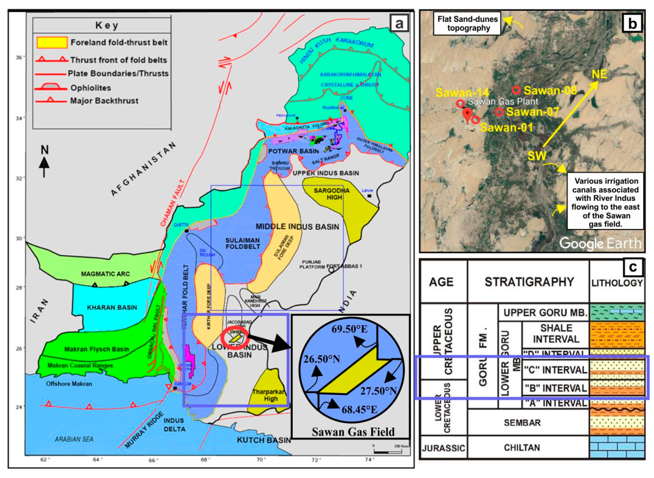
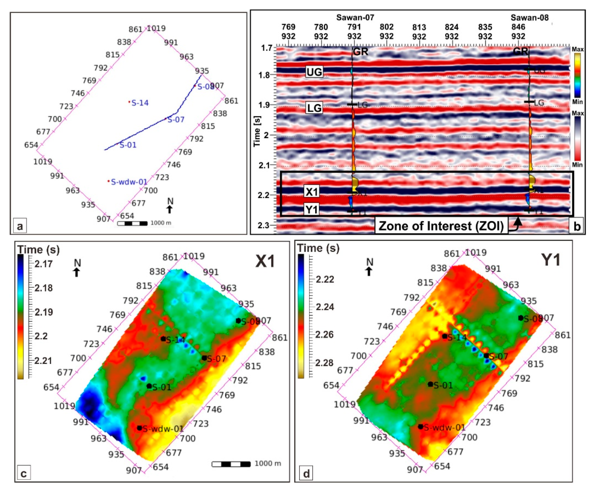
2. Stratigraphic and Structural Characteristics of the Study Area

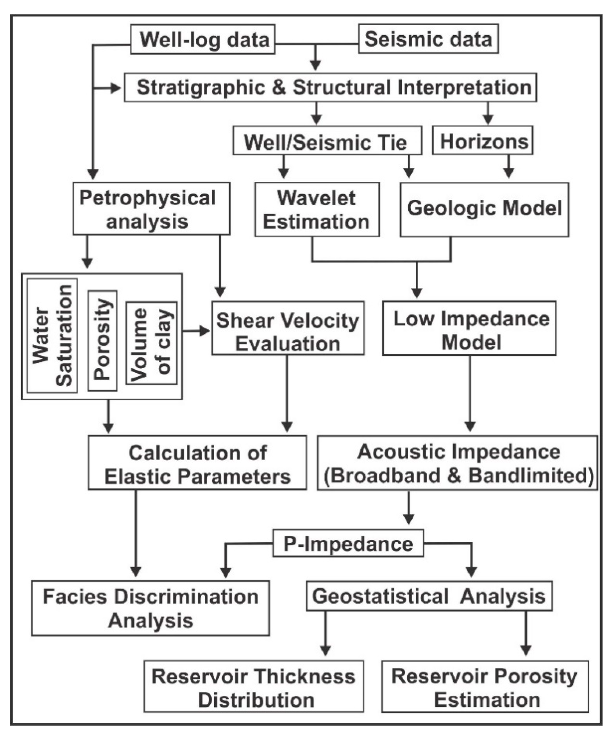
The SGF is located at the edge of the Middle Indus Basin (MIB) and Lower Indus Basin (LIB), having a maximum anticipated recovery of greater than one trillion cubic feet (TCF) and verified hydrocarbon reserved of three TCF. Henceforth, the study area is considered as one of the largest gas fields of the world and holds significant importance across all gas producing fields of Pakistan [34]. The study area abuts Jacobabad-Khairpur High (JKH) in the South, Indian Shield in East, Sulaiman Fold, Thrust Belt, and Kirthar Ranges in the West, while Sargodha-High in the North (Figure 1a) [36]. The wells of the SGF is situated in sand dunes topography, cut by different irrigation canals linked with the River Indus (Figure 1b). The discovery of SGF took place in 1997 and started yielding the production in 2003, and as of today, 14 wells are giving production [31].

The Precambrian basement and majority of the Cretaceous rocks within the LIB of the study area are tectonically stable [37]. The Precambrian basement is trigger by many lows and highs, which are the cause of significant lateral and vertical thickness variants of overlying sedimentary cover [38,39]. JKH demonstrated as horst is situated in the SGF amongst these highs and lows [40]. The Paleocene Ranikot clastics consist of detrital and carbonaceous sediments [41] pinches-out along the Khairpur-High that initiated the uplifting process. The JKH distributes the Indus Basin into the middle and lower parts and is considered as the main reason for the formation of structural traps within the SGF [42,43]. The Ranikot formation of the Paleocene pinched-out along JKH and caused the initial uplifting of the JKH. The structural and stratigraphic characteristics of the SGF are the cause of three tectonic episodes; late Cretaceous eroding and uplifting, NNW–SSE-directed basement rooted wrench faults and late Tertiary uplifting of JKH [44]. These NNW–SSE faults formed due to the transtension amid the collision of the Eurasian and Indian plates [45]. The orientation of the fault within the SGF is NNW–SSE oriented, while most of the fractures are characterized in the SE–NW direction [27].

The stratigraphy of the SGF includes the Jurassic age of the Chiltan limestone formation at the bottom that is covered by siliciclastic rocks of Cretaceous Sember and Goru formations to Quaternary alluvial rocks. The Goru Formation is further divided into LGF and Upper Goru Formation (UGF) [46]. The lower zone of the LGF is also distributed into D, C, B, and A-intervals (Figure 1c). The C-sand interval and B-sand interval of the Cretaceous age of the LGF acts as the primary and secondary reservoirs within the study area [32]. The principal lithologies of the LIB are shelf clastics and non-clastics, and marine-shales [47]. In contrast, the significant lithologies of the LGF are sand and shales. The reservoir sands were deposited in prograding proximal delta-front to delta distributaries in the shallow-marine environments [31,35].

Facies classification conducted through the well logging showed five lithofacies in the SGF representing deltaic fluvial-channel, delta-distributaries, and delta-front mouth-bars deposits as favorable environments for reservoir sands (Figure 2a,f). The mineralogy framework of the LGF is predominantly composed of the quartz (Q), chlorite (Chl), chlorite-rims (Chlr), volcanic rock fragments (VRF), and carbonates (mainly limestone). In contrast, the minor components of the LGF consist of feldspar grains (Fsp), glauconitic grains, and micas (Figure 2b,d). The secondary porosity within the reservoir sands occurred due to the dissolution of the feldspar grains. The chlorite exists as pore-lining cementing material, while calcite is observed in the form of a matrix, cement, fracture fillings, and carbonaceous material [48]. The presence of the fractures is the reason for the secondary porosity, whereas most fractures are E–W oriented and are clustered in the NW–SE directions [27]. The packing amid the Lower Goru sand (LGS) grains has sutured inter-granular and concave–convex contacts. The quartz overgrowth (Qo) exists together with the chlorite-rims (Chlr) (Figure 2c,e). In addition, the LGSs are mineralogically mature, and texturally sub-mature, moderate-to-poor sorted, angular-to-sub-angular in grain shapes, and coarse-to-very-fine in grain sizes. The 2D facies model of the LGF within the SGF shows an overall coarsening-upward trend. The model also highlighted that there are multiple lobes of the deltaic sediments, heading and prograding towards the low-energy mid-shelf marine settings. The reservoir sands of medium-to-coarse grains were deposited at the proximal delta-front region. In contrast, the non-reservoir fine-grained sediments (such as lime-mud, silt, and shale) were deposited at the distal pro-delta settings. The sediments of the LGF shows a lenticular shaped pattern, which is directed E–W and pinching-out in the NW direction. Cylindrical-shaped patterns mostly characterize the thick beds of gas-saturated reservoir sands. In contrast, non-reservoir quality sediments present at the bottom of the ZOI can be frequently observed as irregular-shaped trends (Figure 2a). These irregular patterns are acting as a seal in the petroleum play of the LGF in the SGF.

3. Data and Methods

The data were acquired from the Directorate General Concession Petroleum (DGPC), Ministry of Petroleum, Islamabad, Pakistan. The data attained in our study consist of 3D post-stacked seismic data that cover a vast area of the SGF. The well log data from five wells (S-01, S-07, S-08, S-14, and S-WDW-01) were used (Figure 3a). The S-WDW-01 is a water-disposable well. Numerous geophysical logs such as sonic (DT) (us/ft), density (RHOB) (g/cm³), neutron porosity (NPHI) (v/v), gamma-ray (GR) (API), spontaneous potential (SP) (m/V), deep resistivity (LLD) (ohm.m), shallow resistivity (LLS) (ohm.m), and micro-spherically focused resistivity (MSFL) (ohm.m) logs were incorporated to accomplish the aim of the research. The Jason software suite (InverTracePlus^TM module version 8.3) was utilized to accomplish the CSSI on the Sawan 3D cube.

Initially, seismic sections and well logs were analyzed to perform the stratigraphic and structural interpretation. A synthetic seismogram was established using the seismic-to-well tie method [49]. Based on robust reflection continuity, four horizons were marked within the Cretaceous Goru Formation named as Upper Goru Formation (UGF) and Lower Goru Formation (LGF) (Figure 3b). Within LGF, two targeted horizons X1 and Y1, were marked. The smoothing process was applied, and the interpolation of the geological model was run along the X1 and Y1 horizons to reduce the troughs and peaks. Two horizons X1 (C-sand interval) (Figure 3c) and Y1 (B-sand interval) (Figure 3d) within the targeted LGF were marked to interpret the extent of reservoir facies, reservoir thickness, and porosity distribution.

Secondly, the petrophysical analysis was conducted via geophysical logs using the stratigraphic correlation to calculate the thickness of the zone of interest (ZOI) via different wells. The petrophysical parameters were estimated using the structural correlation.

In the third step, RHOB and DT logs were incorporated to create the omitted p-impedance log. A wavelet was generated for each well to get the average wavelet. Extracted average wavelet, seismic, log data, and horizons were used simultaneously to make a low-frequency model that was combined with a bandlimited model to enhance the resolution of the inverted broadband model. Afterward, various quality control (QC) tests were performed to validate the inversion outcomes.

The geostatistical analysis was performed to analyze the impedance maps, porosity maps, and thickness maps to evaluate the sweet-spots and facies distribution. Facies discrimination analysis was conducted via rock physics modeling to distinguish the reservoir heterogeneity of sand-shale facies. In the last, factors controlling the reservoir heterogeneity were addressed. The complete workflow of the adopted methodology is shown in Figure 4.

A brief overview of the steps incorporated in executing our study are mentioned as follows.

4. Results

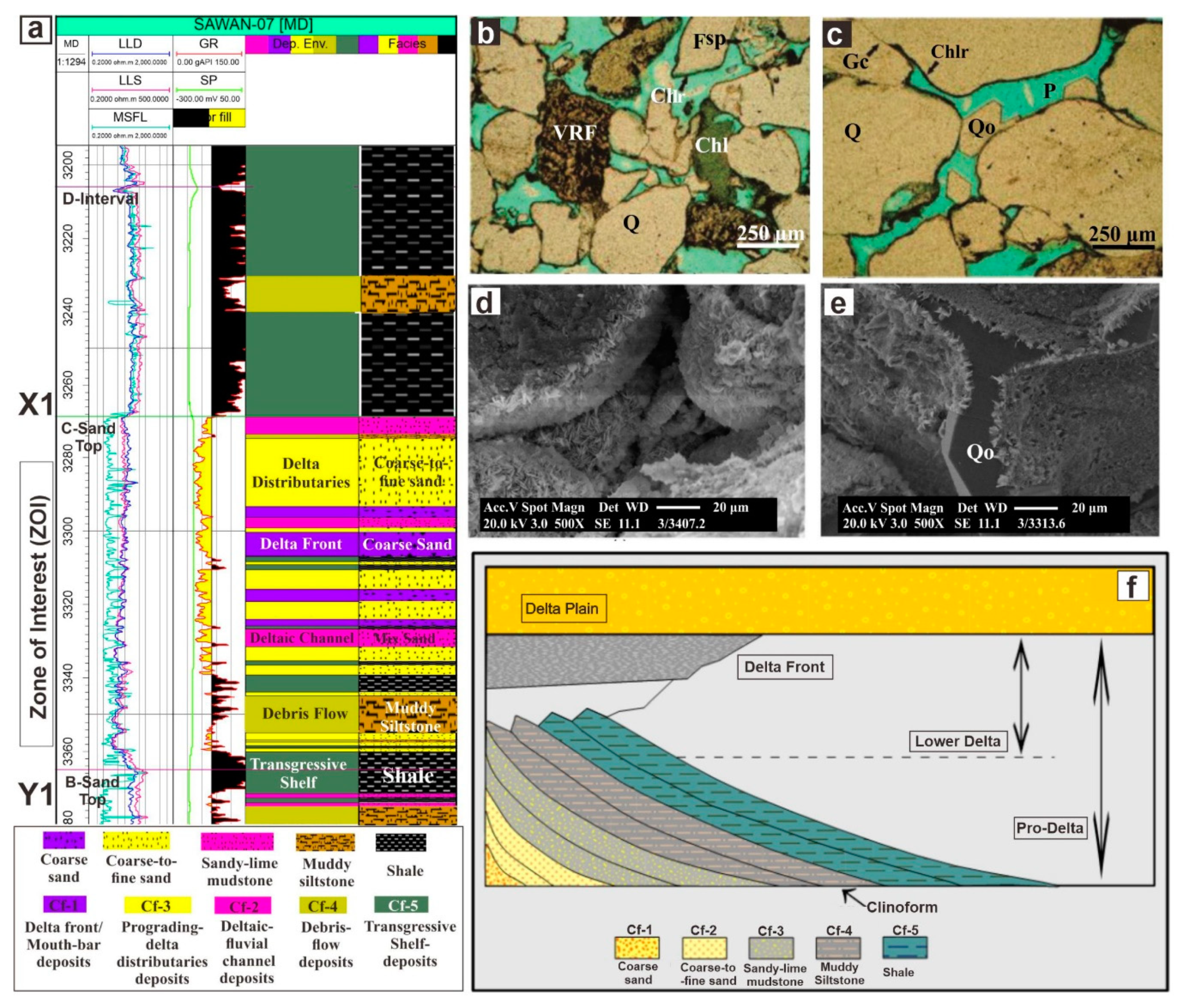
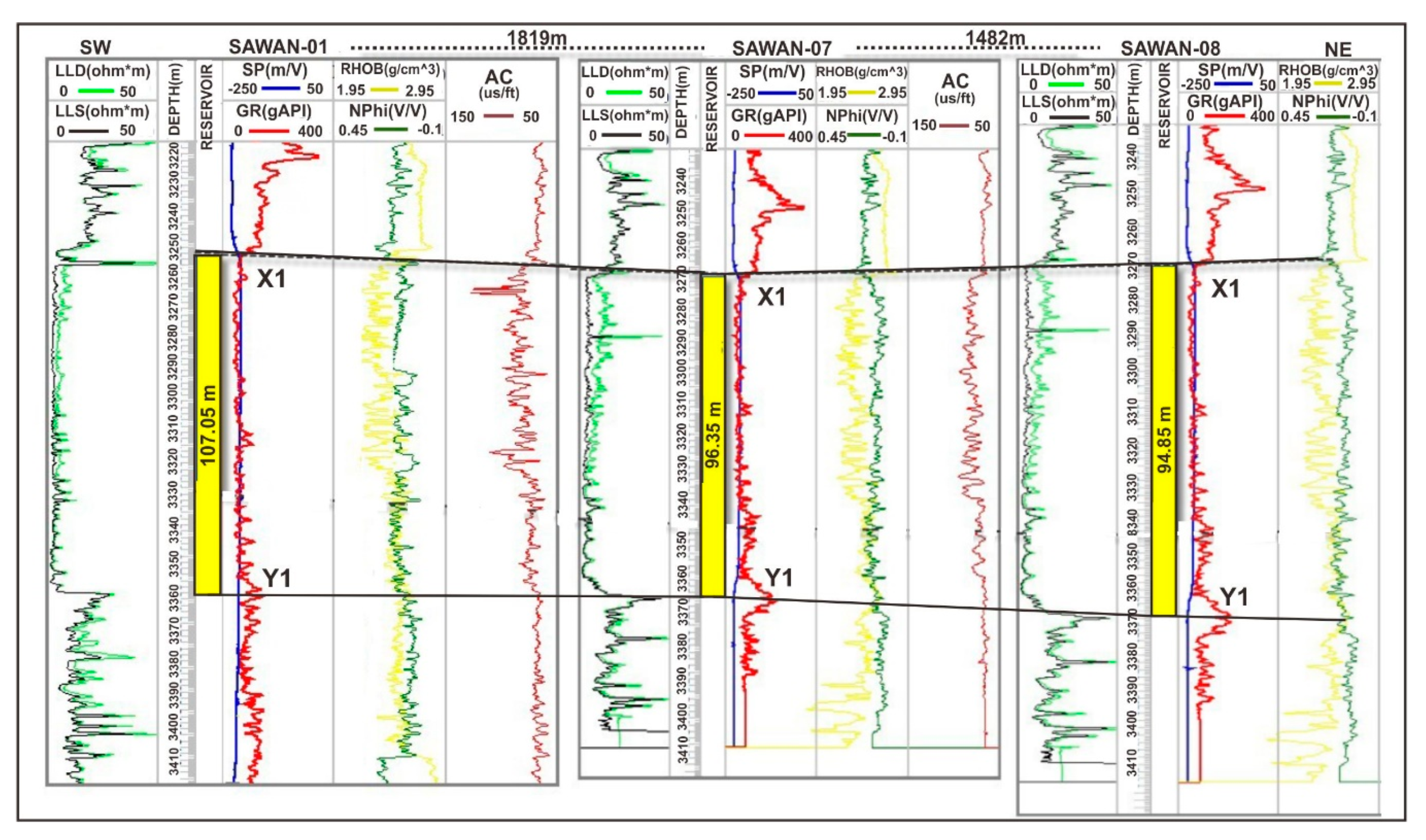
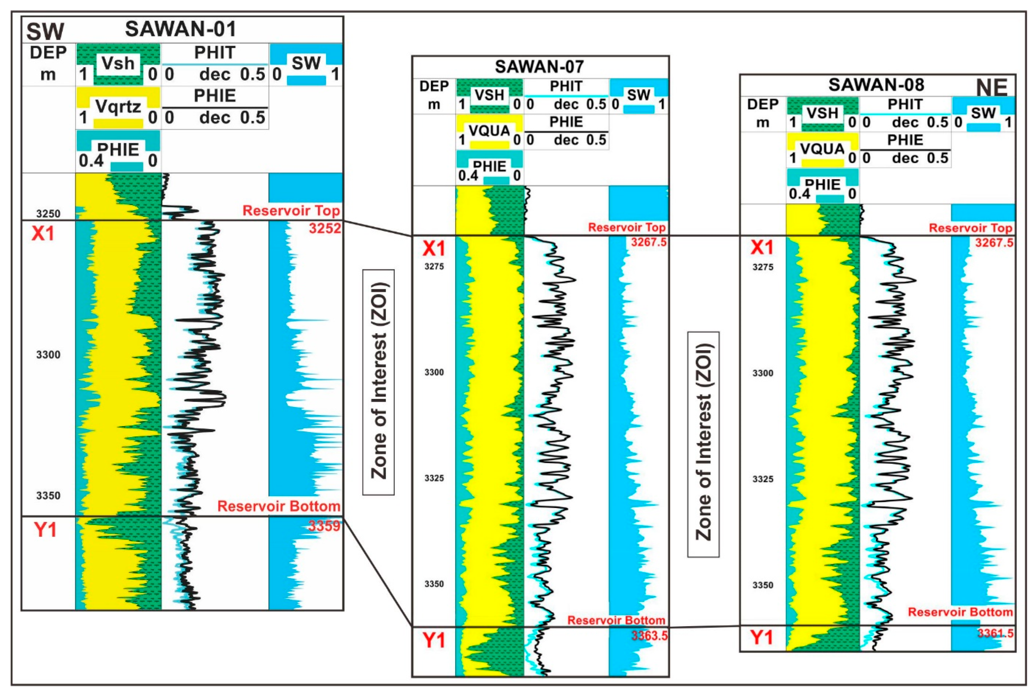
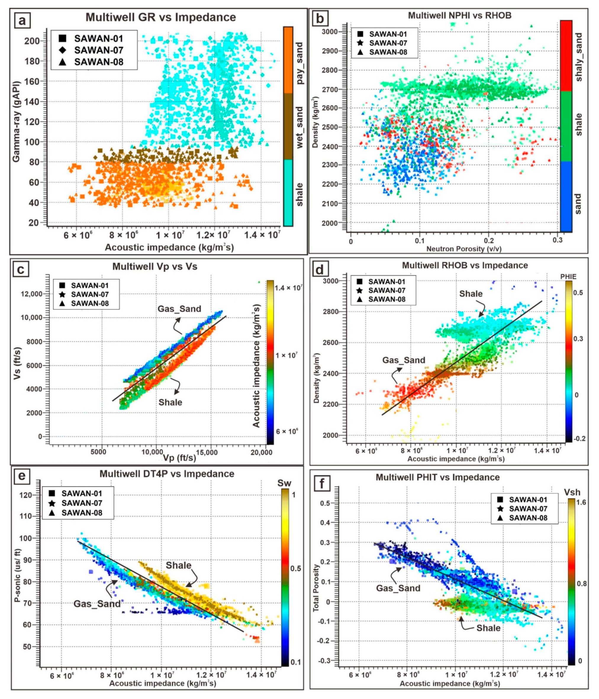
4.1. Petrophysical Analysis

The outcomes of the petrophysical study show that the narrow gap amid resistivity logs, crossover among RHOB and NPHI, high DT, and relatively low values of GR and SP highlights the ZOI that consists of thick porous and permeable sands. The thicknesses of ZOI in each well were different. The stratigraphic interpretation shows that the thickness of the reservoir C-sand interval differs from 107 m in the SW-oriented S-01 well to about 94 m in the NE-oriented S-08 well. Moreover, the thicknesses of the gas-saturated sands (pay-sands) ranges from 82.3 m to about 67.2 m (Figure 5). Since all the logs were not available in S-14, it was not incorporated in the analysis. Above and below the ZOI, there are high values of LLD (ohm.m), LLS (ohm.m), GR (API), SP (m/V), RHOB (g/cm³), and NPHI logs (v/v), which indicates the intermixing amid shale and sand layers.

The elastic logs were utilized to determine the structural configuration of the petrophysical parameters. The log conditioning was done before determining the reservoir parameters because it plays an essential role in improving the quality of the elastic logs. The increase in the quality of the logs ultimately increases the quality of the results. The reservoir properties such as the volume of quartz (V_qrtz), the volume of shale (V_sh), water saturation (S_w), and porosity were evaluated using the RHOB, NPHI, GR, and LLD logs. The V_sh was computed using the cross-plot analysis of neutron/density because the reservoir sands within the LGF of the SGF has high GR values [29,31] due to the presence of K-feldspar, chlorite, clay, glauconite, and mica [48]. The results of the structural correlation show that the ZOI consists of maximum porosity and V_qrtz (Figure 6).

In contrast, minimum V_sh and S_w within the ZOI highlight the region of thick porous and permeable gas-sands. However, high values of V_sh and S_w at the top and bottom of the ZOI highlights the presence of shale layers that are acting as a seal within the LGF. In the middle of the ZOI, there are relatively medium to high values of V_sh and S_w, and low values of porosity and V_qrtz suggests the presence of lime-mud and silt layers. The corollary, overall petrophysical analysis shows that the ZOI has good reservoir potential, and the thickness of the reservoir sands are thinning towards NE.

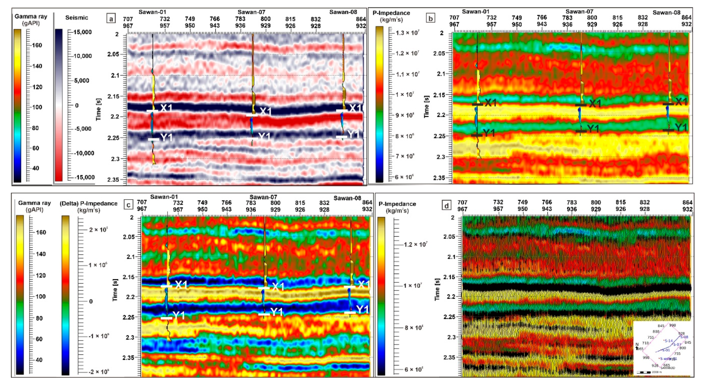
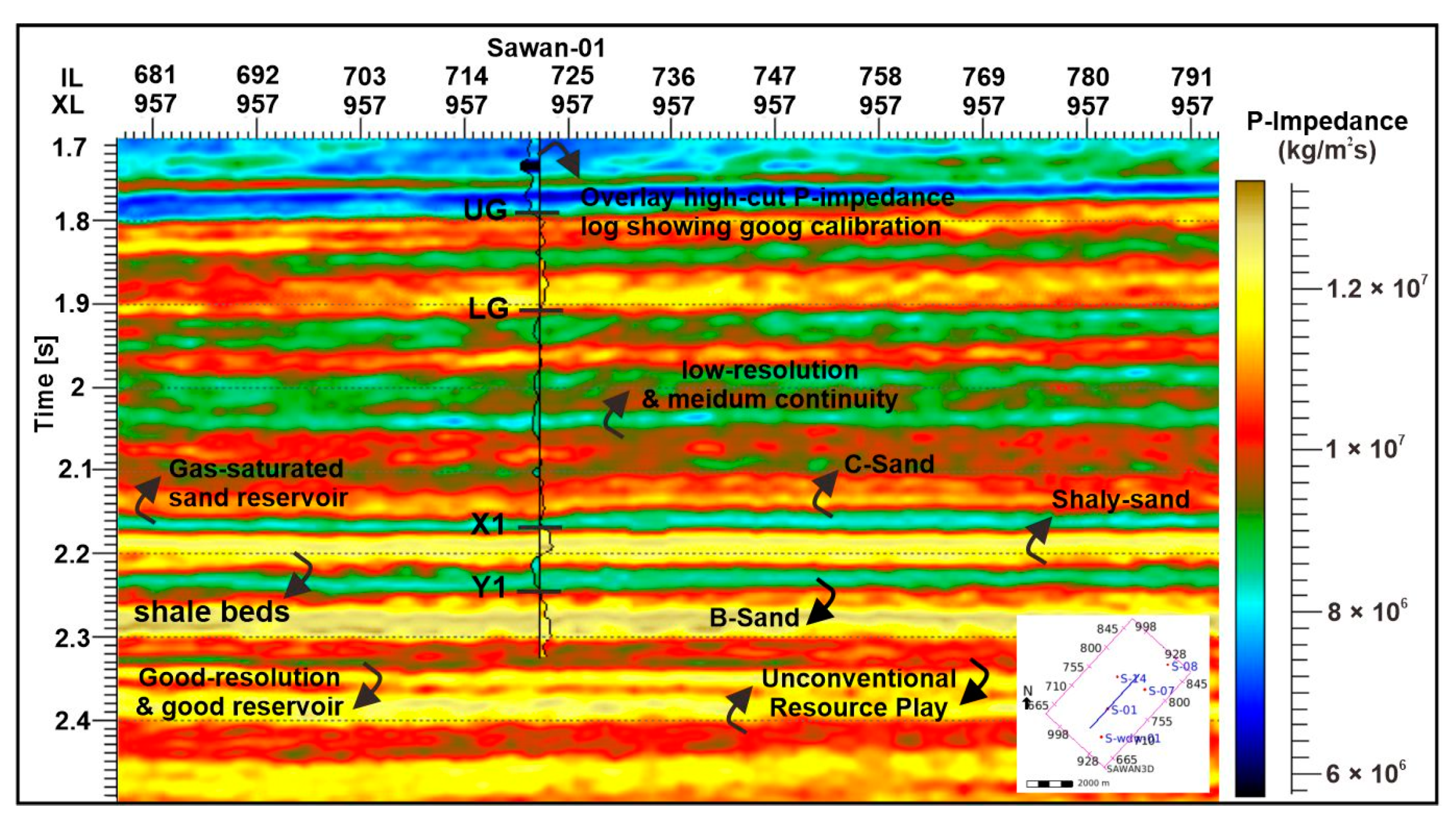
4.2. Inversion Analysis

4.2.1. Creating Missing Logs

Initially, the p-impedance log was not available in all study wells. The p-impedance log was created using the RHOB and p-sonic logs to generate the low-frequency AI model. Time-depth (T-D) conversion was performed by Backus’ averaging of the sonic log over the targeted time window. The data of all study wells were reviewed and edited, and the available data range for ZOI is selected from each well. Moreover, the density log was missing in S-14. The opted commercial software has a built-in algorithm that used Gardner’s method to create the missing density log [50].

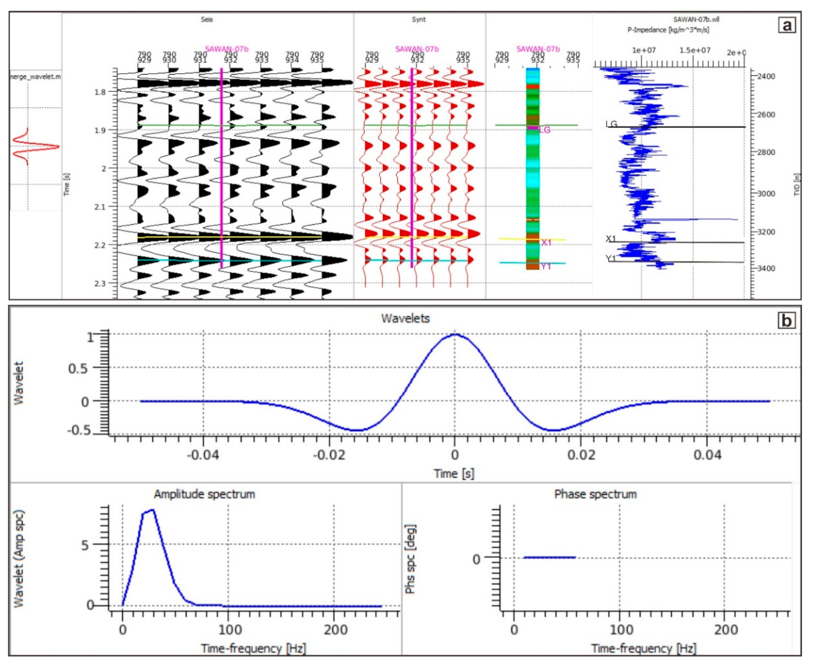
4.2.2. Wavelet Estimation

Accurate wavelet estimation is obligatory for attaining the dependable seismic inversion. A wavelet is associated with its amplitude spectrum and phase spectrum. As mentioned above, seismic and well data were tied using the synthetic seismogram, which was the essential first step for the process of wavelet estimation. The estimated wavelet was used to create synthetic seismograms, followed by the usual stretch and squeeze process using time-depth (T-D) functions to match the synthetics with the seismic data (Figure 7a). The process of the synthetic seismogram step is followed by an iterative method for the tying technique to improve the quality of the tie for the estimated wavelet until a suitable tie was reached.

The amplitude spectrum was calculated via auto-correlation, and the phase of the seismic data was removed through auto-correlation. The spectrum was smoothed using a time-taper to the auto-correlation function. The parameters set for estimating the wavelet are shown in

Table 1. Selected parameters for optimum wavelet estimation.

Sample Interval	Phase Rotation	Ricker Wavelet Frequency (Hz)	Correlation Factor	Correlation Range	Scale Factor	No. of Traces	Trace Gate (Horizons)
0.002	180°	22	0.79	0.02	72,401.9	10	LG—Y1

.

After the tie process, the wavelets were generated, and the susceptibility of the inversion process was checked with the different extracted wavelets. The wavelet used in the research was extracted from LG to Y1 horizons that completely encased the reservoir. The average wavelet for the available consistent wavelets was extracted using all the wells. The extraction of the average wavelet was carried out based on well locations and quality within the seismic survey (Figure 7b).

4.2.3. Low-Frequency Model (Earth Model)

Relative AI (a relative layer property) and absolute AI (an absolute layer property) are the two terms that are associated with AI. The difference between these two terms lies in producing the low-frequency model. Relative AI is used for qualitative interpretations and does not involve the low-frequency model. In contrast, the absolute AI is used for both qualitative and quantitative interpretations and includes the low-frequency (0–15 Hz) model in the algorithm of inversion [51]. Information regarding the low-frequency in the inversion algorithm for CSSI is added discretely [52]. Low-frequency noises within the seismic data interrupt the low-frequency data, which disrupts the recorded seismic data. Henceforth, the low-frequency model is introduced that provides a zero-hertz component to transform the relative AI values to absolute AI values, which delivers improved detection and resolution of the reservoir parameters.

The low-frequency AI model used in the research was given by [53], which is based on the iterative forward modeling approach [54]. In this model, integrated well-log data (mainly DT and RHOB logs), estimated seismic wavelet, 3D seismic data (bandlimited), and seismic horizons were used to mend the low-frequency information.

Since the AI inversion is bandlimited, a low-frequency model of AI was obligatory to produce the broadband AI model. This low-frequency model was extracted from interpolated well-log data and added to the band-limited AI model derived from seismic data. The triangulation interpolation method was used because it produced a continuous and smooth interpolation of data as compared to inverse distance weighted and kriging interpolation methods. The obtained low-impedance model gives a better insight to the lateral and vertical variation of the facies of the ZOI (Figure 8).

4.2.4. CSSI

The following steps were followed for checking the quality of the inversion process:

• The first step performed was to edit the trends. Usually, the value of the p-impedance increases with the depth, so the trends of all the wells using the targeted area (trace gate) was edited.
• Trace merging was done to merge a data set that provides the low-frequency band information with a data set that has the seismic bandwidth (or higher) information. The design (band-pass) filter was applied. The cutoff frequency was selected from 0 (lowest frequency) to 50 (highest frequency) Hz.
• Different QC parameters for the CSSI with lambda factor as a testing variable was performed.

After modifying all the QC parameters, CSSI was used to acquire the inverted bandlimited AI results. The addition of the low-frequency model to the developed AI model provides the necessary low-frequency missing information. All the various inversion products are used to get the best interpretation and full value from the inversion. The full bandwidth inversion results are the best for interpretation since they have the maximum bandwidth and minimum wavelet effects. Once areas and zones of interest have been identified on the uninterpreted seismic section (Figure 9a), the results were further analyzed using the full bandwidth result (Figure 9b). The bandlimited component was also examined to delineate the reservoir sandstone from the shales (Figure 9c). The dependability of the inverted AI absolute model was confirmed by analyzing the multiple tests.

Initially, an inverted AI absolute model was checked through by overlaying it on the seismic data (Figure 9d). The overlay showed that the inverted AI absolute model and the seismic data have the same resolution. Secondly, impedance sections can provide insight into geologic and simulation models. Therefore, overlay logs are used to confirm the reliability of the inverted model. As the vertical resolution of the seismic is less than the well logs, many beds seen in the wells are not visible in the seismic. To better compare the well logs with the inversion result, the well logs need to be high-cut filtered back to the frequency of the inversion result. Once filtered back, the p-impedance (Al) log and the GR logs were overlaid on the inverted seismic at different well locations, which confirms that the reservoir zone has minimum GR and minimum impedance values on the location of ZOI (Figure 9b,c and Figure 10).

These tests confirm that the inverted AI model is reliable and can be used for further reservoir characterization.

The CSSI method effectively delineated vertical and lateral variations in facies after integrating it with the low-frequency model. The anticipated ZOI lies from 2.1658 s (C-sand interval) to 2.213 s (B-sand interval) of LGF within the SGF. The range of the impedance lies form 8.58 × 10⁶ kg/m²s (C-sand interval) to 1.0357 × 10⁷ kg/m²s (B-sand interval) at S-07. These low-impedance values are suggesting the region of thick gas-saturated sand zone. These two intervals are separated with very high impedances (around 1.3 × 10⁷ kg/m²s), which shows that lime-mud and shale facies are present at the middle and bottom of the ZOI. The region above the ZOI (C-sand interval) also has a very high impedance (around 1.4 × 10⁷ kg/m²s) and high GR values (200 API), which indicates the presence of shale facies that belongs to the D-interval (which is acting as a seal in the study area). These results also support the petrophysical analysis results (Figure 5 and Figure 6), which confirm the reliability of the research work. Ref. [55] also suggested that low-impedance best describe the gas-saturated reservoirs, and the values of good gas reservoirs range from 8.0 × 10⁶ kg/m²s to 1.0 × 10⁷ kg/m²s. Henceforth, the reservoir sands in the ZOI of the SGF shows good agreement with the literature.

5. Discussion

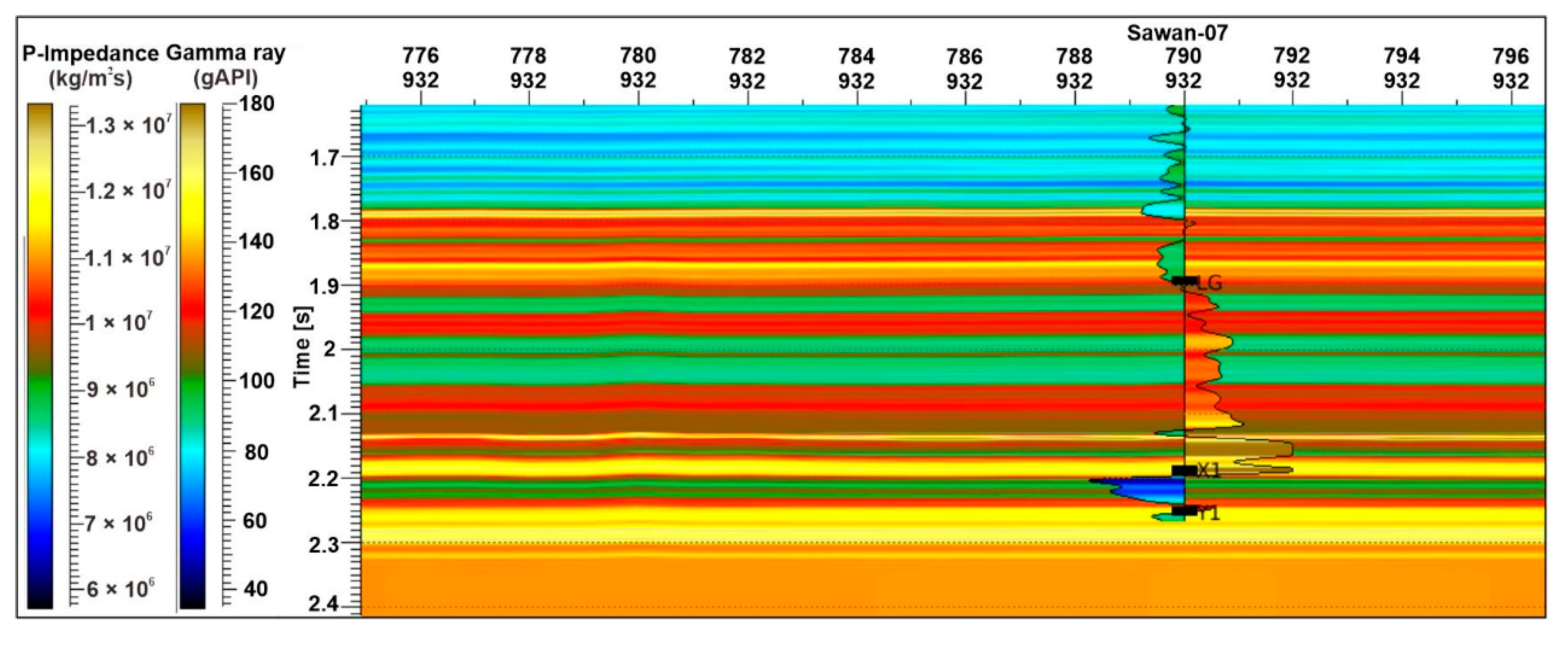
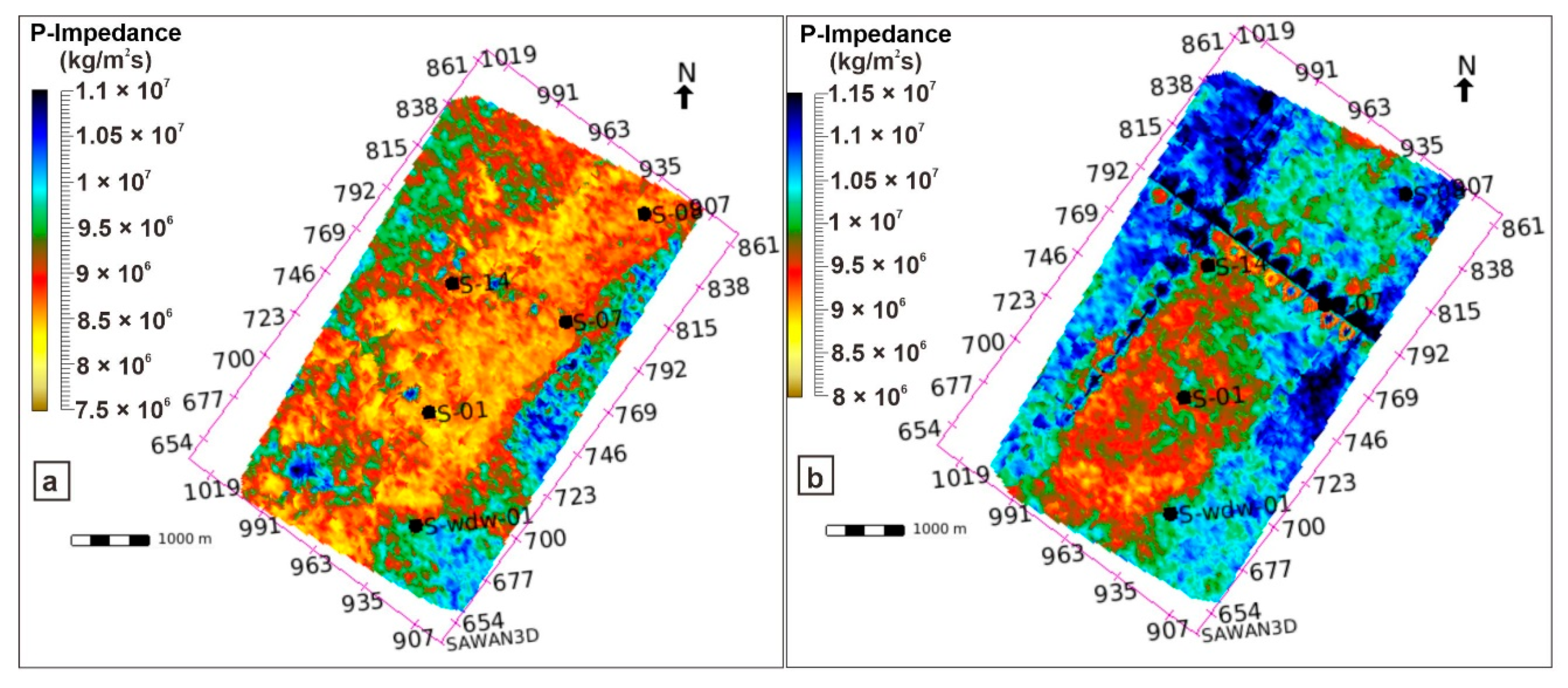
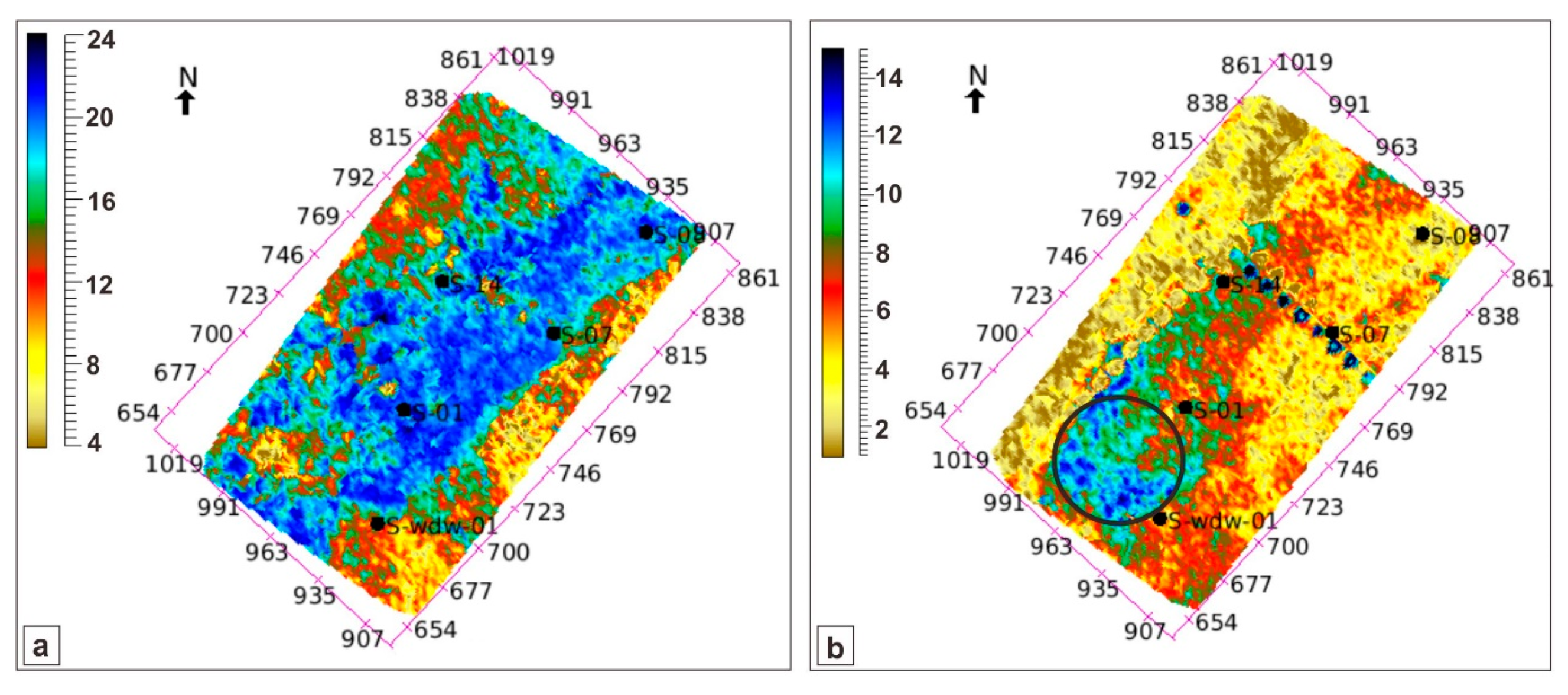
5.1. Distribution of the AI on the Targeted Sand Intervals

The AI maps within ZOI were generated to interpret the reservoir sand and shale facies distribution. A map of AI corresponding to the productive zone was extracted to compute the statistical attributes. The average root mean square (RMS) AI attribute was displayed since they give a superior image of the AI distribution. The results of the average RMS AI map of the C-sand interval shows that all the wells lie within the low-impedance zone (Figure 11a), which represents the gas-saturated sand facies. Whereas the impedance map of B-sand represents relatively low-impedance values at well locations (Figure 11b).

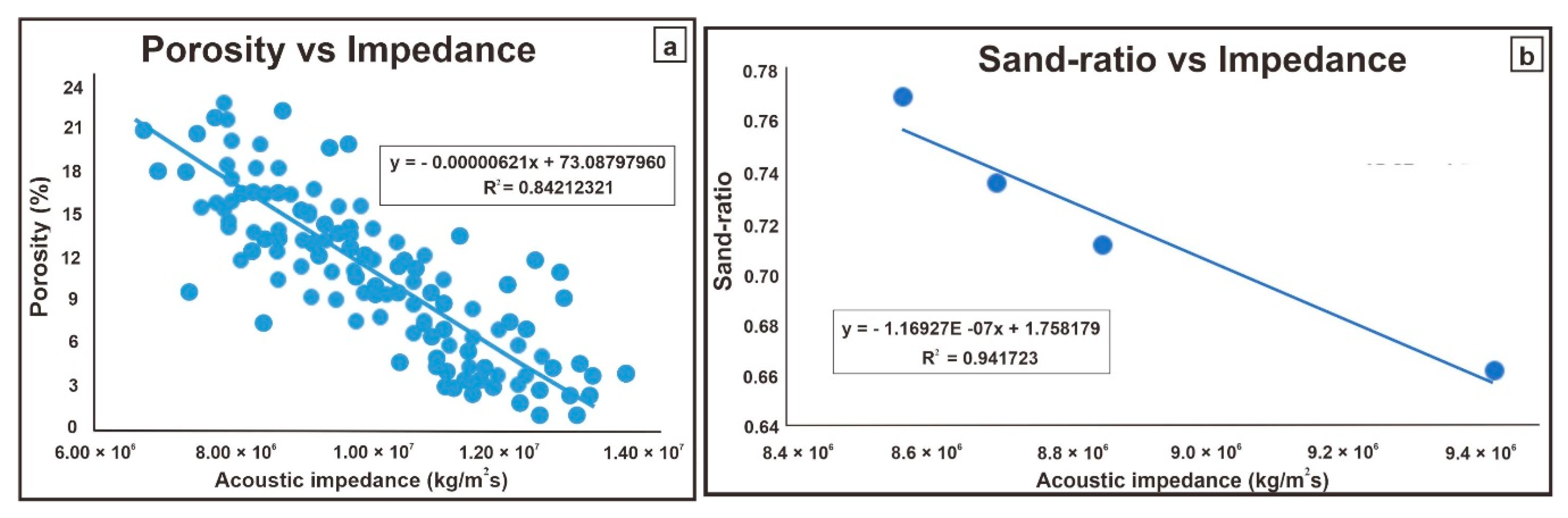
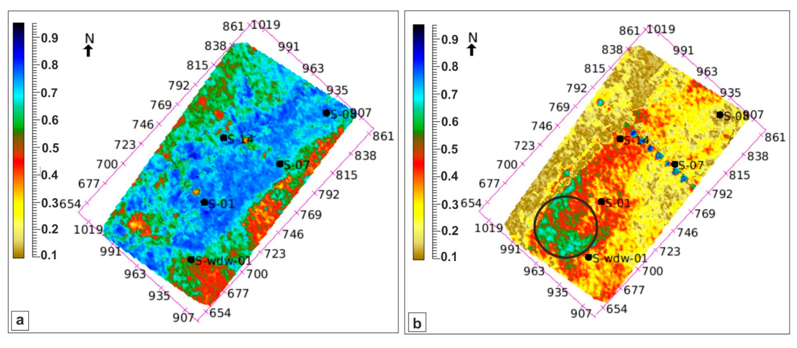
5.2. Reservoir Porosity Distribution by AI

To estimate porosities from the broadband AI volume, a relationship between them should be established. The well data were restricted to the ZOI for the estimation of porosities. Few points of high-GR values were observed in the ZOI because mudstone/limestone buildups of LGF pose some interbedded shales. These results can be correlated with lithologies and formations present in the study zone. Impermeable lithologies (high-GR) correspond to the presence of shale sediments within the reservoir zone, whereas the permeable lithologies (low-GR) correspond to sand sediments indicating the productive zone.

Once the well data was analyzed for the ZOI, a mathematical relation between the AI log and porosity log was determined. This relation was reached by cross-plotting the AI log and porosity log for all wells independently at ZOI. The relationships were achieved by computing a polynomial regression of second degree for each well to determine which well generates the best regression and trend. A linear regression technique was used to estimate the porosities because the AI and estimated porosities had a linear relationship. Since impedances and porosities are inversely proportional to each other, so the porosity increases with the decrease in the impedance, signifying a negative slope. The cross-plot amongst AI and porosity employing average values of all the wells at ZOI (from 3250 m to 3370 m) was prepared. The equation developed for the best-fit line amid AI and porosity has an inverse relationship (Figure 12a).

The corollary, the estimated porosities through the AI, is reasonable for the geological settings of the SGF. The acquired equation was used in the advanced calculations for making the statistics. The final porosity map shows reasonable matching with the results of impedance maps. All the study wells lie within a relatively good porosity zone. The porosity ranges from 12% to 24%, as shown in Figure 13a. The variation in the value of the porosities indicates variation in the lithology, which shows that lime-mud and silt have relatively low-porosity. The presence of thin shale layers among thick layers of sands represent a low value of porosity. High values of porosity among ZOI shows that the sands are porous and are highly productive.

Moreover, the C-sand interval represents a high value of porosity as compared to the B-sand interval. The B-sand interval is not the primary reservoir but shows decent porosity values. The SW region of B-sand (indicated by a black circle) shows high values of porosity maps that can be exploited for future drillings (Figure 13b). In addition, the S-08 and S-14 wells show high impedance values that can be attributed to the structural relief of the study area, which corresponds to the presence of fine-grained sand, silt, and shale facies. In addition, the S-01 and S-07 show low impedance values and hold a good reservoir potential with maximum sand thickness and maximum porosity S-01 and S-07 wells are attributed to the delta-front mouth-bars deposits where coarse-grained sands were deposited.

5.3. Reservoir Sand-Ratio Distribution by AI

Initially, interpreted lithology and depth column for the reservoir interval were exported from the well logging data. The top and bottom depths of each lithology were noted, and the thickness of each lithology was calculated. Then thicknesses of the sandstone intervals were added to get the total sand thickness. The total thickness of the formation interval was also calculated. The sand-ratio was evaluated using the formula:

Sand-ratio = sandstone thickness/formation thickness

The p-impedance value was noted from the inverted AI section at the corresponding well locations, and the steps were repeated for all four study wells (S-01, S-07, S-08, and S-14). The values of p-impedance and sand-ratio were plotted to get the linear relationship (trend-line), and an equation was obtained (Figure 12b). The equation derived from the trend-line was used for making the framework (statistics) using the inverted AI model. The final result obtained was displayed on the map, which supports the porosity and impedance map results. The sand-ratio thicknesses of S-01, S-07, S-08, and S-14 were 0.769, 0.735, 0.710, and 0.671. These values were calculated from the total sandstone thickness divided by the total formation thickness. Sand-ratio thicknesses at well-locations are higher for the C-sand interval as compare to the B-sand interval (Figure 14a). The southwest region of B-sand (shown by a black circle) shows high values of sand-ratio that can be exploited for future drillings (Figure 14b). In addition, the results of the sand-ratio show that the LGS are thinning from S-01 well towards S-08 well. The S-01 well has a maximum reservoir thickness.

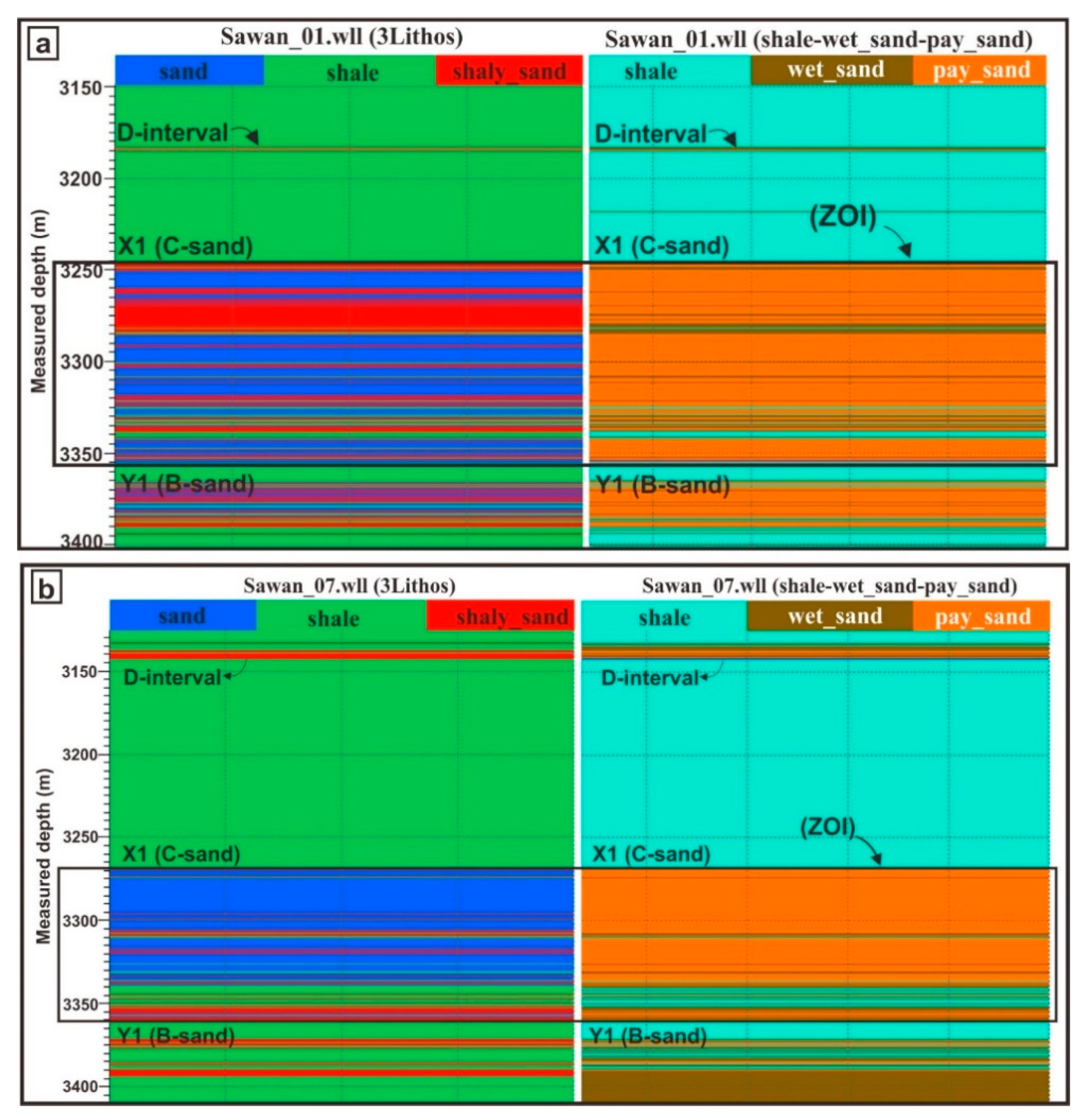
5.4. Distinction of Lithofacies by AI and Facies Logs

Facies were discriminated based on various petrophysical logs. Initially, the facies log was created using the GR log to distinguish the sand and shale facies using the if-then-else expression. A new user-defined lithofacies log named “3Lithos” was created with lithology types as sand, shale, and shaly_sand. The data were reduced to ZOI.

Afterward, another facies log was generated using the functions of GR and LLD log variables to discriminate the fluids such as pay-sands from the wet-sands using the if-then-else expression. Since the LLD log was missing in the S-14 well, it was skipped. Another user-defined lithofacies log named “shale-wet_sand-pay_sand” was created with lithology types as shale, wet_sand, and pay_sand (Figure 15a,b). The results of the created facies logs suggested that D-interval consists of thick beds of shale facies that lies above the ZOI. The average range of the pay-sand facies within the ZOI lies from 3256 m to 3361 m. The accumulation of pay-sands within the S-01 is relatively more significant than S-07. The lithofacies for S-07 and S-08 wells almost highlights the same behavior.

Duo quantitative and qualitative analysis was conducted to interpret the sand-shale heterogeneity using resistivity (LLD), gamma-ray (GR), density (RHOB), neutron porosity (NPHI), compressional velocity (V_p), shear velocity (V_s), the volume of shale (V_sh), water saturation (S_w), P-sonic, total porosity (PHIT), and effective porosity (PHIE) logs. The quantitative analysis was inspected to scrutinize the probability of sand and shale facies classification using the AI log. The extracted facies logs were also employed in the cross-plot study for facies discrimination using the AI log generated from the inversion analysis for S-01, S-07, and S-08 wells. The data were reduced to the targeted region. Initially, the facies were observed using the GR, and AI logs color-coded with extracted facies log (named shale-wet_sand-pay_sand) that distinguished the gas-saturated pay-sand facies with wet-sand and shale facies (Figure 16a). The relatively low values of GR and AI are associated with shallow-marine gas-saturated sand facies (pay-sand) that were deposited in the proximal delta-front settings. In contrast, the clustering of thin-laminations of shaly_sand (wet-sand) and shale facies suggest the intermixing of fine-grained facies that were deposited in the basinward marine depositional environment.

The RHOB-NPHI cross-plot color-coded with extracted facies log (named as 3Lithos) was used to differentiate the sand-shale facies. The relatively low values of RHOB and NPHI shows the sand facies, whereas the high values of RHOB and NPHI highlights the intermixing of shaly_sand and shale facies (Figure 16b).

The qualitative analysis for facies discrimination was investigated through cross-correlation amongst numerous logs. The direct or inverse relationship amid various logs helped us to identify and discriminate the lithofacies. The facies discrimination using only the compressional velocity (V_p) is not adequate enough due to the overlapping velocities of the reservoir. The shear velocity (V_s) was missing from the S-01 and S-07 wells. To understand the lithofacies composition of the reservoir, information was added to the V_p to understand the sand and shale heterogeneity. The V_s-V_p cross-plot color-coded with AI log showed a direct relationship, which displays that relatively high values of V_s and V_p and low AI are corresponding to the gas-saturated sand facies. In contrast, the relatively low values of V_s, V_p, and high AI are showing the intermixing of shaly_sand and shale facies (Figure 16c).

The RHOB-AI cross-plot color-coded with effective porosity (PHIE) log showed the direct relationship between RHOB and AI. The low values of RHOB and AI highlights the sand facies that are associated with maximum effective porosity values. In comparison, the shale facies are corresponding to negligible effective porosity and high RHOB and AI values (Figure 16d).

The P-sonic versus AI cross-plot color-coded by water saturation (S_w) highlighted the inverse relationship between them. The relatively high P-sonic values, low S_w, and AI values relate to the sand facies. In contrast, low P-sonic, high S_w, and high AI values are associated with shale facies (Figure 16e).

The PHIT-AI cross-plot color-coded with the volume of shale (V_sh) suggested an inverse relationship among them. The high total porosity, low AI, and V_sh show high porous gas-saturated sand facies. In addition, the high V_sh, low PHIT, and high AI values correspond to the shale facies (Figure 16f).

The cross-plot successfully predicted the probable lithofacies properties, highlighting a significant correlation to the AI to quantify lithology. Henceforth, the resulted sand-shale facies discrimination via AI inversion analysis can be further correlated to comprehend the lateral and vertical variations of facies to minimize the drilling risk for the LGF in the SGF. Consequently, transforming the resulted AI cube to facies volume would considerably expand our interpretation competency to demarcate heterogeneous reservoirs.

5.5. Reservoir Heterogeneity

A noteworthy difference in the thicknesses of the LGS was analyzed in the stratigraphic-cum-structural correlation via petrophysical analysis from SW to NE in the SGF (Figure 5 and Figure 6). In the LGF, the net reservoir thickness is thinning in the direction of a low-energy marine environment. This relationship is suggesting that the reservoir sands are prograding in the NE basinward direction [31]. The quality of the net-pay is deteriorating, and porosity in the LGS is decreasing in these NE thin sand-bodies. In contrast, the thickness is maximum towards the SW oriented S-01 well location. The presence of various depositional environments such as delta-front, delta-distributaries, fluvial-channels, and pro-delta deposits indicated the presence of very coarse to very fine sediments.

The results of the inversion analysis highlighted substantial vertical and lateral heterogeneity within the LGF. The deposition of the shallow-marine LGF is feasibly related to the presence of the narrower basement-rooted NNW–SSE wrench faults [32,33]. Hence, various shaly-sand and shale facies were conserved in the reservoir sands. Shale dispersal analysis performed by [56] suggested that the LGSs are categorized as vertically transversely isotropic (VTI) medium and composed of dispersed and laminated shale types. In addition, the authors predicted that these laminated shales contain thin beds of clays and do not control PHIE, S_w, and permeability of the rock. The high AI values within the ZOI is effectively highlighting these low-porosity pro-delta shaly-sand and transgressive shelf shale facies. In contrast, the middle and upper portion of the ZOI shows improved quality of the reservoir sands with substantial porosity of about 24%.

The LGS displays maximum temperature and pressure (around 170 °C and 37 MPa) because of a high geothermal gradient, overburden strata, and burial depth [29]. Due to these factors, the developed radiogenic heat becomes maximum, due to which the value of the GR within the LGS is relatively high (80 API). Henceforth, high geothermal gradient, high-temperature, maximum burial depth, overburden strata, growth of wrench faults, presence of coarse-to-fine sediments are the primary reasons controlling the reservoir heterogeneity within the LGF of the SGF.

The presence of very low porosity (less than 5%) at the bottom of the ZOI can be exploited as unconventional resource play (Figure 10). Further studies with proper evaluation are required to address the unconventional potential. In addition, the stratigraphic traps can be explored based on the AI, porosity, and sand-ratio maps. The corollary, the LGS has the best quality of the reservoir within the LIB.

6. Conclusions

The current research integrates petrophysical, geostatistical analysis, and rock physics along with constrained sparse spike inversion by utilizing 3D seismic and well log data for estimating porosity, sand-ratio, lithofacies, and reservoir heterogeneity. CSSI successfully resolved the sand and shale facies heterogeneities through bandlimited and broadband seismic data. The B- and C-sand intervals show low-impedance values (≈8.5 × 10⁷ kg/m²s) that indicated the gas-saturated sand facies zone, which is attributed to delta-front and fluvial-channel deposits. The two intervals are separated by a high-impedance region (≈1.3 × 10⁷ kg/m²s) that are associated with lime-mud, silt, and shale facies and corresponds to pro-delta deposits. The relationship between porosity and AI resulted in a high-correlation (0.84), whereas the regression between sand-ratio and AI resulted in an excellent degree of matching (0.941). The porosity of C-sand lies between 20–24%, whereas it lies from 10–14% for B-sand. The C-sand shows the sand-ratio of 0.9, whereas the B-sand reservoir shows the sand-ratio thickness of 0.6. The geostatistical and petrophysical analysis highlighted the spatial reservoir heterogeneity as the sand-ratio and porosity decrease towards the NE of SGF. This suggests that the facies thickness, reservoir heterogeneity, and reservoir quality is lithology reliant. The inverse relationship amid AI versus porosity showed that AI is a vital facies distinguisher. AI proved beneficial for qualitative and quantitative analysis for lithofacies prediction significantly when constrained through dependable petrophysical and petroelastic parameters. The current study has also predicted a region of high-porosity and maximum sand-ratio on B-sand time slice inverted maps that can be exploited for future drillings if adequately evaluated. C-sand interval is a proven reservoir within the study area. In addition, the current study has revealed that the B-sand also holds good reservoir potential and needs proper attention so that the problem of low-production from the deployed fields within the LGF can be reduced. We also suggest using the elastic impedance inversion for future research to invert the AI, RHOB, and V_pV_s ratio, which will extract numerous petroelastic parameters that will be proved vital from stratigraphic and sedimentological perspective.

References

1. Morozov, I.B.; Ma, J. Accurate poststack acoustic-impedance inversion by well-log calibration. Geophysics 2009, 74, R59–R67. [Google Scholar] [CrossRef]
2. Ashraf, U.; Zhu, P.; Yasin, Q.; Anees, A.; Imraz, M.; Mangi, H.N.; Shakeel, S. Analysis of balkassar area using velocity modeling and interpolation to affirm seismic interpretation, upper indus basin. Geosciences 2016, 6, 78–91. [Google Scholar]
3. Davarpanah, A.; Mirshekari, B.; Behbahani, T.J.; Hemmati, M. Integrated production logging tools approach for convenient experimental individual layer permeability measurements in a multi-layered fractured reservoir. J. Pet. Explor. Prod. Technol. 2018, 8, 743–751. [Google Scholar] [CrossRef] [Green Version]
4. Davarpanah, A. Feasible analysis of reusing flowback produced water in the operational performances of oil reservoirs. Environ. Sci. Pollut. Res. 2018, 25, 35387–35395. [Google Scholar] [CrossRef] [PubMed]
5. Shahab, A.; Qi, S.; Zaheer, M.; Rashid, A.; Talib, M.A.; Ashraf, U. Hydrochemical characteristic and water quality assessment for drinking and agricultural purposes in district jacobabad, lower indus plain, Pakistan. Int. J. Agric. Biol. Eng. 2018, 11, 115–121. [Google Scholar] [CrossRef]
6. Riaz, M.S.; Bin, S.; Naeem, S.; Kai, W.; Xie, Z.; Gilani, S.M.M.; Ashraf, U. Over 100 years of faults interaction, stress accumulation, and creeping implications, on chaman fault system, Pakistan. Int. J. Earth Sci. 2019, 108, 1351–1359. [Google Scholar] [CrossRef]
7. Zhu, M.; Yu, L.; Zhang, X.; Davarpanah, A. Application of implicit pressure-explicit saturation method to predict filtrated mud saturation impact on the hydrocarbon reservoirs formation damage. Mathematics 2020, 8, 1057. [Google Scholar] [CrossRef]
8. Abbas, A.; Zhu, H.; Anees, A.; Ashraf, U.; Akhtar, N. Integrated seismic interpretation, 2d modeling along with petrophysical and seismic atribute analysis to decipher the hydrocarbon potential of missakeswal area, Pakistan. J. Geol. Geophys. 2019, 7, 2. [Google Scholar]
9. Anees, A.; Shi, W.; Ashraf, U.; Xu, Q. Channel identification using 3D seismic attributes and well logging in lower Shihezi formation of hangjinqi area, northern Ordos Basin, China. J. Appl. Geophys. 2019, 163, 139–150. [Google Scholar] [CrossRef]
10. Xu, Y.-Z.; Huang, W.C.; Chen, T.J.; Cui, R.F.; Chen, S.Z. An evaluation of deep thin coal seams and water-bearing/resisting layers in the quaternary system using seismic inversion. Min. Sci. Technol. 2009, 19, 161–165. [Google Scholar] [CrossRef]
11. Saussus, D.; Sams, M. Facies as the key to using seismic inversion for modelling reservoir properties. First Break 2012, 30, 45–52. [Google Scholar] [CrossRef]
12. Veeken, P.; Rauch-Davies, M.; Gallardo, R.M.; Vera, E.G.; Villasenor, R.V. Seismic inversion of the Fortuna National 3D survey (Tabaso, Mexico). First Break 2002, 20, 287–294. [Google Scholar]
13. Pendrel, J. Seismic inversion—A critical tool in reservoir characterization. Scand. Oil-Gas Mag. 2006, 5, 19–22. [Google Scholar]
14. Abbasi, S.S.; Liu, J.; Hameed, N.; Ehsan, M. A modified approach for elastic impedance inversion due to the variation in the value of Κ. Earth Sci. Res. J. 2018, 22, 205–213. [Google Scholar] [CrossRef]
15. Campbell, T.J.; Richards, F.B.; Silva, R.L.; Wach, G.; Eliuk, L. Interpretation of the Penobscot 3D seismic volume using constrained sparse spike inversion, Sable sub-Basin, offshore Nova Scotia. Mar. Pet. Geol. 2015, 68, 73–93. [Google Scholar] [CrossRef]
16. Avadhani, V.; Anandan, M.; Thattacherry, B.J.; Murthy, K.S.; Gariya, B.C.; Dwivedi, A.K. Acoustic impedance as a lithological and hydrocarbon indicator—A case study from Cauvery Basin. Lead. Edge 2006, 25, 854–858. [Google Scholar] [CrossRef]
17. Farfour, M.; Yoon, W.J.; Kim, J. Seismic attributes and acoustic impedance inversion in interpretation of complex hydrocarbon reservoirs. J. Appl. Geophys. 2015, 114, 68–80. [Google Scholar] [CrossRef]
18. Latimer, R.B.; Davidson, R.; van Riel, P. An interpreter’s guide to understanding and working with seismic-derived acoustic impedance data. Lead. Edge 2000, 19, 242–256. [Google Scholar] [CrossRef]
19. Riedel, M.; Bellefleur, G.; Lee, M. Inversion of seismic data for elastic parameters: A tool for gas-hydrate characterization. In Geophysical Characterization of Gas Hydrates; Society of Exploration Geophysicists: Tulsa, OK, USA, 2010; pp. 109–120. [Google Scholar]
20. Zhu, H. Application of multiple wells-constrained sparse pulse inversion technology in coalfield 3D seismic prospecting. Procedia Earth Planet. Sci. 2011, 3, 401–407. [Google Scholar] [CrossRef] [Green Version]
21. Oldenburg, D.; Scheuer, T.; Levy, S. Recovery of the acoustic impedance from reflection seismograms. Geophysics 1983, 48, 1318–1337. [Google Scholar] [CrossRef]
22. Wang, Q.-F.; Guo, K. Constrained sparse spike inversion applied in the reservoir prediction. Well Logging Technol. 2008, 32, 35–37. [Google Scholar]
23. Simm, R.; Bacon, M. Seismic Amplitude: An Interpreter’s Handbook; Cambridge University Press: Cambridge, UK, 2014. [Google Scholar]
24. Barclay, F.; Bruun, A.; Rasmussen, K.B.; Alfaro, J.C.; Cooke, A.; Cooke, D.; Salter, D.; Godfrey, R.; Lowden, D.; McHugo, S.; et al. Seismic inversion: Reading between the lines. Oilfield Rev. 2008, 20, 42–63. [Google Scholar]
25. Hampson, D.P.; Schuelke, J.S.; Quirein, J.A. Use of multiattribute transforms to predict log properties from seismic data. Geophysics 2001, 66, 220–236. [Google Scholar] [CrossRef]
26. Qiang, Z.; Yasin, Q.; Golsanami, N.; Du, Q. Prediction of reservoir quality from log-core and seismic inversion analysis with an artificial neural network: A case study from the sawan gas field, pakistan. Energies 2020, 13, 486. [Google Scholar] [CrossRef] [Green Version]
27. Ashraf, U.; Zhang, H.; Anees, A.; Nasir Mangi, H.; Ali, M.; Ullah, Z.; Zhang, X. Application of unconventional seismic attributes and unsupervised machine learning for the identification of fault and fracture network. Appl. Sci. 2020, 10, 3864. [Google Scholar] [CrossRef]
28. Azeem, T.; Yanchun, W.; Khalid, P.; Xueqing, L.; Yuan, F.; Lifang, C. An application of seismic attributes analysis for mapping of gas bearing sand zones in the sawan gas field, Pakistan. Acta Geod. Geophys. 2016, 51, 723–744. [Google Scholar] [CrossRef]
29. Azeem, T.; Chun, W.Y.; Khalid, P.; Qing, L.X.; Ehsan, M.I.; Munawar, M.J.; Wei, X. An integrated petrophysical and rock physics analysis to improve reservoir characterization of Cretaceous sand intervals in Middle Indus Basin, Pakistan. J. Geophys. Eng. 2017, 14, 212–225. [Google Scholar] [CrossRef]
30. Xin, W.; Tian, F.; Shan, X.; Zhou, Y.; Rong, H.; Yang, C. Application of geologically constrained machine learning method in characterizing paleokarst reservoirs of tarim basin, China. Water 2020, 12, 1765. [Google Scholar] [CrossRef]
31. Ashraf, U.; Zhu, P.; Yasin, Q.; Anees, A.; Imraz, M.; Mangi, H.N.; Shakeel, S. Classification of reservoir facies using well log and 3D seismic attributes for prospect evaluation and field development: A case study of Sawan gas field, Pakistan. J. Pet. Sci. Eng. 2019, 175, 338–351. [Google Scholar] [CrossRef]
32. Azeem, T.; Chun, W.Y.; Khalid, P.; Ehsan, M.I.; Rehman, F.; Naseem, A.A. Sweetness analysis of Lower Goru sandstone intervals of the Cretaceous age, Sawan gas field, Pakistan. Episodes 2018, 41, 235–247. [Google Scholar] [CrossRef]
33. Ali, A.; Alves, T.M.; Saad, F.A.; Ullah, M.; Toqeer, M.; Hussain, M. Resource potential of gas reservoirs in South Pakistan and adjacent Indian subcontinent revealed by post-stack inversion techniques. J. Nat. Gas Sci. Eng. 2018, 49, 41–55. [Google Scholar] [CrossRef] [Green Version]
34. Yasin, Q.; Sohail, G.M.; Ding, Y.; Ismail, A.; Du, Q. Estimation of petrophysical parameters from seismic inversion by combining particle swarm optimization and multilayer linear calculator. Nat. Resour. Res. 2020, 1–27. [Google Scholar] [CrossRef]
35. Ali, M.; Ma, H.; Pan, H.; Ashraf, U.; Jiang, R. Building a rock physics model for the formation evaluation of the Lower Goru sand reservoir of the Southern Indus Basin in Pakistan. J. Pet. Sci. Eng. 2020, 194, 107461. [Google Scholar] [CrossRef]
36. Afzal, J.; Kuffner, T.; Rahman, A.; Ibrahim, M. Seismic and well-log based sequence stratigraphy of the early cretaceous, lower goru “C” sand of the sawan gas field, middle indus platform, Pakistan. In Proceedings of the Society of Petroleum Engineers (SPE)/Pakistan Association of Petroleum Geoscientists (PAPG) Annual Technical Conference, Islamabad, Pakistan, 17–18 November 2009. [Google Scholar]
37. Seeber, L. Seismotectonics of Pakistan: A Review of Results from Network Data and Implications for the Central Himalaya; Geol. Bull. University of Peshawar: Peshawar, Pakistan, 1980; Volume 13, pp. 151–168. [Google Scholar]
38. Aziz, H.; Ehsan, M.; Ali, A.; Khan, H.K.; Khan, A. Hydrocarbon source rock evaluation and quantification of organic richness from correlation of well logs and geochemical data: A case study from the sembar formation, Southern Indus Basin, Pakistan. J. Nat. Gas Sci. Eng. 2020, 81, 103433. [Google Scholar] [CrossRef]
39. Ehsan, M.; Gu, H.; Akhtar, M.M.; Abbasi, S.S.; Ehsan, U. A geological study of reservoir formations and exploratory well depths statistical analysis in Sindh Province, Southern Lower Indus Basin, Pakistan. Kuwait J. Sci. 2018, 45, 84–93. [Google Scholar]
40. Ahmad, N.; Fink, P.; Sturrock, S.; Mahmood, T.; Ibrahim, M. Sequence stratigraphy as predictive tool in lower goru fairway, lower and middle Indus platform, Pakistan. In Proceedings of the PAPG ATC, Islamabad, Pakistan, 8–9 October 2004; pp. 85–104. [Google Scholar]
41. Mangi, H.N.; Detian, Y.; Hameed, N.; Ashraf, U.; Rajpar, R.H. Pore structure characteristics and fractal dimension analysis of low rank coal in the Lower Indus Basin, SE Pakistan. J. Nat. Gas Sci. Eng. 2020, 77, 103231. [Google Scholar] [CrossRef]
42. Ahmad, N.; Chaudhry, S. Kadanwari gas field, pakistan: A disappointment turns into an attractive development opportunity. Pet. Geosci. 2002, 8, 307–316. [Google Scholar] [CrossRef]
43. Ali, M.; Khan, M.J.; Ali, M.; Iftikhar, S. Petrophysical analysis of well logs for reservoir evaluation: A case study of “Kadanwari” gas field, middle Indus basin, Pakistan. Arab. J. Geosci. 2019, 12, 215. [Google Scholar] [CrossRef]
44. Kazmi, A.H. Active fault systems in Pakistan. In Geodyn. Pak; Farah, A., DeJong, K.A., Eds.; Geodynamics of Pakistan. Geol. Sur. Pak: Quetta, Pakistan, 1979; pp. 285–294. [Google Scholar]
45. Kazmi, A.H.; Jan, M.Q. Geology and Tectonics of Pakistan; Graphic Publishers: Karachi, Pakistan, 1997. [Google Scholar]
46. Ehsan, M.; Gu, H.; Ahmad, Z.; Akhtar, M.M.; Abbasi, S.S. A modified approach for volumetric evaluation of shaly sand formations from conventional well logs: A case study from the talhar shale, Pakistan. Arab. J. Sci. Eng. 2019, 44, 417–428. [Google Scholar] [CrossRef]
47. Quadri, V.; Shuaib, S. Geology and hydrocarbon prospects of Pakistan’s offshore Indus basin. Oil Gas J. 1987, 85, 65–67. [Google Scholar]
48. Berger, A.; Gier, S.; Krois, P. Porosity-preserving chlorite cements in shallow-marine volcaniclastic sandstones: Evidence from Cretaceous sandstones of the Sawan gas field, Pakistan. AAPG Bull. 2009, 93, 595–615. [Google Scholar] [CrossRef] [Green Version]
49. Anees, A.; Zhong, S.W.; Ashraf, U.; Abbas, A. Development of a computer program for zoeppritz energy partition equations and their various approximations to affirm presence of hydrocarbon in missakeswal area. Geosciences 2017, 7, 55–67. [Google Scholar]
50. Gardner, G.H.F.; Gardner, L.W.; Gregory, A.R. Formation velocity and density—the diagnostic basics for stratigraphic traps. Geophysics 1974, 39, 770–780. [Google Scholar] [CrossRef] [Green Version]
51. Cooke, D.; Cant, J. Model-based seismic inversion: Comparing deterministic and probabilistic approaches. CSEG Rec. 2010, 35, 29–39. [Google Scholar]
52. Cooke, D.; Schneider, W. Generalized linear inversion of reflection seismic data. Geophysics 1983, 48, 655–795. [Google Scholar] [CrossRef]
53. Ferguson, R.J.; Margrave, G.F. A simple algorithm for band-limited impedance inversion. CREWES Res. Rep. 1996, 8, 1–10. [Google Scholar]
54. Veeken, P.C.H.; Da Silva, M. Seismic inversion methods and some of their constraints. First Break 2004, 22. [Google Scholar] [CrossRef]
55. Ibrahim, M. Seismic inversion data, a tool for reservoir characterization/modeling, sawan gas field—A case study. In Proceedings of the Annual Technical Conference 2007, Pakistan Association of Petroleum Geoscientists, Islamabad, Pakistan, 27–28 March 2007. Abstract No. 90140.2007. [Google Scholar]
56. Anwer, H.M.; Alves, T.M.; Ali, A. Effects of sand-shale anisotropy on amplitude variation with angle (AVA) modelling: The Sawan gas field (Pakistan) as a key case-study for South Asia’s sedimentary basins. J. Asian Earth Sci. 2017, 147, 516–531. [Google Scholar] [CrossRef] [Green Version]
Figure 1. (a) Regional geological map of Pakistan. The Sawan gas field (SGF) is located close to the Jacobabad-Khairpur High (JKH) north of the Lower Indus Basin (LIB) (highlighted by a blue square) [27]. (b) Location of the SGF showing the study wells on the imagery. (c) Stratigraphic chart of LIB. The blue rectangle highlights the zone of interest (ZOI) (modified from [35]).
Water 12 02972 g001
Figure 2. (a) Well-log facies classification of the S-08 well representing the various gamma-ray (GR) shape patterns for the identification of five lithofacies along with their depositional environment within the ZOI. (b,c) Thin-sections, and (d,e) scanning electron microscopy (SEM) images of the Lower Goru sands (LGSs) are illustrating the diagenetic features, where Q = quartz, Qo = idiomorphic quartz outgrowths, Chl = chlorite, Chlr = chlorite-rims, Gc = grain-contact, P = porosity is 16% [48]. (f) 2D cross-section showing the reservoir facies model of the Lower Goru Formation (LGF) within the SGF [31].
Water 12 02972 g002
Figure 3. (a) Basemap of the study area. The arbitrary line is selected that is passing through S-01, S-07, and S-08 wells, which were used for inversion analysis. (b) Seismic-to-well-tie of S-07 and S-08 at crossline-932. The black rectangle highlights the targeted area. (c) Interpolation of the X1 (C-sand) horizon. (d) Interpolation of the Y1 (B-sand) horizon.
Water 12 02972 g003
Figure 4. Workflow adopted for the current study.
Water 12 02972 g004
Figure 5. Stratigraphic correlation of study wells showing the thicknesses of ZOI in the study area.
Water 12 02972 g005
Figure 6. The structural configuration of study wells highlighting the thicknesses of the reservoir parameters within the ZOI.
Water 12 02972 g006
Figure 7. (a) Seismic-to-well tie among synthetic and seismic traces of S-07. X1 and Y1 horizons show the ZOI. (b) Average wavelet extracted along with amplitude and phase spectrum for study wells.
Water 12 02972 g007
Figure 8. Earth model with GR overlay, which highlights the ZOI with blue filling representing low-GR values.
Water 12 02972 g008
Figure 9. Well-tops, overlay GR (API) log, and S-01, S-07, S-08 wells on (a) a seismic section. (b) Inverted AI broadband model. (c) Inverted AI broadband model with well-tops, overlay GR (API) log, and S-01, S-07, S-08 wells. (d) Overlay of seismic section (wiggle) and inverted broadband AI model that shows the same resolution.
Water 12 02972 g009
Figure 10. Overly of p-impedance log on inverted AI section at S-01 well and crossline-957 location.
Water 12 02972 g010
Figure 11. AI maps of (a) C-sand interval and (b) B-sand interval.
Water 12 02972 g011
Figure 12. Regression analysis of multi-well for (a) porosity and impedance. (b) Sand-ratio versus impedance.
Water 12 02972 g012
Figure 13. Porosity distribution maps of (a) C-sand interval and (b) B-sand interval. The black circle shows the high porosity region with no drilled well and can be exploited for future drillings.
Water 12 02972 g013
Figure 14. Sand-ratio distribution maps of (a) C-sand interval; (b) B-sand interval. The black circle shows the high sand-ratio region with no drilled well and can be exploited for future drilling.
Water 12 02972 g014
Figure 15. Facies log created for LGF using GR log to differentiate the sand (blue), shale (green), and the shaly_sand (red) facies (left side). Whereas, facies log generated using GR and resistivity (LLD) log to differentiate the pay-sands (orange), wet-sands (brown), and shale (cyan) facies (right side) for (a) S-01, and (b) S-07.
Water 12 02972 g015
Figure 16. Facies discrimination analysis using AI and facies logs cross-plots. (a) GR-AI cross-plot color-coded with generated shale-wet_sand-pay_sand facies log showing the cutoff values for gas-sand (pay-sands) and shaly-sand (wet-sands) and shale sediments. (b) Neutron-Density cross-plot color-coded with extracted 3Lithos facies log showcasing the sand and intermixing of shaly-sand and shale facies. The mixing of thin-laminated fine-grained shaly-sand and shale facies shows scattered plotting. (c) Vs-Vp cross-plot color-coded with AI log highlighting good separation of gas-sand and shale facies. (d) RHOB-AI cross-plot color-coded with effective porosity log displays reliable discrimination of porous gas-sand facies versus non-porous shale facies. (e) P-sonic-AI cross-plot color-coded with Sw distinguishing the clean sand and shale facies. (f) Total Porosity-AI cross-plot color-coded with Vsh highlights excellent discrimination of porous gas-saturated sand facies and non-porous shale facies.
Water 12 02972 g016