Improved Membrane Inlet Mass Spectrometer Method for Measuring Dissolved Methane Concentration and Methane Production Rate in a Large Shallow Lake

Abstract

Natural water bodies, such as lakes, rivers, and oceans, are important sources of atmospheric methane (CH₄). Therefore, quantitative and accurate determination of the dissolved CH₄ concentration in water is of great significance for studying CH₄ emissions and providing an in-depth understanding of the carbon cycle. Headspace gas chromatography (HGC) is the traditional method for measuring CH₄ in water. Despite its long success, it has a lot of problems in use, such as complex pretreatment and a long measurement time, and it is not suitable for the CH₄ determination of a large number of samples. In view of these shortcomings, a more convenient and efficient method based on membrane inlet mass spectrometry (MIMS) for quantitative measurements of the dissolved CH₄ concentration in water was established. In our study, the standard curves showed that the method had high accuracy, both at low and high CH₄ concentrations. After a laboratory test, to evaluate the sensitivity of this method, samples were collected from a large shallow lake (Lake Taihu). Both the HGC method and MIMS method were used to determine the dissolved CH₄ to compare these two methods. The small difference in CH₄ concentration obtained from the MIMS and HGC methods and the significant correlation between the CH₄ concentrations derived from the MIMS method with those derived from the HGC method showed that the MIMS method could replace the HGC method in the determination of dissolved CH₄ in natural waters. In addition, we also measured the sediment CH₄ production rates in three different areas of Lake Taihu using a laboratory incubation experiment. During the experiment, significant CH₄ accumulations were observed, indicating that sediment CH₄ production was an important source of dissolved CH₄ in the water column. Our study concluded that the MIMS method was sufficient and a better alternative than the HGC method owing to its capacity to measure a broad range of values plus the fact that it was relatively easy to use with less manipulation of the samples.

1. Introduction

Greenhouse gases mainly include methane (CH₄), carbon dioxide, and nitrous oxide, which can lead to the greenhouse effect, which is having a significant impact on the natural ecosystem, such as climate anomalies, melting glaciers, and increasing sea levels [1,2,3,4]. Although the CH₄ concentration in the atmosphere is very low compared with carbon dioxide, the greenhouse effect of CH₄ is more than 21–23 times that of carbon dioxide [5].

As important sources of CH₄, natural water bodies, such as lakes, oceans, and reservoirs, have attracted much attention [6,7]. Therefore, there is a great demand for determining the dissolved CH₄ concentrations in waters. Although the concentration of CH₄ in waters cannot be used to directly quantify the CH₄ emissions to the atmosphere, it can reveal the potential of CH₄ diffusion from waters to the atmosphere. In addition, the CH₄ diffusive flux can be calculated through Fick’s first law if we know the dissolved CH₄ concentration, corresponding water temperature, salinity, and wind speed [7,8], which indicates that if we can quickly and accurately determine the concentration of the dissolved CH₄, it seems to be simpler and more convenient to calculate the CH₄ diffusion from natural waters. Meanwhile, an accurate and effective method for the determination of dissolved CH₄ can help us to estimate the CH₄ production or oxidation capacity in waters, which is of great significance to the study of the fate of CH₄.

Traditionally, the main method for the determination of CH₄ in water is headspace gas chromatography (HGC), which requires complex pretreatment [9]. The HGC method is widely used in the determination of CH₄ and nitrous oxide in natural water bodies [10,11], but this method cannot directly measure the concentration of dissolved CH₄ in waters, resulting in low efficiency. Thus, a more convenient and efficient method is desired. Although CH₄ measurements using MIMS go back to the 1980s [12], this technique has not been generally used for environmental water sample measurements. As a relatively new method in environmental science for measuring dissolved gases in water, membrane inlet mass spectrometry (MIMS) has attracted much attention owing to its high precision, convenience, and efficiency. MIMS instruments can be configured with a variety of membrane interfaces, including probes, flat membranes in chambers, and flow-through tube membranes [13]. Using a tube membrane with a highly stable flow and temperature control results in highly stable signals with very high precision of gas ratios (better than 1 per mil). This form of MIMS has become the standard for measuring the N₂/Ar ratio and ¹⁵N in denitrification studies, which require very high precision measurements [14]. MIMS has had limited use for measuring CH₄ in environmental samples and the vast majority of aquatic CH₄ studies utilize alternative methods, such as gas chromatography (GC). Given the high precision and convenience of MIMS for measuring dissolved air gases using the standard methods for denitrification [15,16], we evaluated this analytical approach for CH₄ detection in lake water samples. A recent study used the MIMS method to measure the CH₄ concentration in culture experiments by using the ratio relative to Ar (CH₄:Ar ratio) [17]. However, this calculation method has a great problem in that the Ar determination using the MIMS method can be greatly affected by the O₂ concentration [18]. Here, we used the standard curve method to accurately calculate the dissolved CH₄ concentration based on the MIMS method.

With the considerations mentioned above, we tested the reliability of the MIMS method for measuring the CH₄ concentration in the laboratory. Furthermore, we also sampled water samples from a large shallow lake, namely, Lake Taihu, to verify that this method is also suitable for dissolved CH₄ concentration measurement in natural waters. Sediment cores were also collected from Lake Taihu to quantify the sediment CH₄ production rate to show that this method is appliable in culture experiments.

2. Materials and Methods

2.1. CH₄ Measurement Approach Using MIMS

MIMS uses a sampling probe or water sampler equipped with a gas-permeable membrane that separates the water sample from the vacuum of the mass spectrometer. The MIMS in this study (Bay Instruments) includes a tube membrane inside the vacuum inlet (Figure 1). Water samples are pumped through stainless steel tubing in a thermostated bath (20 °C) prior to entering the vacuum inlet where the membrane tube resides. The flux of dissolved gases across the membrane depends on the flow velocity and temperature and these parameters were held constant. All samples were measured at 20 °C. The gas stream was dried using a liquid nitrogen U-tube trap prior to entering the mass spectrometer. The instrument signals were assessed for stability by pumping temperature-controlled (±0.02 °C) water through the membrane [14].

2.1.1. Preparation of Standard Samples

CH₄ standard samples were prepared using a headspace equilibrium method. A pressurized container containing 99.99% CH₄, a sealed gas collecting bag, and a quantitative syringe were used to transfer CH₄ to 12 mL Labco Exetainer vials. Before the addition, the vial volume was calibrated by weighing the water of a filled vial. After calibration, 7 mL of deionized water was added, leaving a 5 mL headspace. A known amount of CH₄ was injected into the headspace through a quantitative gas-tight syringe. The vials were shaken for 5 min or more and then were put into a thermostatic water bath for solubility equilibration.

2.1.2. Measurement of Standard Samples

CH₄ was conventionally measured with MIMS using mass 15, which was the CH₃⁺ fragment of CH₄, avoiding the pronounced and variable mass 16 peak that is associated with O⁺. This fragment was 90% of the intensity of the mass 16 peak of CH₄ and sat on a low baseline peak. For nanomolar and low micromolar concentrations, it was necessary to use the secondary electron multiplier (SEM) detector.

2.1.3. Calculation of Dissolved CH₄ in Standard Samples

The concentration of dissolved CH₄ in standard samples was calculated according to Henry’s law and Dalton’s law. Henry’s law was put forward by William Henry in 1803. It was applicable to the situation that there was no chemical reaction in the system and the temperature was constant. In this case, Henry’s law states that the concentration of the gas dissolved in the liquid would be proportional to the partial pressure of the gas in the gaseous phase. Dalton’s law states that for a gas mixture without a chemical reaction, the total pressure is equal to the sum of the partial pressures of all gases in the mixture. The specific formulas were as follows:

$${\mathrm{C}}_{\mathrm{water}}^{{\mathrm{CH}}_4}={\mathrm{P}}_{{\mathrm{CH}}_4}\times \mathrm{H}$$

(1)

$$\mathrm{H}=\mathsf{\beta }/{\mathrm{V}}_{\mathrm{m}}$$

(2)

$$\ln (\mathsf{\beta })={\mathrm{A}}_1+{\mathrm{A}}_2\times 100/\mathrm{T}+{\mathrm{A}}_3\times \ln \left(\mathrm{T}/100\right)+\mathrm{S}\times \left[{\mathrm{B}}_1+{\mathrm{B}}_2\times \mathrm{T}/100+{\mathrm{B}}_3\times {\left(\mathrm{T}/100\right)}^2\right]$$

(3)

where H is the solubility coefficient of CH₄ (mol (L atm)⁻¹), ${\mathrm{C}}_{\mathrm{water}}^{{\mathrm{CH}}_4}$ is the CH₄ concentration in water (mol L⁻¹), ${\mathrm{P}}_{{\mathrm{CH}}_4}$ is the partial pressure of CH₄ in the headspace after reaching equilibrium. β is Benson’s solubility coefficient. A₁, A₂, A₃, B₁, B₂, and B₃ are constants and can be derived from previous studies [19]. S is the salinity of the solution (‰). T represents the water temperature (K). V_m is the molar volume.

$${\mathrm{P}}_{{\mathrm{CH}}_4}=\frac{{\mathrm{V}}_{\mathrm{HS}}^{{\mathrm{CH}}_4}}{{\mathrm{V}}_{\mathrm{HS}}}\times {\mathrm{P}}_{\mathrm{tot}}$$

(4)

$${\mathrm{P}}_{\mathrm{tot}}=\frac{{\mathrm{V}}_{\mathrm{inj}}^{{\mathrm{CH}}_4}+{\mathrm{V}}_{\mathrm{HS}}}{{\mathrm{V}}_{\mathrm{HS}}}\times \mathrm{P}$$

(5)

where ${\mathrm{V}}_{\mathrm{HS}}^{{\mathrm{CH}}_4}$ is the volume of CH₄ in the headspace after reaching equilibrium (L), VHS is the volume of headspace in the vial (L), P_tot is the total pressure in the vial, P is the standard atmospheric pressure at 20 °C, and ${\mathrm{V}}_{\mathrm{inj}}^{{\mathrm{CH}}_4}$ is the volume of the injection (L). Because the solubility of CH₄ is very low, changes in the total pressure due to the dissolution of CH₄ were ignored, indicating that the total pressure in the headspace was constant during the dissolution.

$${\mathrm{V}}_{\mathrm{HS}}^{{\mathrm{CH}}_4}+{\mathrm{V}}_{\mathrm{water}}^{{\mathrm{CH}}_4}={\mathrm{V}}_{\mathrm{inj}}^{{\mathrm{CH}}_4}+{\mathrm{V}}_{\mathrm{HS}}^{{\mathrm{CH}}_4^{*}}+{\mathrm{V}}_{\mathrm{water}}^{{\mathrm{CH}}_4^{*}}$$

(6)

$${\mathrm{V}}_{\mathrm{water}}^{{\mathrm{CH}}_4}={\mathrm{C}}_{\mathrm{water}}^{{\mathrm{CH}}_4}\times {\mathrm{V}}_{\mathrm{water}}\times {\mathrm{V}}_{\mathrm{m}}$$

(7)

where ${\mathrm{V}}_{\mathrm{HS}}^{{\mathrm{CH}}_4^{*}}$ is the volume of CH₄ in the headspace before injection (L), ${\mathrm{V}}_{\mathrm{water}}^{{\mathrm{CH}}_4^{*}}$ is the volume of CH₄ in the water before injection (L), ${\mathrm{V}}_{\mathrm{HS}}^{{\mathrm{CH}}_4^{*}}$ is measured using GC, and ${\mathrm{V}}_{\mathrm{water}}^{{\mathrm{CH}}_4^{*}}$ is measured according to Equation (8):

$${\mathrm{C}}_{\mathrm{water}}^{{\mathrm{CH}}_4}=\frac{\mathrm{P}\times \mathrm{H}\times \left({\mathrm{V}}_{\mathrm{inj}}^{{\mathrm{CH}}_4}+{\mathrm{V}}_{\mathrm{HS}}^{{\mathrm{CH}}_4^{*}}+{\mathrm{V}}_{\mathrm{water}}^{{\mathrm{CH}}_4^{*}}\right)\times \left({\mathrm{V}}_{\mathrm{inj}}^{{\mathrm{CH}}_4}+{\mathrm{V}}_{\mathrm{HS}}\right)}{{\mathrm{V}}_{\mathrm{HS}}^2+\mathrm{P}\times \mathrm{H}\times {\mathrm{V}}_{\mathrm{water}}\times {\mathrm{V}}_{\mathrm{m}}\times \left({\mathrm{V}}_{\mathrm{inj}}^{{\mathrm{CH}}_4}+{\mathrm{V}}_{\mathrm{HS}}\right)}$$

(8)

2.1.4. Determination Range

We reviewed the concentrations of dissolved CH₄ in various natural waters. It can be seen from

Table 1. CH₄ concentrations in different natural water bodies.

Water Bodies	Location	Type of Water	CH4 Concentration	Reference
Lake Lugano	Switzerland–Italy	Water column	0.1–80 μmol L−1	[21]
Lake Onega	Russia	Water column	0.116–5.45 μmol L−1	[22]
130 lakes	Finland	Water column	1–20.6 μmol L−1	[23]
Coastal zone	Bight–Mexican sector	Surface water	2.2–17.8 nmol L−1	[24]
Paddy field	Italy	Porewater	0.1–0.7 mmol L−1	[25]
Rivers	China	Water column	0.043–25.3 μmol L−1	[26]

that the concentrations of CH₄ in the natural water column were in the order of nanomolar to micromolar, which required our instrument to have a low detection limit. Therefore, the concentration of the CH₄ standard sample we prepared was within this range. Here, we configured eight CH₄ standard samples with different concentrations ranging from 2.63–593.93 nmol L⁻¹ because previous studies showed that the concentration of CH₄ in freshwater Lake Taihu ranged from 0 to 400 nmol L⁻¹ [20].

2.1.5. Effect of Salinity on the Determination

In order to demonstrate that our method was also applicable to saline aquatic ecosystems (such as oceans and saline lakes), we configured three CH₄ standard samples with different salinities (0, 15, and 30 respectively) [27], and established the CH₄ standard curves with MIMS. The method of standard sample preparation was the same as described above. The concentration of dissolved CH₄ in the standard sample was calculated according to Equation (8), where the specific concentrations are shown in

Table 2. Concentrations of CH₄ in standard samples (T = 20 °C).

	Salinity = 0		Salinity = 15		Salinity = 30
Vial	V (μL)	C (μmol L−1)	V (μL)	C (μmol L−1)	V (μL)	C (μmol L−1)
1	0	0.003	0	0.002	0	0.002
2	0.1	0.032	0.1	0.029	0.1	0.027
3	0.2	0.062	0.2	0.056	0.2	0.052
4	0.3	0.091	0.3	0.083	0.3	0.076
5	0.4	0.121	0.4	0.110	0.4	0.101
6	0.5	0.150	0.5	0.137	0.5	0.125
7	1	0.298	1	0.272	1	0.249
8	2	0.594	2	0.543	2	0.496

Notes: V indicates the volume of CH₄ added to each vial; C represents the dissolved CH₄ concentration.

.

2.2. Application to Lake Taihu

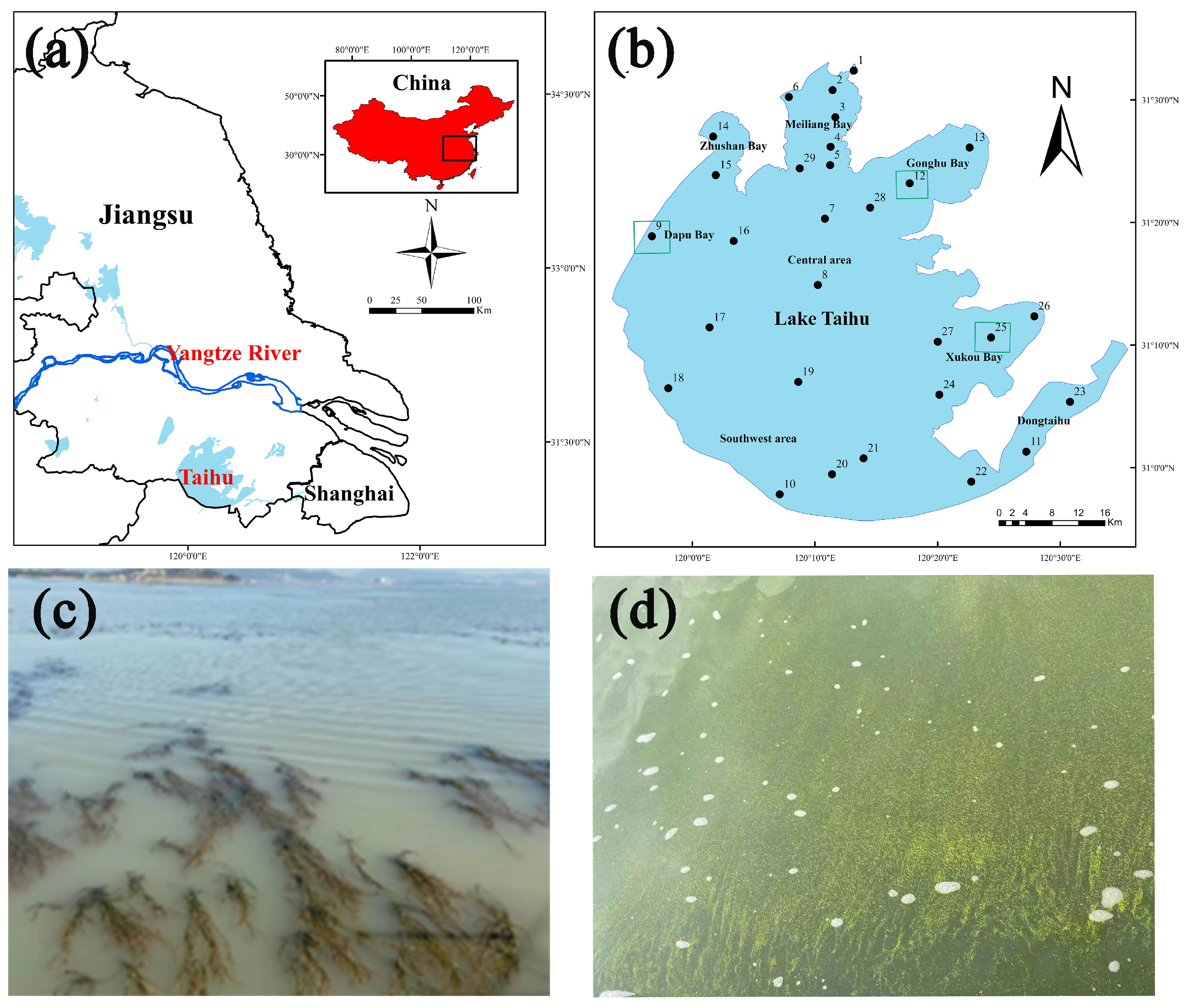
2.2.1. Study Sites

Lake Taihu, which is one of the five largest freshwater lakes in China, is the largest lake in Jiangsu Province (Figure 2a). The southern edge of the lake area is located on the boundary line between Jiangsu and Zhejiang provinces, with a lake area of 2340 km². The annual average water depth is about 2 m, and the lake volume is 4.4 billion cubic meters [28]. Lake Taihu is located in a subtropical zone. The air temperature fluctuates between 3 and 37 °C. The annual average air temperature is 16.0–18.0 °C, and the annual precipitation is 1100–1150 mm. Farmland is the main land-use form surrounding Lake Taihu, accounting for 32.0%, followed by forest land, urban areas, and reservoirs and ponds, accounting for 27.6%, 18.7%, and 14.3%, respectively. The eutrophication of Lake Taihu was aggravated by human-induced nutrient loading. Due to the high degree of eutrophication in Lake Taihu, cyanobacteria have often bloomed during summer in recent years, which seriously affects the water quality [28,29,30,31,32]. Lake Taihu is a sink for nutrients and organic carbon [33] and is a large shallow lake with complex ecological types, including a planktonic algae zone (e.g., Dapu) (Figure 2d), aquatic plant zone (e.g., Xukou) (Figure 2c), and aquatic plant–algae transitional zone (e.g., Gonghu) [28]. These differences lead to the great spatial distribution of water quality and sediment properties. A recent study showed that there were also significant differences in CH₄ emissions from different regions of Lake Taihu. The CH₄ emissions in the algal and aquatic plant areas were significantly higher than that in other lake areas, and the CH₄ emission flux can reach 0.54 ± 0.30 g C m⁻² yr⁻¹, which was seriously underestimated [8]. Thus, we took Lake Taihu as the study site and investigated the CH₄ concentration of surface water at 29 sites in all lake areas (Figure 2b). These 29 sampling sites were distributed evenly across the whole lake based on the lake area. The aim was to observe the differences between these areas and to evaluate the advantages and disadvantages of MIMS and GC in the measurement of dissolved CH₄. In order to evaluate the method of MIMS regarding determining the CH₄ production capacities of sediments, we selected three different types of lake areas, namely, Dapu, Gonghu, and Xukou Bay, and collected undisturbed sediment columns at sites 9, 12, and 25 for laboratory experiments.

2.2.2. Method for Sampling and Data Acquisition

The samples that were used for measuring CH₄ concentrations based on the MIMS method needed to be preserved under non-headspace conditions. Therefore, we collected water samples from a depth about 20 cm below the water surface because directly collecting samples from surface water may sample the ambient air and further affect the subsequent measurement. To compare with the MIMS method, the samples used for determining the CH₄ concentrations based on the HGC method were also collected at the same depth, which was different from the traditional method that directly collected water samples at the water–air interface. The samples that were used for measuring CH₄ concentrations based on the MIMS method were immediately supplemented with 100 μL saturated ZnCl₂ solution to inhibit microbial activity. Samples for the measurement of CH₄ concentration using the HGC method were prepared via equilibration with ambient air. Briefly, 400 mL surface water and 100 mL ambient air were sampled using a 2-way stopcock valve. With the valves closed, the bottle was shaken vigorously for about 5 min to reach equilibrium. The headspace was transferred to a serum bottle that was filled with saturated NaCl solution using two needles [34]. The gas samples were determined using a GC (Model Agilent GC6890N, Agilent Co., CA, USA) that was equipped with a flame ionization detector. It should be noted that the ambient air should be measured to adjust the dissolved gas headspace samples when comparing this method with the MIMS method. However, the ideal dissolved CH₄ concentration after balancing with the air above the surface water is very low (e.g., 3 nmol L⁻¹ under 1.7 ppm in freshwaters in 20 °C). Therefore, for waters with high CH₄ concentrations (e.g., Lake Taihu), the dissolved CH₄ in the water column was primarily from sediments and its self-production in water rather than from the atmosphere, indicating that the CH₄ in the ambient air had little effect on the comparison between the MIMS method and the HGC method if we selected Lake Taihu (a large shallow lake with high CH₄ concentrations) as the sampling area. The water temperature at the sampling sites was measured using a multi-sensor probe (YSI 6600 V2).

2.2.3. Incubation Experiment for Sediment CH₄ Production Rate

CH₄ production rates from sediments were determined via incubation. A large sediment core was used to determine the denitrification and anammox rates based on the continuous flow-through method [35] in our previous studies [32]. Here, we also used a large core to collect sediment with the overlying water from the lake and then separated it into four smaller cores that were placed on the opposite end as the ejector pin (Figure 3). These smaller cores were used to quantify the CH₄ flux at the sediment–water interface. The smaller cores were put into a constant temperature water bath where the temperature was set to the same as the lake water for incubation. Too long of an incubation time may lead to a decrease in the dissolved oxygen (DO) in the water column and may be unable to represent the in situ conditions; therefore, the incubation time was set at 2 days. The concentrations of CH₄ and DO were measured pre-incubation and post-incubation, respectively. Triplicate incubation experiments were conducted at the three sampling sites.

2.2.4. Calculation of CH₄ Production Rates

The CH₄ production rate was calculated using the concentration difference between post-incubation and pre-incubation. The calculation formula was as follows:

$$\mathrm{R}=\left(\mathrm{C}-{\mathrm{C}}_0\right)\times \mathrm{V}/\mathrm{S}/\mathrm{T}$$

(9)

where R is the CH₄ production rate (μmol m⁻² d⁻¹), C₀ is the initial CH₄ concentration (μmol L⁻¹), C is the CH₄ concentration after incubation (μmol L⁻¹), V is the headspace volume (L), S is the basal area of the incubation column (m²), and T is the incubation time (day).

2.3. Comparison with GC Method

We used GC to measure the concentration of CH₄ in the headspace to calculate the concentration of dissolved CH₄ in the samples. The specific calculation formula was as follows:

$${\mathrm{C}}_{\mathrm{water}}^{{\mathrm{CH}}_4}={\mathrm{C}}_{\mathrm{HS}}^{{\mathrm{CH}}_4}\times \left(\mathrm{HRT}+{\mathrm{V}}_{\mathrm{HS}}/{\mathrm{V}}_{\mathrm{water}}\right)$$

(10)

where ${\mathrm{C}}_{\mathrm{water}}^{{\mathrm{CH}}_4}$ represents the methane content in the water before equilibrium (μmol L⁻¹), ${\mathrm{C}}_{\mathrm{HS}}^{{\mathrm{CH}}_4}$ is the CH₄ content in the headspace after equilibrium (μmol L⁻¹), H is Henry’s law constant (mol (L atm)⁻¹), R is the ideal gas constant (L atm (mol K)⁻¹), T is the temperature (K), V_HS is the volume of headspace (L), and V_water is the volume of water (L).

2.4. Statistical Analysis

Linear regression was usually used to detect the relationship between two variables. Here, we used linear regression to show the relationship between the dissolved CH₄ concentration and the CH₄ signal value from MIMS to test whether the MIMS method was reliable. Linear regression was also used to investigate the relationship between dissolved CH₄ concentrations derived from the two different methods. Furthermore, we used the t-test to show the differences in the dissolved CH₄ concentrations derived from the two different methods. If the p-value was greater than 0.05, it indicated no significant differences in the dissolved CH₄ concentrations derived from the two different methods. The linear regression was performed using Origin 8.0, while the t-test was conducted using IBM SPSS 19.0. The figures were produced in Origin 8.0 and ArcGis 10.4.1.

3. Results

3.1. Instrument Response to CH₄ Standards

The standard curves across a range of air saturation (1.7 nM) to 800 μM were highly linear (R² > 0.999; Figure 4b). In addition, under three different salinities, the relationship (Figure 4a) between the CH₄ concentration and signal value were very significant (R² = 0.99813, p < 0.0001 for S = 0; R² = 0.99733, p < 0.0001 for S = 15; R² = 0.99882, p < 0.0001 for S = 30), indicating that salinity had little effect on the accuracy of standard curves.

3.2. Comparison of the MIMS and HGC Methods

In order to determine whether MIMS was reliable, we compared the results with HGC measurements. We selected 29 sites in Lake Taihu and determined the concentration of CH₄ in the surface water using HGC and MIMS. As shown in Figure 5a, the spatial distribution of CH₄ concentrations in the surface water of Lake Taihu was greatly significant, ranging from 0.02 to 0.70 μmol L⁻¹ based on the MIMS method. As a whole, the values obtained from MIMS were consistent with those from HGC, and the linear relationship was also very significant (Figure 5b). Interestingly, we observed that the slope of the fitting curve was greater than 1 and the CH₄ concentrations derived from the MIMS method in many sampling sites were a bit higher than those derived from the HGC method; however, this difference was not significant according to the t-test (p > 0.05).

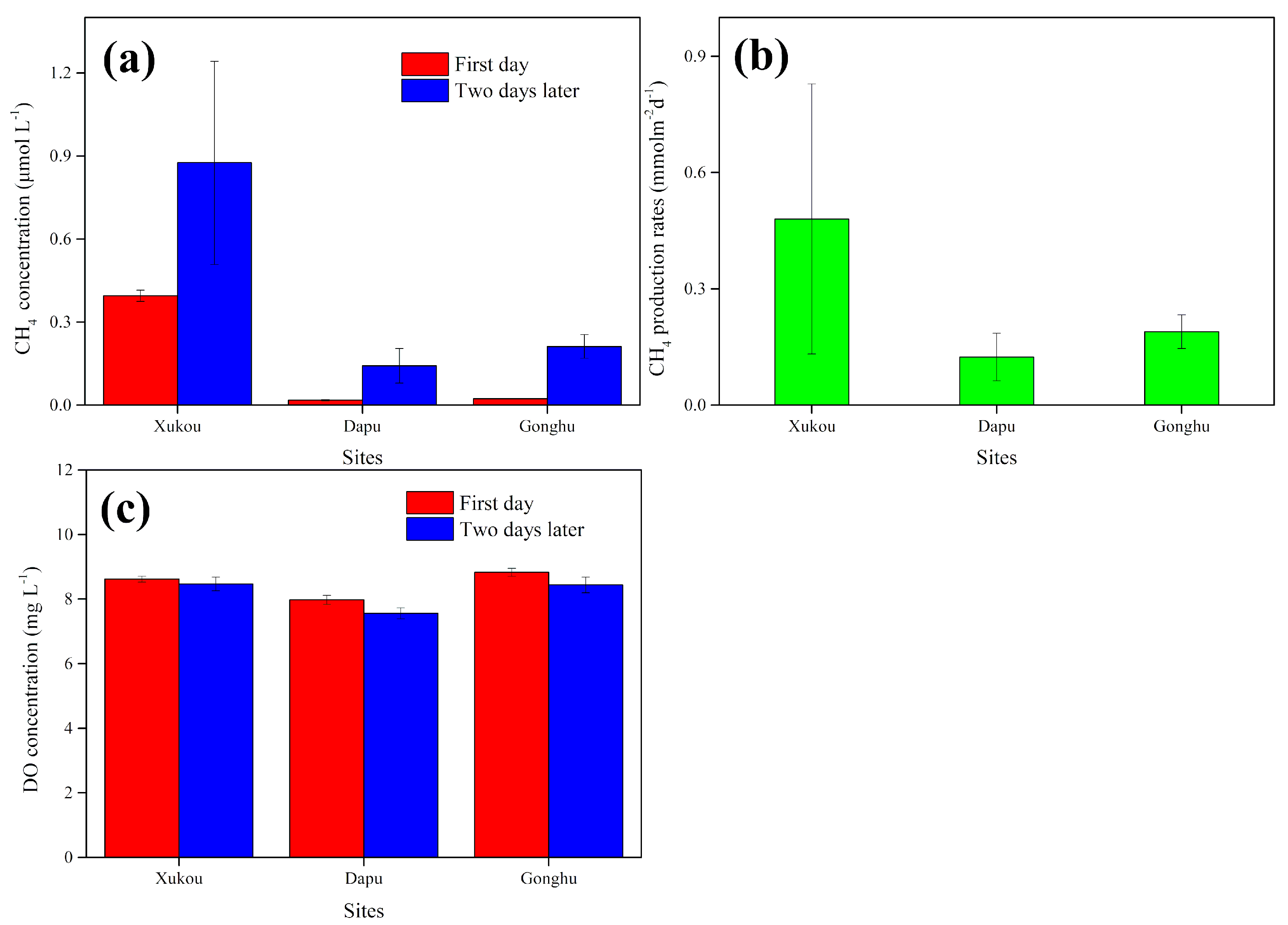
3.3. CH₄ Concentrations and Sediment CH₄ Production Rates in Lake Taihu

In Xukou Bay, the concentrations of CH₄ in surface water were very high, where the highest value was more than 0.63 μmol L⁻¹ (Figure 5a), but it was very low in the center of the lake, which was less than 0.1 μmol L⁻¹ in some sites. We used MIMS to determine the concentration of dissolved CH₄ in a non-headspace incubation experiment, where the results are shown in Figure 6. The dissolved CH₄ accumulations were observed in the cores of Xukou, Dapu, and Gonghu Bays (Figure 6a). The CH₄ production rate in Xukou Bay was the highest, reaching 0.48 ± 0.34 mmol m⁻² d⁻¹, followed by Gonghu and Dapu Bays, with the values of 0.19 ± 0.04 and 0.12 ± 0.06 mmol m⁻² d⁻¹, respectively (Figure 6b). These results indicated that the CH₄ production was obvious in these three sampling sites. Generally, no significant decrease in DO concentrations was observed during the incubation experiment.

4. Discussion

4.1. Assessment of the Analytical Technique

CH₄ detection using MIMS has a 40-year history, where it has been primarily used for microbiological rate measurements under experimental conditions [12]. MIMS has not been the preferred method for environmental water samples; instead, the HGC method is commonplace. Notably, submersible MIMS is incorporated in ROVs for sniffing hydrocarbons in marine systems [36]. Here, we describe a MIMS method that is rapid, precise, sensitive, suited to both trace and highly concentrated samples, and suited to the environmental sampling of water bodies. Contributing to these characteristics is the configuration of the membrane interface. The MIMS used in this study constrains diffusion by imposing a laminar flow across the membrane and having good temperature control of the water flowing across the membrane. This results in sample replicate C.V.s of 0.2% for ion currents (proportional to concentration data) and 0.03% for gas ratios for air gases [14]. CH₄ detection at mass 15 avoids interference from variable O₂ in environmental water samples. However, depending on the mass spectrometer and its settings, there can be mass overlap across adjacent unit masses [37,38]. In the case of CH₄, the mass spectrometer mass resolution may allow O⁺ ions to be detected at mass 15. This can have a significant effect that is observed as a correlation between mass 15 ion currents and oxygen concentration when measuring trace levels of CH₄. The effect can be minimized or eliminated by reducing the resolution parameter of the quadrupole mass spectrometer. Mass 15 is the methyl ion that is also produced by the fragmentation of organic molecules that may pass through the membrane. The use of a liquid nitrogen cryotrap in this study effectively traps all organics that may otherwise interfere at mass 15. Therefore, the mass 15 signal represents an unambiguous measure of CH₄ using the MIMS configuration described here. We demonstrated linearity across low nanomolar to high micromolar concentrations spanning the range expected in nature, including systems experiencing CH₄ ebullition.

4.2. Comparison with HGC

As shown in Figure 5b, the linear relationship between the dissolved CH₄ concentrations derived from the two different methods was significant. However, there were still some small differences. We are confident in the MIMS method because of the satisfactory standard curves (Figure 4). Hence, we speculated that these small differences may have been caused by the potential errors in the HGC method. Headspace equilibration was used to prepare the standard samples for determining CH₄ concentrations using the MIMS method. During the standard sample preparation, the vials were shaken for more than 5 min, which was the same as collecting water samples using the HGC method during the field sampling. The standard curves show that the CH₄ signal values displayed very close relationships for various CH₄ concentrations. Hence, we concluded that the small differences in CH₄ concentrations may not have been caused by incomplete equilibration. Here, we speculated that this small difference may have been due to the following reasons: (1) In the traditional HGC method, the saturated NaCl solution was replaced by the headspace that was from the syringe after the equilibration with lake water. This process was conducted using two gas-tight syringes. However, the injection of the headspace into the serum bottle that was filled with saturated NaCl solution may have easily cause micro-bubbles. Such micro-bubbles may escape with the NaCl solution through another syringe, leading to an underestimate of the dissolved CH₄ concentrations. Furthermore, the higher the CH₄ in the headspace, the higher the underestimate of the dissolved CH₄ concentration will be. (2) Some CH₄ in the headspace may redissolve in the NaCl solution. For a high CH₄ concentration in the headspace, the loss of CH₄ in the headspace caused by redissolution is also high, which may be one of the important reasons for the higher dissolved CH₄ obtained from the MIMS method under high CH₄ concentrations. (3) The transfer of headspace from the syringe to the serum bottle should be conducted carefully. However, during the field samplings, there are too many factors that may affect the transfer, such as the shaking of the boat induced by lake waves due to a high wind speed. Such shaking often appears in large, shallow, and open waters (e.g., Lake Taihu).

In the MIMS method, in addition to the standard samples, the collected field samples do not need headspace processing, and the sampling device is very simple. Only a 12 mL water sample is needed at each site for determination, which means that we can take multiple samples for analysis to reduce the systematic error. It takes about 5 min to determine a sample using the HGC method, but less than 2 min for the MIMS method, which greatly improves the efficiency of sample determination. In addition, the MIMS method can simultaneously measure oxygen, nitrogen, and argon from the same sample vial, which saves a lot of time and labor costs. Furthermore, during the field sampling, the HGC method requires shaking the lake water with air for at least 5 min, while using the MIMS method does not need to make a headspace during sampling and the sampling can be finished within 30 s. For large waters, such as Lake Taihu, sampling from 29 sites across the whole lake using the MIMS method can be finished within half a day. However, it would take at least 2 days if we used the HGC methods. As is well known, the temporal change may lead to the variation in CH₄ concentrations. Therefore, for those who want to collect numerous samples on a short-time scale or want to investigate the spatial distribution of CH₄ concentrations in waters, the MIMS method is more preferred. Additionally, due to the rapid response of the MIMS signal to the variation in CH₄ concentration, MIMS can be used for real-time monitoring of the concentration of CH₄ if desired, which cannot be achieved using the HGC method. It should be noted that the MIMS method also has limitations. Compared with the HGC method, the MIMS method cannot be used to simultaneously determine the concentrations of dissolved carbon dioxide and nitrous oxide since these two gases have almost the same relative atomic mass (~44), which can not be distinguished using MIMS.

4.3. Assessment of the MIMS Method in Lake Taihu

The peak value of the CH₄ concentration measured using the MIMS method appeared in Xukou Bay (Figure 5a), which may have been related to the large number of floating plants and submerged plants there. The degradation of aquatic plants will add a lot of organic carbon to the water and sediments, which is the substrate of CH₄ production [39]. The incubation experiment indicated that Lake Taihu was an important source of CH₄ in summer. A study has shown that submerged macrophytes can significantly promote CH₄ emission from lakes. In our experiment, the CH₄ production rate of sediments in Xukou Bay was the highest, which may be related to the large number of aquatic plants and submerged plants there. Evident CH₄ accumulations also appeared in Dapu and Gonghu Bays. These two lake areas were covered with algae, and the presence of cyanobacteria could significantly promote CH₄ production [40]. Here, we compared our results with those in previous studies, where the results are shown in

Table 3. CH₄ productions from sediments in previous studies.

Location	Type	Method	CH4 Production Rates	Reference
Lake Izunuma	In sediment	Incubation, GC	29.85 mmol m−2 d−1	[41]
Lake Wintergreen	Water–sediment	In situ determination, GC	10–46 mmol m−2 d−1	[42]
Lake Constance	In sediment	Incubation, GC	5–95 mmol m−2 d−1	[43]
Lake Toolik	Water–sediment	Incubation, GC	0.393 mmol m−2 d−1	[44]
Marine basin	Water–sediment	Chamber, GC	2.328 mmol m−2 d−1	[45]
Our study: Lake Taihu	Water–sediment	Incubation, MIMS	0.12–0.48 mmol m−2 d−1

Note: We converted the units of the rate to millimoles per square meter per day.

. Our results were generally lower than those in previous studies, which may have been related to the different properties of sediments; however, the rate of CH₄ release from sediments into the water column was still very high, suggesting that shallow waters (e.g., Lake Taihu) were hotspots for CH₄ production and emission.

5. Conclusions

In this study, we introduced a novel method based upon the MIMS method to determine the dissolved CH₄ concentrations in natural waters. This method was tested in the laboratory and further applied to a large shallow lake, namely, Lake Taihu. Water samples, as well as sediment cores, were collected from Lake Taihu in the summer of 2020 to quantify the CH₄ concentration and CH₄ production rates based on the MIMS method. The results showed that Lake Taihu was an important source of CH₄ in summer. Furthermore, a comparison between the MIMS method with the traditional method (HGC method) was also conducted. Laboratory tests and field sampling showed that our method had significant advantages when measuring dissolved CH₄, including high precision, simple pretreatment, and a fast response. In addition, our method is not only suitable for freshwater lakes, but also other high salinity aquatic ecosystems, such as oceans and saline lakes. We are confident that our MIMS method can replace the traditional HGC method for the determination of dissolved CH₄. Through our method, we could accurately quantify the water–air diffusive flux of CH₄ and determine the CH₄ release rate from sediments to the water column, which provides great convenience regarding studying the fate of CH₄.

References

1. Meinshausen, M.; Meinshausen, N.; Hare, W.; Raper, S.C.B.; Frieler, K.; Knutti, R.; Frame, D.J.; Allen, M.R. Greenhouse-gas emission targets for limiting global warming to 2 °C. Nature 2009, 458, 1158–1162. [Google Scholar] [CrossRef] [PubMed]
2. Ramanathan, V.; Feng, Y. Air pollution, greenhouse gases and climate change: Global and regional perspectives. Atmos. Environ. 2009, 43, 37–50. [Google Scholar] [CrossRef]
3. Montzka, S.A.; Dlugokencky, E.J.; Butler, J.H. Non-CO2 greenhouse gases and climate change. Nature 2011, 476, 43–50. [Google Scholar] [CrossRef] [PubMed]
4. Pall, P.; Aina, T.; Stone, D.A.; Stott, P.A.; Nozawa, T.; Hilberts, A.G.J.; Lohmann, D.; Allen, M.R. Anthropogenic greenhouse gas contribution to flood risk in England and Wales in autumn 2000. Nature 2011, 470, 382–385. [Google Scholar] [CrossRef] [PubMed]
5. Yang, Z.; Grace, J.R.; Lim, C.J.; Zhang, L. Combustion of low-concentration coal bed methane in a fluidized bed. Energy Fuel 2011, 25, 975–980. [Google Scholar] [CrossRef]
6. Deborde, D.; Anschutz, P.; Guérin, F.; Poirier, D.; Marty, D.; Boucher, G.; Thouzeau, G.; Canton, M.; Abril, G.; Jonathan, D.; et al. Methane sources, sinks and fluxes in a temperate tidal Lagoon: The Arcachon lagoon (SW France). Estuar. Coast. Shelf Sci. 2010, 89, 256–266. [Google Scholar] [CrossRef]
7. Qin, X.; Li, Y.; Wan, Y.; Fan, M.; Liao, Y.; Li, Y.; Wang, B.; Gao, Q. Diffusive flux of CH4 and N2O from agricultural river networks: Regression tree and importance analysis. Sci. Total Environ. 2020, 717, 137244. [Google Scholar] [CrossRef]
8. Xiao, Q.; Zhang, M.; Hu, Z.; Gao, Y.; Hu, C.; Liu, C.; Liu, S.; Zhang, Z.; Zhao, J.; Xiao, W.; et al. Spatial variations of methane emission in a large shallow eutrophic lake in subtropical climate. J. Geophys. Res.-Biogeosci. 2017, 122, 1597–1614. [Google Scholar] [CrossRef]
9. Lomond, J.S.; Tong, A.Z. Rapid analysis of dissolved methane, ethylene, acetylene and ethane s.ing partition coefficients and headspace-gas chromatography. J. Chromatogr. Sci. 2011, 49, 469–475. [Google Scholar] [CrossRef] [Green Version]
10. Villa, J.A.; Smith, G.J.; Ju, Y.; Renteria, L.; Angle, J.C.; Arntzen, E.; Harding, S.F.; Ren, H.; Chen, X.; Sawyer, A.H.; et al. Methane 445 and nitrous oxide porewater concentrations and surface fluxes of a regulated river. Sci. Total Environ. 2020, 715, 136920. [Google Scholar] [CrossRef]
11. Smith, R.L.; Böhlke, J.K. Methane and nitrous oxide temporal and spatial variability in two U.S. Midwestern streams containing high nitrate concentrations. Sci. Total Environ. 2019, 685, 574–588. [Google Scholar] [CrossRef]
12. Carlsen, H.N.; Joergensen, L.; Degn, H. Inhibition by ammonia of methane utilization in Methylococcus capsulatus (Bath). Appl. Microbiol. Biotechnol. 1991, 35, 124–127. [Google Scholar] [CrossRef]
13. Lauritsen, F.R.; Kotiaho, T. Advances in membrane inlet mass spectrometry (MIMS). Rev. Anal. Chem. 1996, 15, 237–264. [Google Scholar] [CrossRef]
14. Kana, T.M.; Darkangelo, C.; Hunt, M.D.; Oldham, J.B.; Bennett, G.E.; Cornwell, J.C. Membrane inlet mass spectrometer for rapid high-precision determination of N2, O2, and Ar in environmental water samples. Anal. Chem. 1994, 66, 4166–4170. [Google Scholar] [CrossRef]
15. Hou, L.; Yin, G.; Liu, M.; Zhou, J.; Zheng, Y.; Gao, J.; Zong, H.; Yang, Y.; Gao, L.; Tong, C. Effects of sulfamethazine on denitrification and the associated N2O release in estuarine and coastal sediments. Environ. Sci. Technol. 2014, 49, 326–333. [Google Scholar] [CrossRef] [PubMed]
16. Zhao, Y.; Xia, Y.; Ti, C.; Shan, J.; Li, B.; Xia, L.; Yan, X. Nitrogen removal capacity of the river network in a high nitrogen loading region. Environ. Sci. Technol. 2015, 49, 1427–1435. [Google Scholar] [CrossRef] [PubMed]
17. Bižić, M.; Klintzsch, T.; Ionescu, D.; Hindiyeh, M.Y.; Günthel, M.; Muro-Pastor, A.M.; Eckert, W.; Eckert, T.; Keppler, F.; Keppler, H.P. Aquatic and terrestrial cyanobacteria produce methane. Sci. Adv. 2020, 6, 5343. [Google Scholar] [CrossRef] [Green Version]
18. Kana, T.M.; Weiss, D.L. Comment on “Comparison of Isotope Pairing and N2:Ar Methods for Measuring Sediment Denitrification” By B. D. Eyre, S. Rysgaard, T. Dalsgaard, and P. Bondo Christensen. 2002. Estuaries 25:1077–1087. Estuaries 2004, 25, 173–176. [Google Scholar] [CrossRef]
19. Wanninkhof, R. Relationship between wind speed and gas exchange over the ocean revisited. J. Geophys. Res. Ocean. 1992, 97, 7373–7382. [Google Scholar] [CrossRef]
20. Zhou, Y.; Xiao, Q.; Yao, X.; Zhang, Y.; Zhang, M.; Shi, K.; Lee, X.; David, C.P.; Qin, B.; Robert, G.M.S.; et al. Accumulation of terrestrial dissolved organic matter potentially enhances dissolved methane levels in eutrophic Lake Taihu, China. Environ. Sci. Technol. 2018, 52, 10297–10306. [Google Scholar] [CrossRef]
21. Liu, R.M.; Annette, H.; Fazil, O.G.; Pierre, Y.F.; Janusz, D. Methane concentration profiles in a lake with a permanently anoxic hypolimnion (Lake Lugano, Switzerland-Italy). Chem. Geol. 1996, 133, 201–209. [Google Scholar] [CrossRef]
22. Gar’kusha, D.N.; Fedorov, Y.A. Distribution of methane concentration in coastal areas of the Gulf of Petrozavodsk, Lake Onega. Water Resour. 2015, 42, 331–339. [Google Scholar] [CrossRef]
23. Juutinen, S.; Rantakari, M.; Kortelainen, P.; Huttunen, J.T.; Larmola, T.; Alm, J.; Martikainen, P.J. Methane dynamics in different boreal lake types. Biogeosciences 2009, 6, 209–223. [Google Scholar] [CrossRef] [Green Version]
24. Castro-Morales, K.; Macías-Zamora, J.V.; Canino-Herrera, S.R.; Burke, R.A. Dissolved methane concentration and flux in the coastal zone of the Southern California Bight-Mexican sector: Possible influence of wastewater. Estuar. Coast. Shelf Sci. 2014, 144, 65–74. [Google Scholar] [CrossRef]
25. Gilbert, B.; Frenzel, P. Methanotrophic bacteria in the rhizosphere of rice microcosms and their effect on porewater methane concentration and methane emission. Biol. Fertil. Soils 1995, 20, 93–100. [Google Scholar] [CrossRef]
26. Tan, Y.; Wang, D.; Deng, H.; Li, Y.; Yu, Z.; Chen, Z. Methane and nitrous oxide dissolved concentration and emission flux of plain river network in winter. Sci. Sin. Chim. 2013, 43, 919–929. [Google Scholar]
27. Yin, G.; Hou, L.; Liu, M.; Liu, Z.; Gardner, W.S. A novel membrane inlet mass spectrometer method to measure 15NH4+ for isotope-enrichment experiments in aquatic ecosystems. Environ. Sci. Technol. 2014, 48, 9555–9562. [Google Scholar] [CrossRef]
28. Qin, B.; Xu, P.; Wu, Q.; Luo, L.; Zhang, Y. Environmental issues of Lake Taihu, China. Hydrobiologia 2007, 581, 3–14. [Google Scholar] [CrossRef]
29. Qin, B.; Zhu, G.; Gao, G.; Zhang, Y.; Li, W.; Paerl, H.W.; Carmichael, W.W. A drinking water crisis in Lake Taihu, China: Linkage to climatic variability and lake management. Environ. Manag. 2011, 45, 105–112. [Google Scholar] [CrossRef] [PubMed]
30. Hu, C.; Lee, Z.; Ma, R.; Yu, K.; Li, D.; Shang, S. Moderate resolution imaging spectroradiometer (MODIS) observations of cyanobacteria blooms in Taihu Lake, China. J. Geophys. Res.-Ocean. 2010, 115, C04002. [Google Scholar] [CrossRef] [Green Version]
31. Zhao, F.; Zhan, X.; Xu, H.; Zhu, G.; Zou, W.; Zhu, M.; Kang, L.; Guo, Y.; Zhao, X.; Wang, Z.; et al. New insights into eutrophication management: Importance of temperature and water residence time. J. Environ. Sci. 2022, 111, 229–239. [Google Scholar] [CrossRef]
32. Zhao, F.; Xu, H.; Zhan, X.; Zhu, G.; Guo, Y.; Kang, L.; Zhu, M. Spatial differences and influencing factors of denitrification and ANAMMOX rates in spring and summer in Lake Taihu. Environ. Sci. 2021. [Google Scholar] [CrossRef]
33. Zhou, Y.; Yao, X.; Zhang, Y.; Zhang, Y.; Shi, K.; Tang, X.; Qin, B.; Podgorski, D.C.; Brookes, J.D.; Jeppesen, E. Response of dissolved organic matter optical properties to net inflow runoff in a large fluvial plain lake and the connecting channels. Sci. Total Environ. 2018, 639, 876–887. [Google Scholar] [CrossRef] [PubMed]
34. Donis, D.; Flury, S.; Stöckli, A.; Spangenberg, J.E.; Vachon, D.; McGinnis, D.F. Full-scale evaluation of methane production under oxic conditions in a mesotrophic lake. Nat. Commun. 2017, 8, 1–12. [Google Scholar] [CrossRef] [PubMed] [Green Version]
35. Risgaard-Petersen, N.; Nielsen, L.P.; Blackburn, T.H. Simultaneous measurement of benthic denitrification, with the isotope pairing technology and the N2 flux method in a continuous flow-through system. Water Res. 1998, 32, 3371–3377. [Google Scholar] [CrossRef]
36. Mcmutrtry, G.M.; Wiltshire, J.C.; Bossuyt, A. Hydrocarbon seep monitoring using in situ deep sea mass spectrometry. In Europe Oceans; IEEE: Piscataway, NJ, USA, 2005. [Google Scholar]
37. Eyre, B.D.; Rysgaard, S.; Dalsgaard, T.; Christensen, P.B. Comparison of isotope pairing and N2: Ar methods for measuring sediment denitrification-Assumptions, modifications, and implications. Estuaries 2020, 25, 1077–1087. [Google Scholar] [CrossRef]
38. Lunstrum, A.; Aoki, L.R. Oxygen interference with membrane inlet mass spectrometry may overestimate denitrification rates calculated with the isotope pairing technique. Limnol. Oceangr. Methods 2016, 14, 425–431. [Google Scholar] [CrossRef] [Green Version]
39. Horruitiner, C.D.; Varner, R.K.; Palace, M.W.; Johnson, J.E.; Wik, M.; Lungren, D.J. Examining the Role of Aquatic Vegetation in Methane Production: Examples from a Shallow High Latitude Lake in Abisko, Sweden. Available online: https://agu.confex.com/agu/fm15/webprogram/Paper83308.html (accessed on 26 September 2021).
40. William, E.W.; James, J.C.; Stuart, E.J. Effects of algal and terrestrial carbon on methane production rates and methanogen community structure in a temperate lake sediment. Freshw. Biol. 2012, 57, 949–955. [Google Scholar]
41. Lay, J.; Miyahara, T.; Noike, T. Methane release rate and methanogenic bacterial populations in lake sediments. Water Res. 1996, 30, 901–908. [Google Scholar] [CrossRef]
42. Strayer, R.F.; Tiedje, J.M. In situ methane production in a small, hypereutrophic, hard-water lakes: Loss of methane from sediments by vertical diffusion and ebullition. Limnol. Oceanogr. 1978, 23, 1201–1206. [Google Scholar] [CrossRef]
43. Thebrath, B.; Rothfuss, F.; Whiticar, M.J.; Conrad, R. Methane production in littoral sediment of Lake Constance. FEMS Microbiol. Ecol. 1993, 102, 279–289. [Google Scholar] [CrossRef]
44. Gentzel, T.; Hershey, A.E.; Rublee, P.A.; Whalen, S.C. Net sediment production of methane, distribution of methanogens and methane-oxidizing bacteria, and utilization of methane-derived carbon in an arctic lake. Inland Waters 2012, 2, 77–88. [Google Scholar] [CrossRef]
45. Martens, C.S.; Klump, J.V. Biogeochemical cycling in an organic-rich coastal marine basin—I. Methane sediment-water exchange processes. Geochim. Cosmochim. Acta 1980, 44, 471–536. [Google Scholar] [CrossRef]
Figure 1. The diagram of the MIMS system.
Water 13 02699 g001
Figure 2. (a) The location of Lake Taihu in Jiangsu Province; (b) the specific distribution of sampling sites in Lake Taihu, where the black spots are 29 sites for surface gas collection and the green square frames are 3 points for collecting sediments; (c,d) images of an aquatic-plant-covered area and an algal-covered area, respectively.
Water 13 02699 g002
Figure 3. Schematic diagram of the sampling device.
Water 13 02699 g003
Figure 4. (a) Fitting curves using the CH4 concentration as the abscissa and signal values as the ordinate under different salinities (0, 15, and 30) at 20 °C. The black, red, and blue curves represent the fitting curves at salinities of 0, 15, and 30, respectively. (b) Fitting curve for high CH4 concentrations of standard samples at 20 °C.
Water 13 02699 g004
Figure 5. Relationship between the CH4 concentrations derived from MIMS and CH4 concentrations based on GC. (a) represents the differences between GC and MIMS, (b) is the fitting curve between GC and MIMS.
Water 13 02699 g005
Figure 6. (a) The concentration of dissolved CH4 in the incubation experiment, where red means before incubation and blue means after incubation; (b) CH4 production rates of sediments; (c) the DO concentrations in the incubation experiment.
Water 13 02699 g006