A Modified Bare Soil Index to Identify Bare Land Features during Agricultural Fallow-Period in Southeast Asia Using Landsat 8

Abstract

Bare soil is a critical element in the urban landscape and plays an essential role in urban environments. Yet, the separation of bare soil and other land cover types using remote sensing techniques remains a significant challenge. There are several remote sensing-based spectral indices for barren detection, but their effectiveness varies depending on land cover patterns and climate conditions. Within this research, we introduced a modified bare soil index (MBI) using shortwave infrared (SWIR) and near-infrared (NIR) wavelengths derived from Landsat 8 (OLI—Operational Land Imager). The proposed bare soil index was tested in two different bare soil patterns in Thailand and Vietnam, where there are large areas of bare soil during the agricultural fallow period, obstructing the separation between bare soil and urban areas. Bare soil extracted from the MBI achieved higher overall accuracy of about 98% and a kappa coefficient over 0.96, compared to bare soil index (BSI), normalized different bare soil index (NDBaI), and dry bare soil index (DBSI). The results also revealed that MBI considerably contributes to the accuracy of land cover classification. We suggest using the MBI for bare soil detection in tropical climatic regions.

1. Introduction

Remote sensing and satellite imagery have been widely utilized for monitoring land and environmental changes, including urban expansion [1,2,3], deforestation [4,5,6], climate change impacts [7,8], wildfire damage [9,10], and other natural and anthropogenic dynamics. Presently, there are diverse high-resolution satellites which positively support urban studies, such as HyMap [11], Worldview [12], SPOT [13,14], and Sentinel-2 [15,16]. An integration of Sentinel-2 and Sentinel-1, a free-of-charge Synthetic Aperture Radar (SAR) sensor, has potential for urban mapping [17,18]. Yet, the major limitations of these observation data are data-acquired costs and time of coverage, especially for urban expansion studies, which are often considered over a long-term period. The cost per scene for commercial satellites is costly relative to the income of developing countries. The freely accessible data with fine resolution such as the Sentinel mission has only been available since 2015. Therefore, Landsat data (i.e., 4, 5, 7-ETM, and 8-OLI) are commonly used in numerous studies worldwide since its data cover nearly 50 years consecutively [19]. With medium multispectral resolution and powerful thermal infrared (TIR) sensors, Landsat data are applied for monitoring urban expansion and surface temperature, an essential parameter in the urban environment [20,21,22,23,24].

The presence of bare soil in peri-urban and countryside regions has posed difficulties for accurate classification of urban land covers. This is partly because bare soil and urban features have relatively similar spectral characteristics [25]. This confusion could be limited by using settlement products (e.g., World Settlement Footprint-WSF [26], Global Human Settlement Layer-GHSL [27,28]) to mask out urban areas. Data continuity is a disadvantage since these data are solely aggregated for a few certain time hooks. Multitemporal data are a potential approach to detect bare soil since agricultural bare soil is seasonal, whereas urban features are permanent. Yet, applying multitemporal data in the tropical region is relatively difficult due to data loss during the rainy season when the cloud cover rate is up to 85–95% [29,30]. Bare soil detection, therefore, is still a challenging task.

The bare soil includes fallow agricultural land during the fallow period of cultivation-land preparation time of transition between two crops—and available land after the land clearance process or pre-urbanized parcels [31]. In some urban areas, the presence and extension of bare soil are closely related to dust storm frequency, especially in desert and arid climate regions [32,33,34]. Besides, barren land without vegetation is vulnerable to sediment transport, soil erosion, and landslides [35,36,37]. Such fallow land is essential because of its relatively lower heat capacity relative to other land cover types, inducing high temperatures over its land surface. It is, therefore, vital to classify bare soil in urban studies, mainly when the urban heat island (UHI) is assessed in various temporal and spatial scales [38]. The dynamics of land cover changes and inaccuracy in classifying bare soil leads to inadequate assessment of the heat harshness in inner city areas.

Barren land is often misclassified as built-up areas and vice versa. We may face an “unrealistic urbanization” because the classified urban areas are actually bare soil areas. Consequently, urban development rates and developing tendencies might be erroneously assessed in the very first step of urban planning. Once barren land is efficiently differentiated from built-up land, it improves urban expansion assessment and helps contribute to other developments such as agricultural management. For instance, there were 238,276 hectares of rice cultivation in the Vietnamese Mekong Delta damaged during the severe drought and salinity intrusion in the dry season of 2015–2016 [39]. Such damage could be assessed by monitoring the fallow land areas. An identical evaluation is applicable for aquaculture, such as allocating fallow shrimp ponds [40,41]. Therefore, bare soil monitoring is crucial for land use planning and agricultural practices, and policymaking.

Scholars worldwide have proposed many spectral indices derived from Landsat to discriminate bare soil from other lands (

Table 1. Bare soil indices derived from Landsat imagery.

Index	Data	Formula	Case Study	References
Bare soil index	Landsat TM, ETM, 8 (OLI)	$\mathrm{B}\mathrm{S}\mathrm{I}=\frac{\left(\mathrm{S}\mathrm{W}\mathrm{I}\mathrm{R}2+\mathrm{R}\right)-\left(\mathrm{N}\mathrm{I}\mathrm{R}+\mathrm{B}\right)}{\left(\mathrm{S}\mathrm{W}\mathrm{I}\mathrm{R}2+\mathrm{R}\right)+\left(\mathrm{N}\mathrm{I}\mathrm{R}+\mathrm{B}\right)}$	The Swiss Plateau, Switzerland	[48]
Bare soil index 1	Landsat TM	$\mathrm{B}\mathrm{S}\mathrm{I}1=\frac{\left(\mathrm{S}\mathrm{W}\mathrm{I}\mathrm{R}1+\mathrm{R}\right)-\left(\mathrm{N}\mathrm{I}\mathrm{R}+\mathrm{B}\right)}{\left(\mathrm{S}\mathrm{W}\mathrm{I}\mathrm{R}1+\mathrm{R}\right)+\left(\mathrm{N}\mathrm{I}\mathrm{R}+\mathrm{B}\right)}$	Guangdong, China	[34]
Bare soil index 2	Landsat TM	$\mathrm{B}\mathrm{S}\mathrm{I}2=100\times \sqrt{\frac{\mathrm{S}\mathrm{W}\mathrm{I}\mathrm{R}2-\mathrm{G}}{\mathrm{S}\mathrm{W}\mathrm{I}\mathrm{R}2+\mathrm{G}}}$	South Africa	[47]
Bare soil index 3	Landsat TM, ETM	$\mathrm{B}\mathrm{S}\mathrm{I}3=\frac{\left(\mathrm{S}\mathrm{W}\mathrm{I}\mathrm{R}1+\mathrm{R}\right)-\left(\mathrm{N}\mathrm{I}\mathrm{R}+\mathrm{B}\right)}{\left(\mathrm{S}\mathrm{W}\mathrm{I}\mathrm{R}1+\mathrm{R}\right)+\left(\mathrm{N}\mathrm{I}\mathrm{R}+\mathrm{B}\right)}\times 100+100$	Iran	[45]
Normalized difference soil index 1	Landsat TM	$\mathrm{N}\mathrm{D}\mathrm{S}\mathrm{I}1=\frac{\mathrm{S}\mathrm{W}\mathrm{I}\mathrm{R}1-\mathrm{N}\mathrm{I}\mathrm{R}}{\mathrm{S}\mathrm{W}\mathrm{I}\mathrm{R}1+\mathrm{N}\mathrm{I}\mathrm{R}}$	−	[46]
Normalized difference soil index 2	Landsat TM	$\mathrm{N}\mathrm{D}\mathrm{S}\mathrm{I}2=\frac{\mathrm{S}\mathrm{W}\mathrm{I}\mathrm{R}2-\mathrm{G}}{\mathrm{S}\mathrm{W}\mathrm{I}\mathrm{R}2+\mathrm{G}}$	Milwaukee and Waukesha, US	[50]
Normalized difference bareness index	Landsat TM, ETM	$\mathrm{N}\mathrm{D}\mathrm{B}\mathrm{a}\mathrm{I}=\frac{\mathrm{S}\mathrm{W}\mathrm{I}\mathrm{R}1-\mathrm{T}\mathrm{I}\mathrm{R}}{\mathrm{S}\mathrm{W}\mathrm{I}\mathrm{R}1+\mathrm{T}\mathrm{I}\mathrm{R}}$	Northern coastal China	[52]
Bareness Index	Landsat TM	$\mathrm{B}\mathrm{I}=\left(\mathrm{R}+\mathrm{S}\mathrm{W}\mathrm{I}\mathrm{R}1-\mathrm{N}\mathrm{I}\mathrm{R}\right)$	Beijing, China	[44]
Enhanced built-Up and bareness index	Landsat ETM	$\mathrm{E}\mathrm{B}\mathrm{B}\mathrm{I}=\frac{\mathrm{S}\mathrm{W}\mathrm{I}\mathrm{R}1-\mathrm{N}\mathrm{I}\mathrm{R}}{10\sqrt{\mathrm{S}\mathrm{W}\mathrm{I}\mathrm{R}1+\mathrm{T}\mathrm{I}\mathrm{R}}}$	Bali, Indonesia	[31]
Modified normalized difference soil index	Landsat 8 (OLI)	$\mathrm{M}\mathrm{N}\mathrm{D}\mathrm{S}\mathrm{I}=\frac{\mathrm{S}\mathrm{W}\mathrm{I}\mathrm{R}2-\mathrm{P}\mathrm{A}\mathrm{N}}{\mathrm{S}\mathrm{W}\mathrm{I}\mathrm{R}2+\mathrm{P}\mathrm{A}\mathrm{N}}$	Dehradun, India	[54]
Normalized difference bare land index	Landsat TM, 8 (OLI)	$\mathrm{N}\mathrm{B}\mathrm{L}\mathrm{I}=\frac{\mathrm{R}-\mathrm{T}\mathrm{I}\mathrm{R}}{\mathrm{R}+\mathrm{T}\mathrm{I}\mathrm{R}}$	Wuhan, China	[53]
Dry bare-soil index	Landsat 8 (OLI)	$\mathrm{D}\mathrm{B}\mathrm{S}\mathrm{I}=\frac{\mathrm{S}\mathrm{W}\mathrm{I}\mathrm{R}1-\mathrm{G}}{\mathrm{S}\mathrm{W}\mathrm{I}\mathrm{R}1+\mathrm{G}}-\frac{\mathrm{N}\mathrm{I}\mathrm{R}-\mathrm{R}}{\mathrm{N}\mathrm{I}\mathrm{R}+\mathrm{R}}$	Kurdistan, Iraq	[49]

R: red wavelength, G: green wavelength, B: blue wavelength, NIR: near-infrared, SWIR1: shortwave infrared band 5 (Landsat TM/ETM) and band 6 (Landsat 8), SWIR2: shortwave infrared band 6 (Landsat TM/ETM) and band 7 (Landsat 8), PAN: panchromatic band 8 (Landsat ETM/8), TIR: thermal infrared band 6 (Landsat TM/ETM) and band 10 (Landsat 8).

). Generally, bare soil indices are constructed from various Landsat wavelengths from visible to near-infrared (NIR) and shortwave infrared (SWIR) wavelengths with a two, three, and four band combined index. Koroleva et al. [42] proposed an approach to separate bare soil applying the Red-NIR spectral space, which is a principal basis in determining soil type [43]. Although bare soil occupies an ellipse-shaped area on the Red-NIR plot, it is smaller than the vegetation area [42]. It may lead to difficulty in discrimination between bare soil and other land cover types in general. Lin et al. [44] proposed a non-ratio index, bareness index (BI), for urban feature extraction in general from band Red, NIR, and SWIR1 (1.57–1.65 μm). However, this index has limited ability to separate bare soil from built-up areas [44]. Likewise, enhanced built-up and bareness index (EBBI) was introduced to detect urban features and bare soil, but its differentiation ability is inadequate [31]. Bare soil features are also not distinguished from built-up features in bare soil index 3 (BSI3) [45] and normalized difference soil index 1 (NDSI1) [46]. For the bare soil indices, including BSI2 [47], BSI [48], BSI1 [34], and dry bare soil index (DBSI) [49], barren land and urban area cannot be separated due to their similarities and overlapping thresholding values. Whether it is a two-band or four-band ratio, bare soil parcels were differentiated less clearly by these bare soil indices due to their limited capability. DBSI was initially proposed for arid climatic regions (i.e., Iraq), and applying DBSI in humid regions is therefore inappropriate. Deng et al. [50] introduced a normalized difference soil index (NDSI2) in an attempt to highlight bare soil information by reversing the modified normalized difference water index (MNDWI) [51] based on the high reflectance of bare soil in the shortwave infrared wavelength. Yet, the NDSI2 is able to detect large and dry bare soil parcels while small and sparse parcels are often neglected. Thermal infrared wavelength (TIR) has been utilized to facilitate bare soil detection; for example, normalized difference bareness index (NDBaI) [52] and normalized difference bare land index (NBLI) [53]. The performance of NDBaI and NBLI is relatively high compared to other barren indices. Nevertheless, the disadvantage of using thermal infrared-based is low resolution originating from TIR (i.e., 60 m in Landsat TM/ETM, 100 m in Landsat 8). By using panchromatic (PAN) images with better spatial resolution (i.e., 15 m) and SWIR2 (2.11–2.29 μm), the modified normalized difference soil index (MNDSI) overcomes the limitation of low resolution on NDBaI. Besides, MNDSI shows excellent discrimination between urban areas and bare soil in a comparatively hot area like Dehradun (India) [54]. It is also the case that most of these indices were firstly designed for temperate climate and high latitude regions. It is well known that the barren index’s performance is significantly affected by climate patterns [49]. Hence it is not suitable for the tropical monsoon climate with different bare soil patterns (i.e., homogeneous versus sparse bare soil, see Section 2.1).

This paper aims to introduce a more accurate bare soil index to support long-term studies related to land cover classification using Landsat images in the tropics. Firstly, we introduce a new bare soil index to improve the discrimination between bare soil and other land covers in finer resolution using a spectral index derived from Landsat 8 imagery. Subsequently, we assessed the proposed modified bare soil index’s performance in two test sites and made further comparisons with three other available bare soil indices.

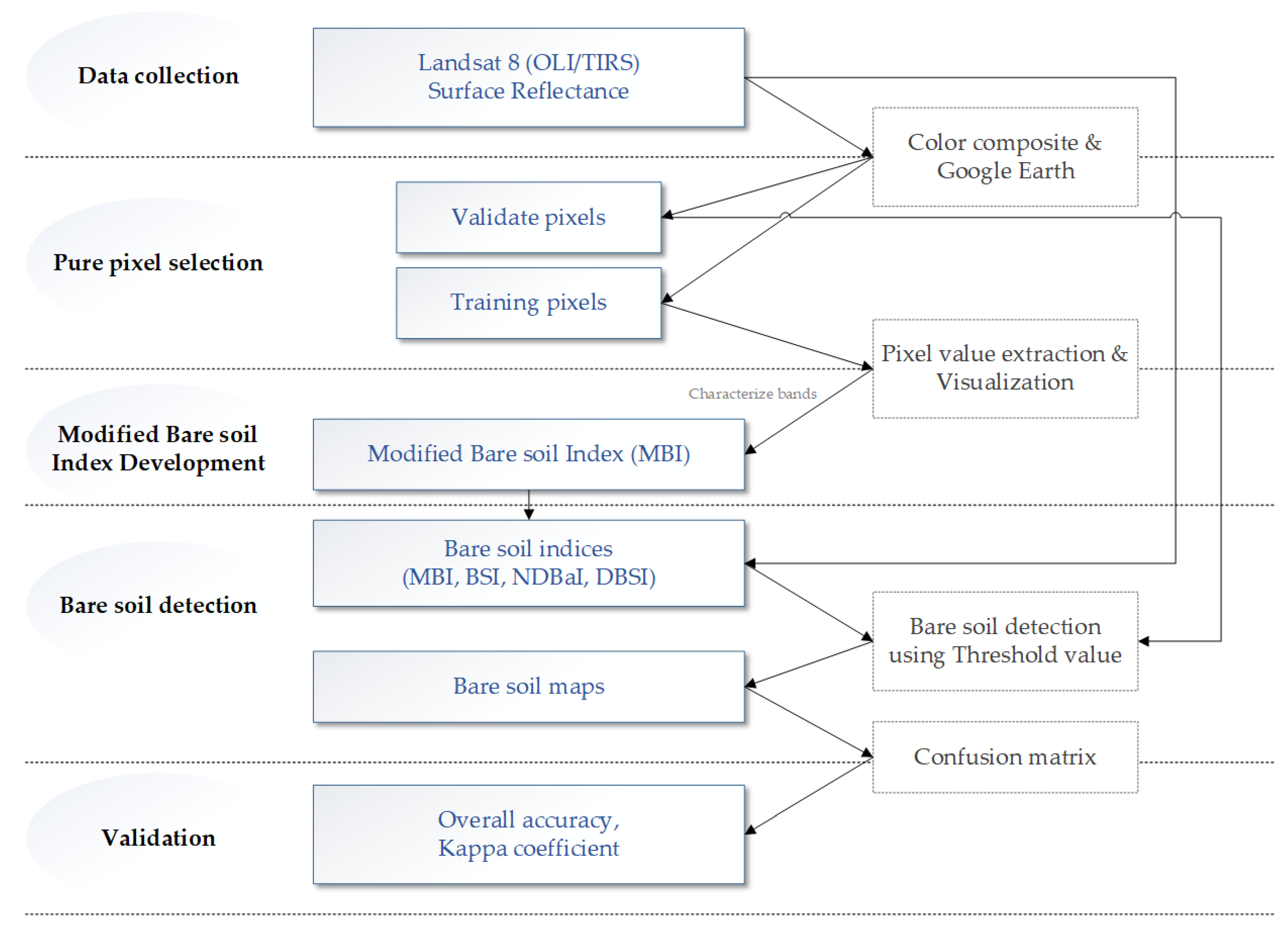
2. Materials and Methods

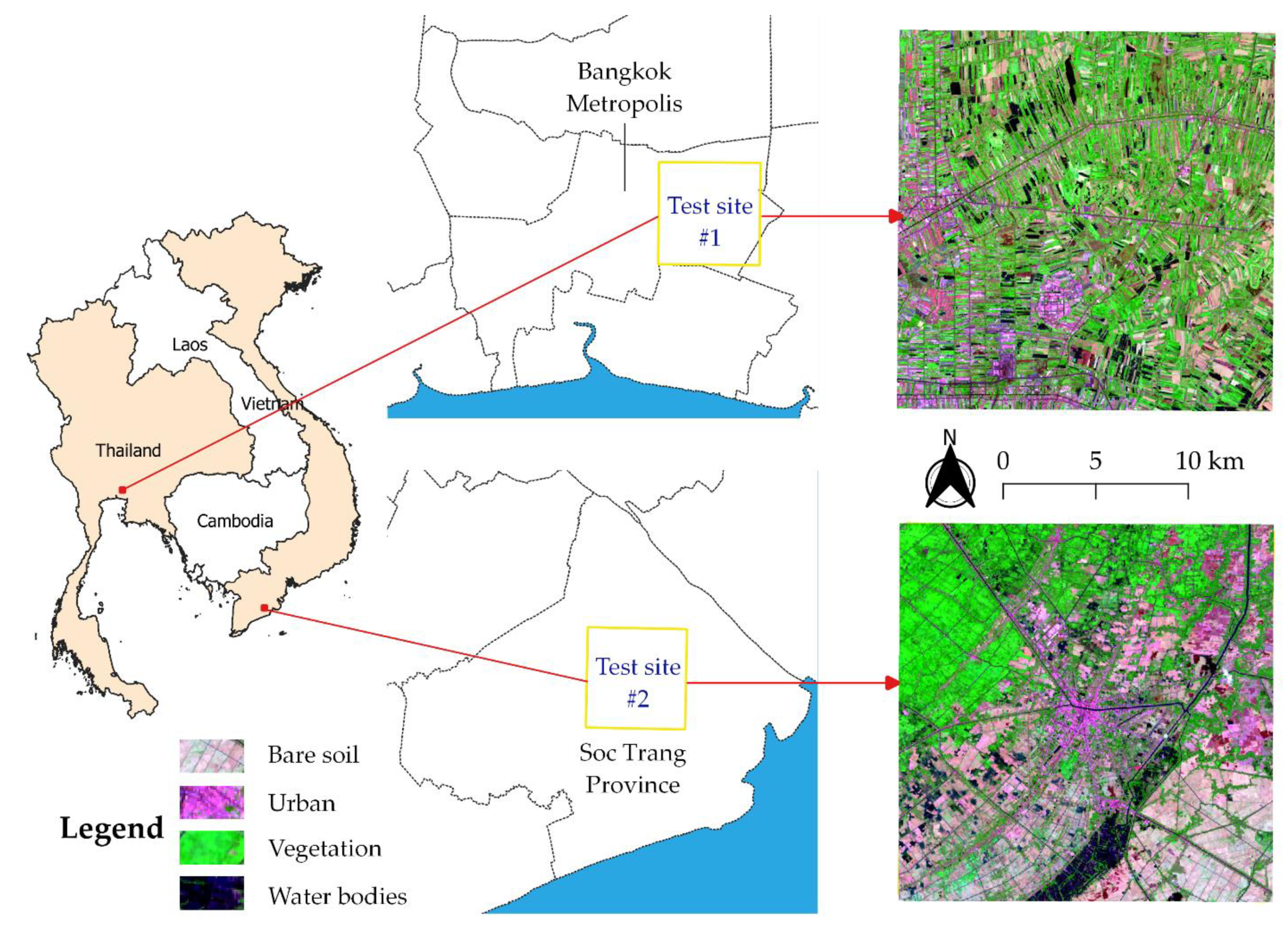
Figure 1 presents a flowchart that describes the procedures of development and validation of the modified bare soil index from data used to output. Each step is discussed in detail below.

2.1. Test Sites

We chose the eastern Bangkok metropolis (Thailand) as the first test site (test site #1) because this is a semi-urban region with heterogeneous urban and annual agricultural landscapes, which become seasonal bare land in the fallow period [55] (Figure 2). The concentrated and smaller-size residential areas are interspersed with the fields due to the suburbanization process [56]. The second site (test site #2) is located in central Soc Trang province, a local city in the Vietnamese Mekong Delta, where most agricultural land is double-cropped rice or a rain-fed rice system [57]. The immense paddy fields become seasonal bare soil during the dry and salinity intrusion periods. Both test sites are located in flat low plains and distributed over the Gley soil (Gleysols-GL) based on the World Reference Base for Soil Resources (WRB) [58,59]. Specifically, the test sites are square with a 20 km edge and dominated by four major land cover types (i.e., bare soil, built-up, vegetation, and water bodies).

2.2. Data

Two Landsat 8 (OLI/TIRS) scenes were collected from the US Geological Survey (USGS) website (https://earthexplorer.usgs.gov (accessed on 26 August 2020)) The image covering Bangkok metropolitan (Thailand) was captured on 19 February 2020 (WRS-2 path/row: 129/50), and the other image was also in the dry season of 2020 in Soc Trang province (Vietnam) on 25 February with path 125 and row 53. All images are Level-2 data (surface reflectance) with a cloud cover rate of less than 0.5%, minimizing atmospheric effects for further analyses.

Compared to other Landsat satellites, Landsat-8 was retrofitted with coastal aerosol and cirrus bands for cloud-related studies. The main drawback of Landsat 8 data is a low resolution of thermal infrared bands, about 100 m compared to 60 m in Landsat 7, affecting the accuracy of urban bare soil detection using the thermal band [60,61]. The thermal infrared band therefore was eliminated from potential indices, whereas the remaining bands were preferred to maintain the index resolution at 30 m. Shortwave infrared (SWIR) bands were especially considered since these bands can penetrate thin clouds and discriminate vegetation and soil [62,63].

2.3. Modified Bare Soil Index

Figure 3a shows the reflectance properties of four land cover types, which are visualized by 4000 training pixels on both sites. This graph also shows profiles of bare soil and built-up cover that are relatively similar and lead to a challenge in urban bare soil separation in urban studies. These two features’ reflectance values vary depending on to visible wavelength, but urban features reflect more energy in this wave range. In contrast, bare soil reflects more near infrared (0.85–0.88 μm) and shortwave infrared 1 (SWIR1: 1.57–1.65 μm), band 5 and band 6 on Landsat 8, respectively. Bare soil tends to absorb energy in shortwave infrared 2 (SWIR2: 2.11–2.29 μm) against urban features.

On the other hand, water attracts most of the energy from the visible to the infrared spectrum, especially for the SWIR1 and SWIR2 channels. Vegetation absorbs these SWIR wavelengths, whereas NIR energy is mostly returned to the sensor onboard after reaching vegetated surfaces (Figure 3a,b). We applied the dissimilarities among bare soil, urban, and vegetation in NIR, SWIR1, and SWIR2 bands as the basis for separating bare soil from other land cover features.

Based on these observations, we developed the modified bare soil index (MBI). Firstly, we tried a two-band index (Equation (1)) based on the unique distinction between bareness and urban areas on SWIR1 and SWIR2 to enhance bare soil signals (Figure 4b). This ratio is a normalized shortwave infrared difference soil-moisture (NSDS), determining soil-moisture because of water absorption by shortwave infrared [64]. This ratio indicates that bare soil features were highlighted compared to urban features, but the most positive values of the index are vegetation. Subsequently, we proposed to add the NIR band into Equation (1) for weakening vegetation signals. Despite all land cover features being negative (approximate −2 to less than 0), bare soil areas are striking compared to urban areas and vegetation, represented by bright tone pixels in Figure 4c. Thus, we added an additional factor $\left(f=0.5\right)$ to redistribute the index’s values with possession of both negative and positive values (Equation (2)), in which higher positive values present bare soil and negative values are water bodies and vegetation. Generally, the factor $\left(f\right)$ only facilitates determining the value ranges to classify vacant land thresholds and other types using MBI. Adding $f$ does not affect the ability to distinguish objects of MBI. The MBI value ranges from −0.5 to + 1.5, in which bare soil is emphasized and received positive values until maxima.

$$BI=\frac{SWIR1-SWIR2}{SWIR1+SWIR2}$$

(1)

$$MBI=\frac{SWIR1-SWIR2-NIR}{SWIR1+SWIR2+NIR}+f$$

(2)

where, SWIR1 and SWIR2 are shortwave infrared band 6 (1.57–1.65 μm) and band 7 (2.11–2.29 μm), respectively; NIR is near-infrared band 5 (0.85–0.88 μm) on Landsat 8 OLI; and $f$ is an additional factor $\left(f=0.5\right)$.

2.4. Comparisons with Other Bare Soil Indices

This study calculated three other bare soil indices on Landsat 8 to compare with the MBI. Bare soil index (BSI1) was first introduced by Rikimaru et al. [65] to monitor forest status. Diek et al. [48] then modified SWIR1 to SWIR2 to improve bare soil detection, also called bare soil index (BSI). A modified bare soil index proposed by Zhao and Chen [52], normalized difference bareness index (NDBaI), is based on higher radiation of bare soil on the thermal band. NDBaI was an option to monitor bare soil, land conversion, impervious surface, and its relation to surface temperature [66,67,68,69,70]. Applying the thermal band in urban bare soil separation is inefficient as expected because the thermal band’s pixel size is always coarser than multispectral bands, at 60 m for Landsat TM/ETM, and 100 m for Landsat 8. A recent bare soil index is dry bare soil index (DBSI). This DBSI is a four-band index, which is an inverse modified normalized difference index (MNDWI) adjusted by the normalized difference vegetation index (NDVI) [49]. The three mentioned indices were computed using the corresponding formulas in Table 1.

2.5. Bare Soil Classification Using Thresholding

Although a single index image together with other multispectral bands can be classified by supervised and unsupervised algorithms, thresholding is the simplest method to identify a specific land cover type [71,72,73,74,75,76]. The thresholding method was applied for evaluating the remote sensing-based index’s performance [49]. After the four bare soil indices were computed, the ratio images were then classified into two land cover types, bare soil and non-bare soil using an appropriate threshold value. In practice, an index image depicts more than two land cover types with several histogram peaks. A conventional binary thresholding is irrelevant for classifying this index image. We applied multi-Otsu thresholding (MOT), with a basis of Otsu thresholding [77], for indicating the bare soil thresholding values for different bare soil indices. To ensure uniformity in bare soil identification between the two test sites, the mean threshold values were considered instead of particular values. The computed threshold values were then slightly adjusted by comparing with false color composite (FCC) images to get the most appropriate threshold for bare soil detection on each index.

2.6. Pure Pixel Selection

We selected “pure pixels” or confident pixels for four land cover types, namely bare soil, built-up, vegetation, and water bodies. The pixel selection bases are diverse from different image interpretation, ground sampling, and field experience. Besides, very high resolution (VHR) images in Google Earth were also used as references, as suggested by previous studies [78,79,80,81,82]. To increase objectivity and independence, we selected two isolated datasets in each test site to compare index performance and evaluate bare soil extraction. The first dataset consists of 2000 separated pixels and 500 pixels for each land cover type. Meanwhile, the second dataset contains 400 pixels, 200 for bare soil and 200 for non-bare soil. A pixel was randomly chosen when it was accurately known as a particular land cover, and was not adjacent to another land cover. Additionally, the two nearest pixels need to be no closer than 90 m (i.e., about 3 pixels on the Landsat image). Finally, pixel purity was tested by Jeffries-Matusita and Transformed Divergence separability measures [83,84,85]. The measurement indicates a land cover pixel group’s separative ability against another land cover in a pair. Likewise, all land cover types are compared, in which a group is separated from another with a value range of 1.71–2.01. All selected pixel groups achieved fine separability (>1.99).

2.7. Performance Assessment

The second datasets of pure pixels (i.e., bare soil and non-bare soil) were used to evaluate the ability to separate bare soil and other land cover types on four bareness indices. The bare soil maps were then compared to the truth points and the well-known indicators in remote sensing were estimated, which are overall accuracy and kappa coefficient, by constructing a confusion matrix.

In addition to the thresholding classification evaluated by the above metrics, a random forest classifier (RFC) was applied for assessing the performance of MBI in a multivariate classification against the other three indices. The dataset of four land cover types was divided into two sets. The classifier was trained by 70% of the pixels and validated by the remaining 30% of samples [71,86]. There were seven spectral bands (i.e., RGB, NIR, SWIR1, SWIR2, TIR1) and four bare soil indices contributing to training the model. There are two critical parameters in the RFC: the number of trees (ntree) and the number of randomly sampled variables (mtry). The mtry parameter is automatically optimized. The classification trees were defined as a number that is not too small, i.e., $\mathrm{ntree}=500$ [7,71,87]. Subsequently, individual mean decrease accuracy (MDA) was computed for the corresponding contributor. A more important variable is indicated by a higher MDA, reflecting the model’s accuracy loss by excluding this variable [87]. The classifier was repeated with an iteration time of n = 1000 on completely different training datasets to limit possible biases resulting from the variable selection.

3. Results

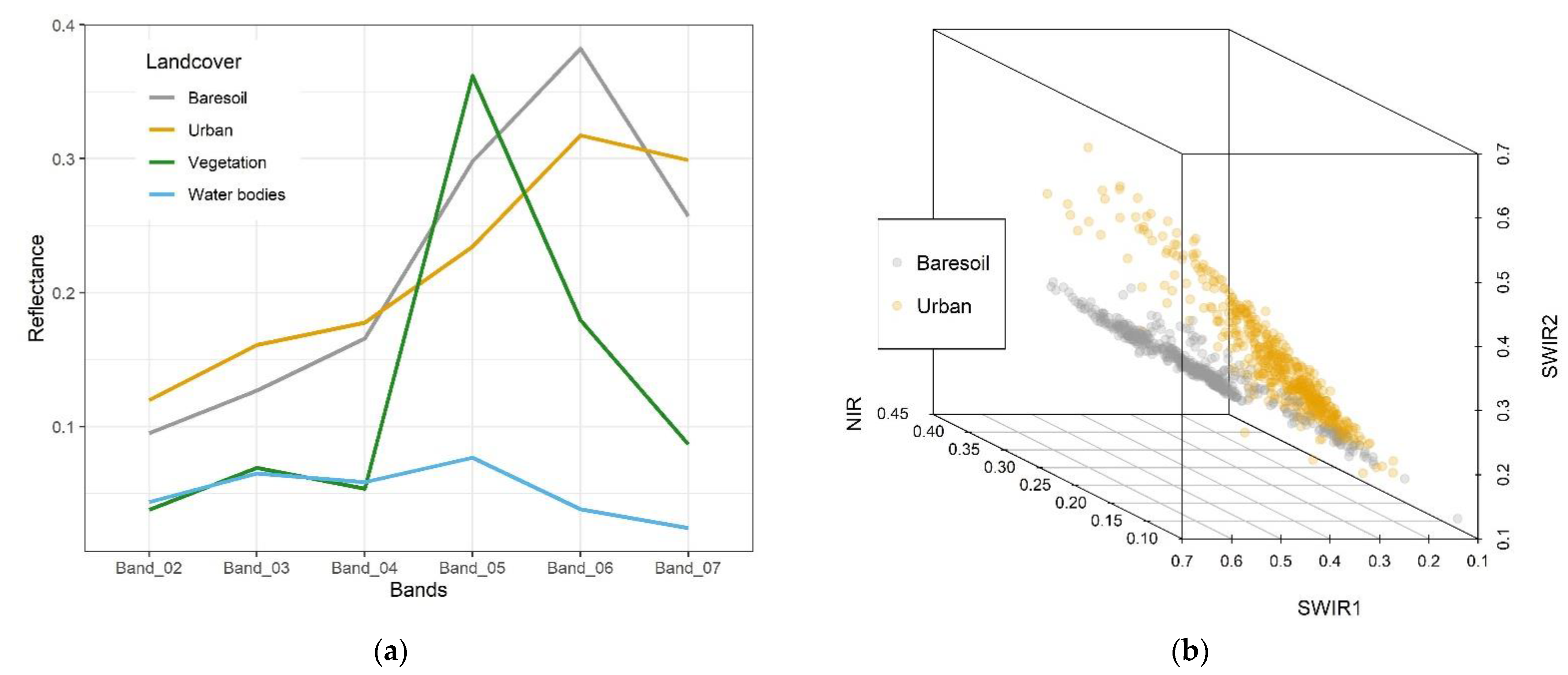
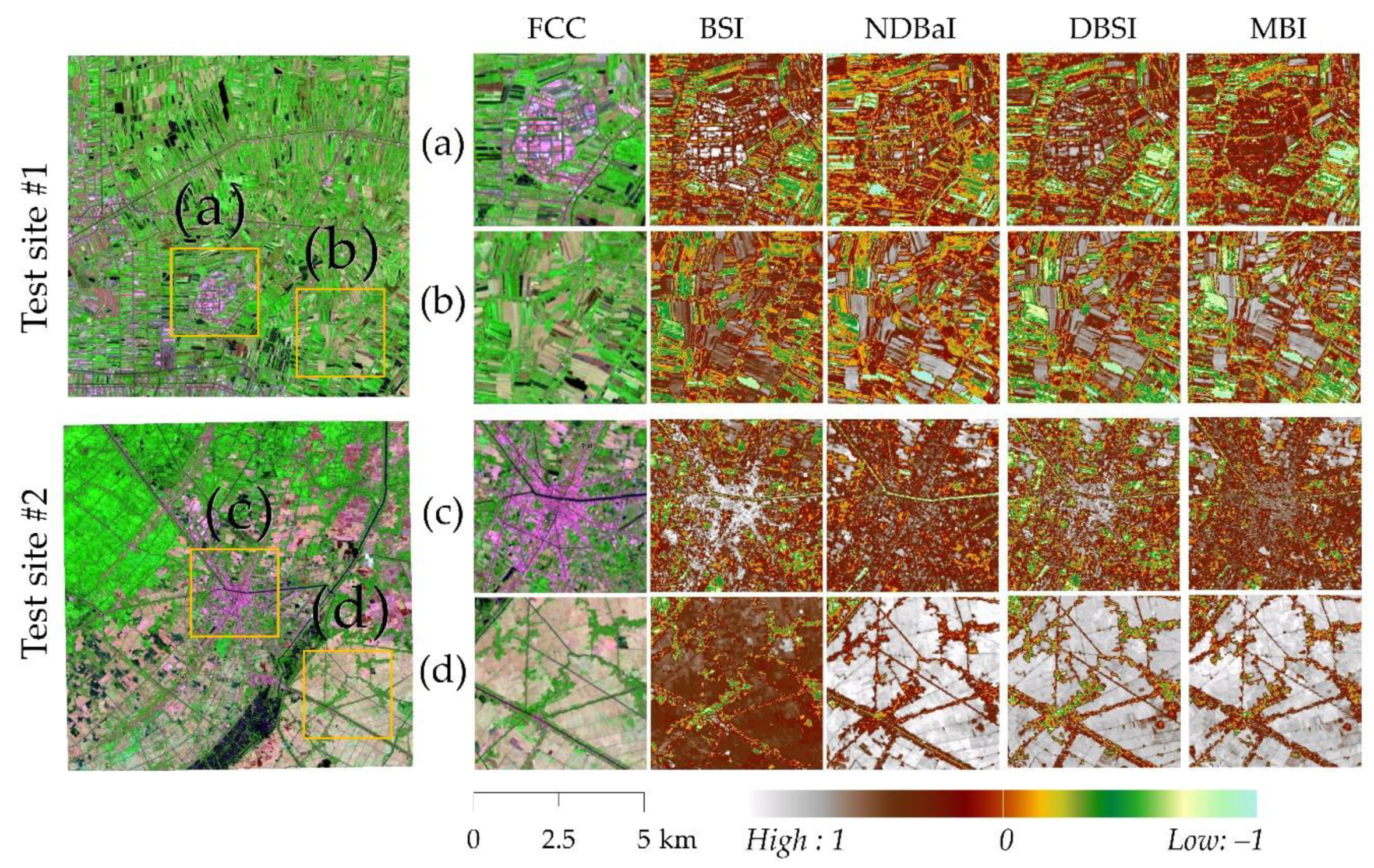
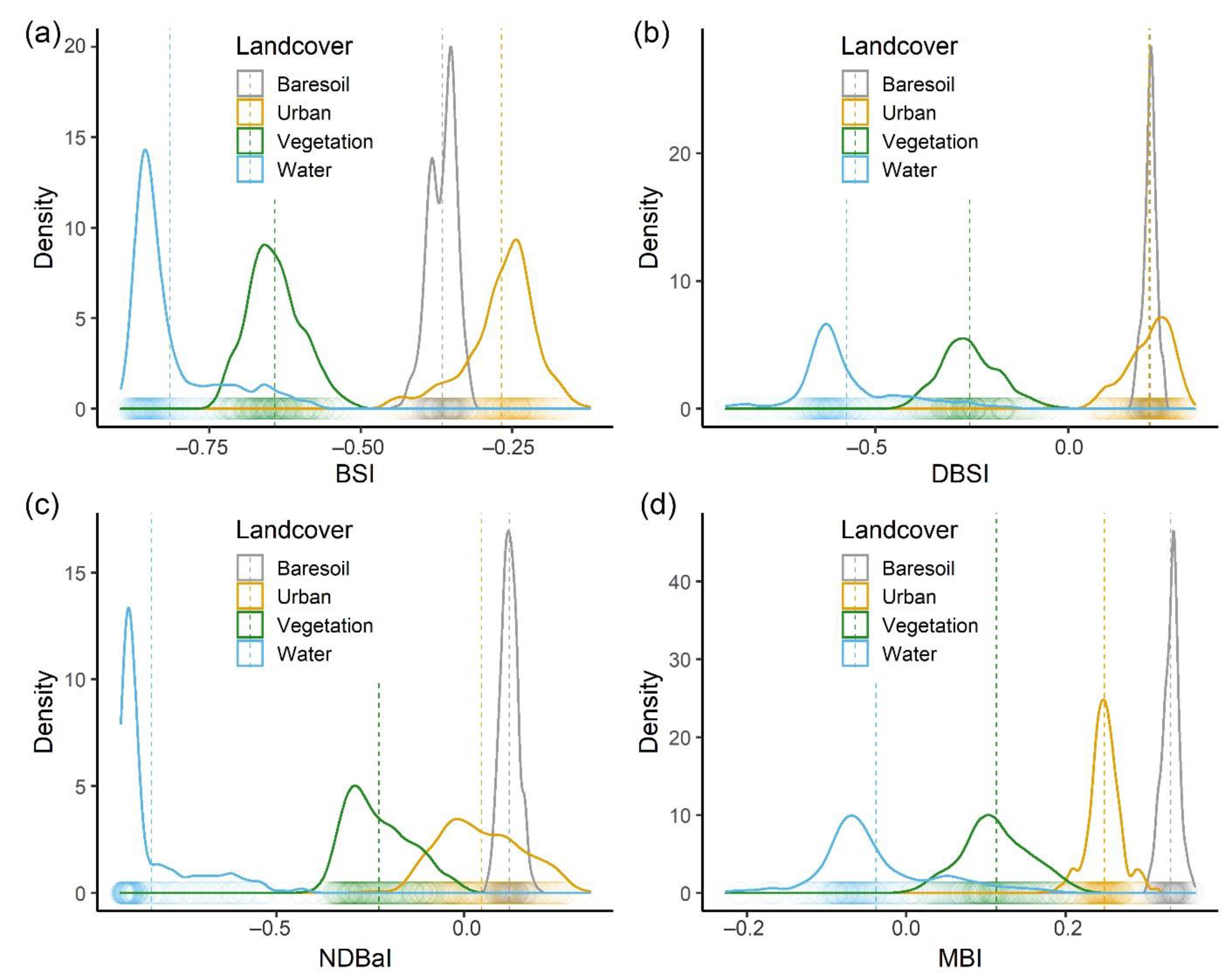
3.1. Bare Soil Indices

Four bare soil indices calculated for test sites #1 and #2 are presented in Figure 5. The index images were uniformly rescaled on a value range of −1 to 1 for peer comparison among the indices. Regarding image visibility, we can see that BSI emphasizes built-up covers instead of bare soil areas because buildings in index images are in a lighter tone (i.e., higher than 0.5) compared to bare soil parcels (Figure 5a,c). Although DBSI can better highlight bare areas against BSI, several built-up areas are still in a light tone, especially in the city center and buildings with high reflectance from roof materials. The NDBaI and our bare soil index, MBI, performed well for both bare soil emphasis and separation with built-up covers. Those bareness areas are able to be visibly identified by pixels with values moving towards 1.0 on both NDBaI and MBI (Figure 5b,d).

Density graphs were created by extracted points (i.e., 4000 points for both test sites), illustrating how land cover types are differently classified in BSI, NDBaI, DBSI, and MBI (Figure 6). The mean values of bare soil and urban areas in NDBaI and DBSI are overlaid (i.e., ${\overline{NDBaI}}_{baresoil}=0.122\pm 0.023$, ${\overline{NDBaI}}_{urban}=0.047\pm 0.110$ and ${\overline{DBSI}}_{baresoil}=0.212\pm 0.016$, ${\overline{DBSI}}_{urban}=0.209\pm 0.060$). An overlapping rate test shows the overlapping rate (OLR) between bare soil and urban pixels reaches 35% and 25% for DBSI and NDBaI, respectively. Therefore, determining an optimal thresholding value to differentiate bareness from urban areas is relatively challenging. Nevertheless, once we can pick out an approximate value, it does not mean that these two covers can be altogether distinguished because of existing overlapping. The mean ranges in BSI are relatively distinct, ${\overline{BSI}}_{baresoil}=-0.365\pm 0.022$ versus ${\overline{BSI}}_{urban}=-0.268\pm 0.058$, with the OLR at approximately 21%. There is another complication when using BSI for bare soil detection. BSI emphasizes urban features instead of bareness, so the most positive values on this index represent built-up areas. Therefore, the determination of the bare soil thresholding value in BSI is a double task with upper and lower limit values. MBI shows its efficiency with seemingly no overlapping zones for bare soil, built-up, and other land covers (Figure 6d). The MBI mean values for bare soil and urban features are $\overline{MBI}=0.332\pm 0.010$ and $\overline{MBI}=0.249\pm 0.020$, respectively. The OLR between bare soil and urban pixels does not exceed 10% on either test site. It reasonably implies the applicability of MBI in urban and bare soil discrimination.

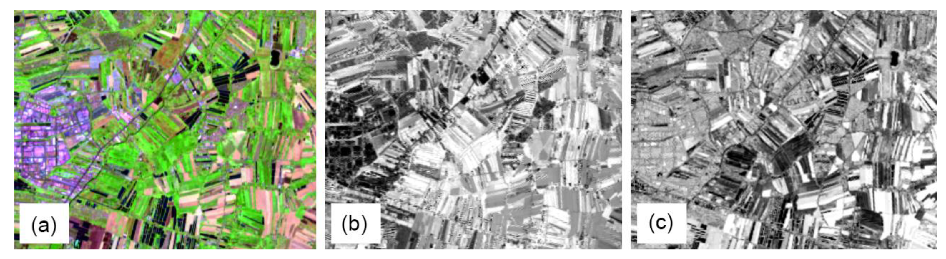
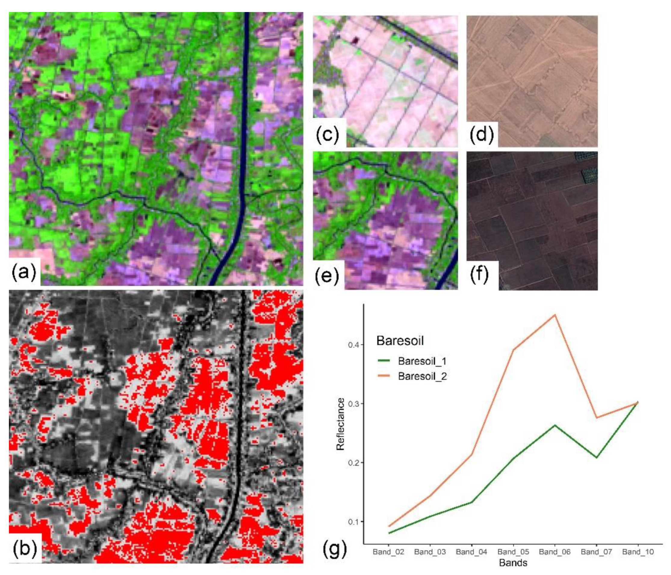
3.2. Extraction of Bare Soil Areas Using Modified Bare Soil Index

Bare soil index images were applied with different thresholding values for mapping ratio images into bare soil and other land cover types (i.e., as values out of the thresholding ranges). In the first test site, bare soil thresholding ranges were BSI $\left(-0.46 \mathrm{to} -0.32\right)$, NDBaI $\left(>0.0\right)$, DBSI $\left(>0.125\right)$, and MBI $\left(>0.27\right)$. The values were modified a little for the second test site due to its unique weather, soil, and land cover patterns, which were NDBaI $\left(>-0.05\right)$ and DBSI $\left(>0.10\right)$. The thresholding range was selected using MOT and a visualization technique based on image interpretation keys (e.g., color, tone, texture, size, shape, and association) when as much bare soil as possible is able to be retrieved.

The bare soil extraction results using threshold values are shown in Figure 7. Generally, these four indices were able to detect bare soil features, especially for large and homogeneous areas of bare soil (Figure 7b,c). Yet, the classification ability of these bareness indices is dissimilar. The BSI classified more bare soil areas than there are in reality, i.e., it is clearly depicted in the overview bare soil layers. For instance, once many bare soil areas were detected using the BSI index, several built-up areas were misclassified as bare soil (Figure 7a,c: BSI). The misclassification of bare soil was reduced when using the DBSI, but there are still buildings classified as having bare soil features, especially in the city core of Soc Trang province (test site #2) and a dense cluster of residential areas in eastern Bangkok (Figure 7a,c: DBSI). The extracted bareness layers using NDBaI and MBI were relatively similar to visible bare soil in composite images in terms of spatial patterns and distribution, except for some small-size and scattered residential areas that were incorrectly identified. The difference can only be seen in Figure 7a,c for NDBaI and MBI, where a strip of scattered residential areas and the city center were accurately classified as other land cover types by MBI instead of bare soil features as classified by NDBaI. In short, among four indices of bare soil, MBI is the most effective index in identifying bare soil features using index values in terms of visibility. Detection performance is detailed in Section 3.3.

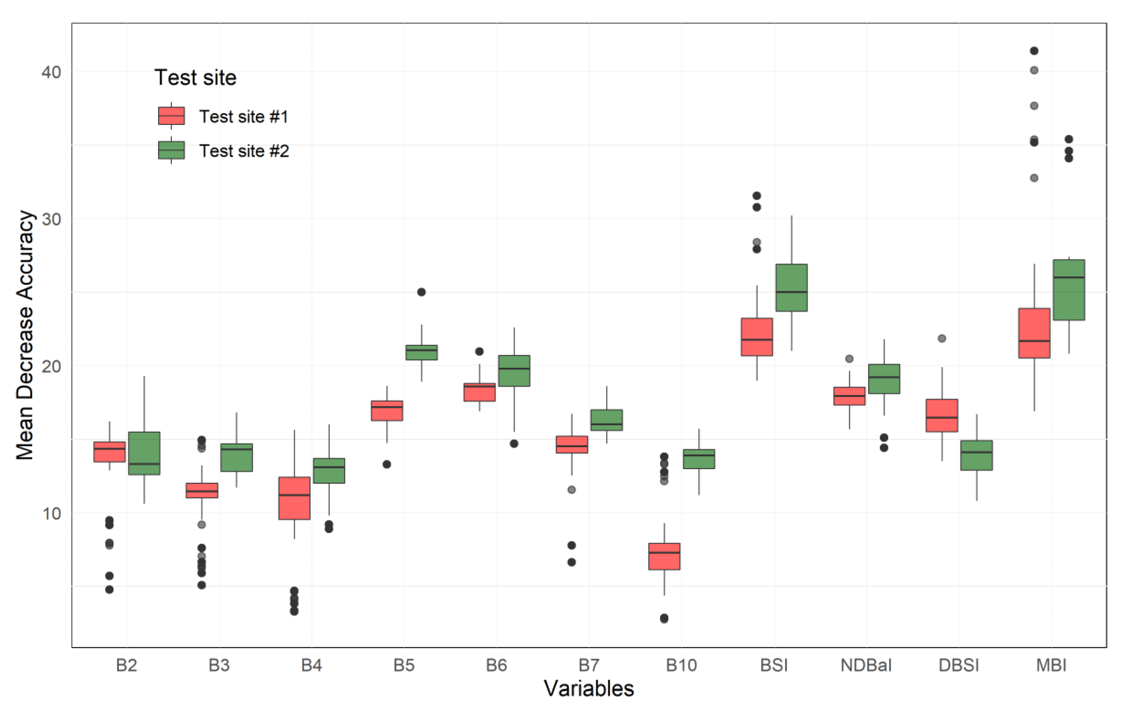
3.3. Performance Assessment

The bare soil layers were compared to ground truth points (i.e., the second dataset of pure pixels). The results were mainly evaluated by the overall accuracy and kappa coefficients (

Table 2. Accuracy assessment of bare soil features extracted by four bareness indices.

Site	Indicator	BSI	NDBaI	DBSI	MBI
Site #1	Overall Accuracy	93.2	96.5	91.0	98.0
	Kappa coefficient	0.87	0.93	0.82	0.96
Site #2	Overall Accuracy	84.3	92.8	91.5	98.5
	Kappa coefficient	0.72	0.86	0.83	0.97

). The DBSI and BSI did not perform well compared to other indices for classifying bareness in test site #1 $\left(K=0.82\right)$ and test site #2 $\left(K=0.72\right)$, respectively. The NDBaI was the second highest-performance index in detecting bare soil in test site #1 $\left(K=0.93\right)$ and test site #2 $\left(K=0.86\right)$. The new bareness index, MBI, effectively distinguished the bare soil from other urban covers. The kappa coefficients attained a level greater than 0.95 for both test sites for MBI. This assessment demonstrated the ability of MBI to detect bare soil regardless of bare soil patterns being sizeable or heterogeneous bare soil.

Figure 8 shows the important variable assessment using the RFC that reveals the MDA in test site #1 which is generally lower than the value in test site #2. The more extensive the bare soil areas are, the more misclassification there is liable to be. MBI is the most significant contributor to the classifier in comparison to the multispectral bands and three bare soil indices. The classification accuracy decreases by 28 ± 14.6% in test site #1 and 26.3 ± 4.2% in test site #2 without MBI. In test site #2, the accuracy drops by 77.1% without the contribution of MBI. The contribution of BSI is noticeable with the MDA about 22.7 ± 3.3% and 25.1 ± 2.3% in test sites #1 and #2, respectively. It is followed by the NDBaI with a small difference in MDA between the two test sites. The DBSI efficiency is relatively low in this test when its MDA lies between 14 ± 1.5% (test site #2) and 16.6 ± 1.3% (test site #1). Among the individual spectral bands, the TIR wavelength is indicated as the least contributing variable for the classification.

In contrast, it is predictable that NIR, SWIR1, and SWIR2 are the most individually meaningful contributors among the multispectral wavelengths. The contribution of these bands is even higher than that of NDBaI and DBSI. Once again, it demonstrates the rationale for suggesting band combination is appropriate, and the MBI has potentially higher efficiency than other indices in this study.

4. Discussions

Several remote sensing indices are derived from different spectral wavelengths to enhance and separate bare soil from other land cover features. Unlike some other indices (e.g., NDVI and MNDWI), which can be widely applied in many regions regardless of climate conditions and geographical features, the bare soil index is a relatively sensitive indicator. The bare soil index’s performance depends on soil composition, soil moisture, and even surrounding green covers [49,64]. Rasul [49] also indicated that the bare soil index’s performance differs in humid and dry-arid regions. For example, the dry bareness index (DBSI) was assessed as having high accuracy in Erbil (Iraq), but it is an inappropriate indicator for bareness mapping in our test sites (i.e., tropical monsoon regions). We should consider the study area’s climatic conditions as well as the effectiveness when choosing an appropriate bare soil index. Furthermore, surface characteristics should be considered when applying the spectral indices in general and the MBI in particular. For instance, the effectiveness of NDVI in vegetation detection is negatively influenced by urban architectures such as cool roofs, cool pavement materials, and rooftop gardens. Similarly, the MBI performance may be affected by urban materials such as clay roof tiles and road paving bricks.

The modified bare soil index (MBI) is based on NIR, SWIR1, and SWIR2 spectral wavelengths. This index shows the ability to effectively distinguish bare soil from other areas at both test sites. Meanwhile, the NDBaI also had high isolation efficiency (Table 2), but the accuracies varied between these two test sites. Thus, we can primarily consider that bare soil classification efficiency by the applied MBI is independent of bare soil and urban patterns. Compared with the NDBaI, the proposed index utilizes infrared wavelengths with similar pixel resolution instead of the 100 m thermal infrared band in Landsat 8.

Additionally, the application of NDBaI for finer resolution satellites, e.g., Sentinel-2, WorldView, is impossible because the thermal infrared band is unavailable from these satellites. However, the wavelengths required for MBI estimation are all applicable for Sentinel-2 and WorldView. MBI can even be considered for bare soil-related studies at larger scales using low-resolution data such as MODIS and Sentinel-3. Therefore, the MBI may provide a better option and has the potential to be applied to a wide range of data in bare soil-related research, such as the pre-urbanization stage and agricultural losses caused by natural disasters. Although there are comparable spectrum bands among the satellites, the dissimilarities in pixel size and central wavelengths may affect the MBI’s performance. Therefore, empirical studies on MBI’s ability to identify bare soil based on the data mentioned earlier are expected to be carried out in the future.

There are two kinds of bare soil which are visible in a color composite image, namely dry and humid bare soil (Figure 9c–f). The dry bare soil (type #2) has a high reflectance value in shortwave infrared wavelengths, while humid bare soil (type#1) has a low reflectance value in these wavelengths, absorbed by high moisture content (Figure 9g). Therefore, the humid bare soil is identified as urban features (Figure 9a,b). When we reduce the MBI thresholding value to select the whole area of humid bare soil, several urban areas are misclassified. Fortunately, the humid bare soil is uncommon in both test sites, so it does not significantly affect the general bare soil extraction. Despite this, future studies should continue to seek an index or technique to complete the distinction between urban areas and wet bare soil for research in urban, semi-urban, and countryside areas.

5. Conclusions

We enhanced the bare soil signals by a three-band bare soil index called modified bare soil index (MBI) using NIR, SWIR1, and SWIR2 wavelengths in Landsat 8 to precisely classify and differentiate bare soil from built-up and other land covers, especially for areas disturbed by seasonal bare soil in the tropical regions. The value range of urban area and bareness in MBI has fewer overlapping zones in comparison to BSI, NDBaI, and DBSI, whereby MBI significantly reduces misclassification between built-up and bare soil features. Bare soil areas derived by MBI thresholding value achieved high accuracy with kappa coefficients over 0.96 and overall accuracy higher than 98% in the study areas. The MBI is also a critical predictor in land cover classification compared to individual bands and other considered bare soil indices.

The proposed MBI is a potential option for classifying bare soil in the tropical climatic region. Usage of MBI is more efficient than NDBaI, which is based on a low resolution thermal infrared wavelength in Landsat 8. Besides, the MBI might be applicable for a finer satellite such as Sentinel 2, WorldView, and any satellite with similar spectrum bands. Yet, when applying MBI, climatic conditions, bare soil patterns, and land cover characteristics should be considered to optimize the bare soil index’s effectiveness.

References

1. Dou, P.; Chen, Y. Dynamic monitoring of land-use/land-cover change and urban expansion in shenzhen using landsat imagery from 1988 to 2015. Int. J. Remote Sens. 2017, 38, 5388–5407. [Google Scholar] [CrossRef]
2. Zhang, Y.; Shen, W.; Li, M.; Lv, Y. Assessing spatio-temporal changes in forest cover and fragmentation under urban expansion in Nanjing, eastern China, from long-term Landsat observations (1987–2017). Appl. Geogr. 2020, 117, 102190. [Google Scholar] [CrossRef]
3. Chai, B.; Li, P. Annual Urban Expansion Extraction and Spatio-Temporal Analysis Using Landsat Time Series Data: A Case Study of Tianjin. IEEE J. Sel. Top. Appl. Earth Obs. Remote Sens. 2018, 11, 2644–2656. [Google Scholar] [CrossRef]
4. Schultz, M.; Clevers, J.G.P.W.; Carter, S.; Verbesselt, J.; Avitabile, V.; Quang, H.V.; Herold, M. Performance of vegetation indices from Landsat time series in deforestation monitoring. Int. J. Appl. Earth Obs. Geoinf. 2016, 52, 318–327. [Google Scholar] [CrossRef]
5. Hamunyela, E.; Verbesselt, J.; Herold, M. Using spatial context to improve early detection of deforestation from Landsat time series. Remote Sens. Environ. 2016, 172, 126–138. [Google Scholar] [CrossRef]
6. Souza, C.M.; Siqueira, J.V.; Sales, M.H.; Fonseca, A.V.; Ribeiro, J.G.; Numata, I.; Cochrane, M.A.; Barber, C.P.; Roberts, D.A.; Barlow, J. Ten-year landsat classification of deforestation and forest degradation in the brazilian amazon. Remote Sens. 2013, 5, 5493–5513. [Google Scholar] [CrossRef] [Green Version]
7. Zhu, F.; Wang, H.; Li, M.; Diao, J.; Shen, W.; Zhang, Y.; Wu, H. Characterizing the effects of climate change on short-term post-disturbance forest recovery in southern China from Landsat time-series observations (1988–2016). Front. Earth Sci. 2020, 14, 816–827. [Google Scholar] [CrossRef]
8. Mo, Y.; Kearney, M.S.; Turner, R.E. Feedback of coastal marshes to climate change: Long-term phenological shifts. Ecol. Evol. 2019, 9, 6785–6797. [Google Scholar] [CrossRef] [Green Version]
9. Hislop, S.; Jones, S.; Soto-Berelov, M.; Skidmore, A.; Haywood, A.; Nguyen, T.H. Using landsat spectral indices in time-series to assess wildfire disturbance and recovery. Remote Sens. 2018, 10, 460. [Google Scholar] [CrossRef] [Green Version]
10. Meddens, A.J.H.; Kolden, C.A.; Lutz, J.A. Detecting unburned areas within wildfire perimeters using Landsat and ancillary data across the northwestern United States. Remote Sens. Environ. 2016, 186, 275–285. [Google Scholar] [CrossRef]
11. Jilge, M.; Heiden, U.; Neumann, C.; Feilhauer, H. Gradients in urban material composition: A new concept to map cities with spaceborne imaging spectroscopy data. Remote Sens. Environ. 2019, 223, 179–193. [Google Scholar] [CrossRef]
12. Hamedianfar, A.; Shafri, H.Z.M. Integrated approach using data mining-based decision tree and object-based image analysis for high-resolution urban mapping of WorldView-2 satellite sensor data. J. Appl. Remote Sens. 2016, 10, 025001. [Google Scholar] [CrossRef]
13. Sertel, E.; Akay, S.S. High resolution mapping of urban areas using SPOT-5 images and ancillary data. Int. J. Environ. Geoinformatics 2015, 2, 63–76. [Google Scholar] [CrossRef] [Green Version]
14. Deng, J.; Huang, Y.; Chen, B.; Tong, C.; Liu, P.; Wang, H.; Hong, Y. A methodology to monitor urban expansion and green space change using a time series of multi-sensor SPOT and Sentinel-2A images. Remote Sens. 2019, 11, 1230. [Google Scholar] [CrossRef] [Green Version]
15. Qiu, C.; Schmitt, M.; Geiß, C.; Chen, T.H.K.; Zhu, X.X. A framework for large-scale mapping of human settlement extent from Sentinel-2 images via fully convolutional neural networks. ISPRS J. Photogramm. Remote Sens. 2020, 163, 152–170. [Google Scholar] [CrossRef] [PubMed]
16. Song, Y.; Chen, B.; Kwan, M.P. How does urban expansion impact people’s exposure to green environments? A comparative study of 290 Chinese cities. J. Clean. Prod. 2020, 246, 119018. [Google Scholar] [CrossRef]
17. Iannelli, G.C.; Gamba, P. Jointly exploiting Sentinel-1 and Sentinel-2 for urban mapping. IEEE Int. Geosci. Remote Sens. Symp. 2018, 8209–8212. [Google Scholar] [CrossRef]
18. Tavares, P.A.; Beltrão, N.E.S.; Guimarães, U.S.; Teodoro, A.C. Integration of sentinel-1 and sentinel-2 for classification and LULC mapping in the urban area of Belém, eastern Brazilian Amazon. Sensors 2019, 19, 1140. [Google Scholar] [CrossRef] [Green Version]
19. Wulder, M.A.; Loveland, T.R.; Roy, D.P.; Crawford, C.J.; Masek, J.G.; Woodcock, C.E.; Allen, R.G.; Anderson, M.C.; Belward, A.S.; Cohen, W.B.; et al. Current status of Landsat program, science, and applications. Remote Sens. Environ. 2019, 225, 127–147. [Google Scholar] [CrossRef]
20. Shiflett, S.A.; Liang, L.L.; Crum, S.M.; Feyisa, G.L.; Wang, J.; Jenerette, G.D. Variation in the urban vegetation, surface temperature, air temperature nexus. Sci. Total Environ. 2017, 579, 495–505. [Google Scholar] [CrossRef]
21. Voogt, J.A.; Oke, T.R. Thermal remote sensing of urban climates. Remote Sens. Environ. 2003, 86, 370–384. [Google Scholar] [CrossRef]
22. Estoque, R.C.; Murayama, Y. Monitoring surface urban heat island formation in a tropical mountain city using Landsat data (1987–2015). ISPRS J. Photogramm. Remote Sens. 2017, 133, 18–29. [Google Scholar] [CrossRef]
23. Nurwanda, A.; Honjo, T. The Prediction of City Expansion and Land Surface Temperature in Bogor City, Indonesia. Sustain. Cities Soc. 2019, 52, 101772. [Google Scholar] [CrossRef]
24. Son, N.T.; Chen, C.F.; Chen, C.R. Urban expansion and its impacts on local temperature in San Salvador, El Salvador. Urban Clim. 2020, 32, 100617. [Google Scholar] [CrossRef]
25. Gamba, P.; Acqua, F.D. Increased accuracy multiband urban classification using a neuro-fuzzy classifier. Int. J. Remote Sens. 2003, 24, 827–834. [Google Scholar] [CrossRef]
26. Marconcini, M.; Metz-Marconcini, A.; Üreyen, S.; Palacios-Lopez, D.; Hanke, W.; Bachofer, F.; Zeidler, J.; Esch, T.; Gorelick, N.; Kakarla, A.; et al. Outlining where humans live, the World Settlement Footprint 2015. Sci. Data 2020, 7, 1–14. [Google Scholar] [CrossRef]
27. Pesaresi, M.; Ehrlich, D.; Ferri, S.; Florczyk, A.J.; Freire, S.; Halkia, M.; Julea, A.; Kemper, T.; Soille, P.; Syrris, V. Operating Procedure for the Production of the Global Human Settlement Layer from Landsat Data of the Epochs 1975, 1990, 2000, and 2014; Publications Office of the European Union: Luxembourg, 2016. [Google Scholar]
28. Pesaresi, M.; Huadong, G.; Blaes, X.; Ehrlich, D.; Ferri, S.; Gueguen, L.; Halkia, M.; Kauffmann, M.; Kemper, T.; Lu, L.; et al. A global human settlement layer from optical HR/VHR RS data: Concept and first results. IEEE J. Sel. Top. Appl. Earth Obs. Remote Sens. 2013, 6, 2102–2131. [Google Scholar] [CrossRef]
29. Kuenzer, C.; Guo, H.; Huth, J.; Leinenkugel, P.; Li, X.; Dech, S. Flood mapping and flood dynamics of the mekong delta: ENVISAT-ASAR-WSM based time series analyses. Remote Sens. 2013, 5, 687–715. [Google Scholar] [CrossRef] [Green Version]
30. Leinenkugel, P.; Kuenzer, C.; Dech, S. Comparison and enhancement of MODIS cloud mask products for Southeast Asia. Int. J. Remote Sens. 2013, 34, 2730–2748. [Google Scholar] [CrossRef]
31. As-syakur, A.R.; Adnyana, I.W.S.; Arthana, I.W.; Nuarsa, I.W. Enhanced built-Up and bareness index (EBBI) for mapping built-up and bare land in an urban area. Remote Sens. 2012, 4, 2957–2970. [Google Scholar] [CrossRef] [Green Version]
32. Li, S.; Chen, X. A new bare-soil index for rapid mapping developing areas using landsat 8 data. Int. Arch. Photogramm. Remote Sens. Spat. Inf. Sci. ISPRS Arch. 2014, 40, 139–144. [Google Scholar] [CrossRef] [Green Version]
33. Engelstaedter, S.; Kohfeld, K.E.; Tegen, I.; Harrison, S.P. Controls of dust emissions by vegetation and topographic depressions: An evaluation using dust storm frequency data. Geophys. Res. Lett. 2003, 30, 30–33. [Google Scholar] [CrossRef]
34. Chen, W.; Liu, L.; Zhang, C.; Wang, J.; Wang, J.; Pan, Y. Monitoring the seasonal bare soil areas in Beijing using multi-temporal TM images. Int. Geosci. Remote Sens. Symp. 2004, 5, 3379–3382. [Google Scholar] [CrossRef]
35. Eroǧlu, H.; Çakir, G.; Sivrikaya, F.; Akay, A.E. Using high resolution images and elevation data in classifying erosion risks of bare soil areas in the Hatila Valley Natural Protected Area, Turkey. Stoch. Environ. Res. Risk Assess. 2010, 24, 699–704. [Google Scholar] [CrossRef]
36. Tayfur, G.; Ozdemir, S.; Singh, V.P. Fuzzy logic algorithm for runoff-induced sediment transport from bare soil surfaces. Adv. Water Resour. 2003, 26, 1249–1256. [Google Scholar] [CrossRef] [Green Version]
37. Labrière, N.; Locatelli, B.; Laumonier, Y.; Freycon, V.; Bernoux, M. Soil erosion in the humid tropics: A systematic quantitative review. Agric. Ecosyst. Environ. 2015, 203, 127–139. [Google Scholar] [CrossRef]
38. Carlan, I.; Haase, D.; Große-Stoltenberg, A.; Sandric, I. Mapping heat and traffic stress of urban park vegetation based on satellite imagery-A comparison of Bucharest, Romania and Leipzig, Germany. Urban Ecosyst. 2020, 23, 363–377. [Google Scholar] [CrossRef]
39. Nguyen, A.N. Historic drought and salinity intrusion in the Mekong Delta in 2016: Lessons learned and response solutions. Vietnam J. Sci. Technol. Eng. 2017, 59, 93–96. [Google Scholar] [CrossRef]
40. Diep, N.T.H.; Korsem, T.; Can, N.T.; Phonphan, W. Vo Quang Minh Determination of aquaculture distribution by using remote sensing technology in Thanh Phu district, Ben Tre province, Vietnam. Vietnam, J. Sci. Technol. Eng. 2019, 61, 35–41. [Google Scholar] [CrossRef] [Green Version]
41. Van Thao, N.; Cu, N.D.; Thanh, N.X. Maping and detecting fallowed area of cultivated tiger shrimp ponds of coastal provinces by using remote sensing data. J. Mar. Sci. Technol. 2012, 12, 34–45. [Google Scholar] [CrossRef]
42. Koroleva, P.V.; Rukhovich, D.I.; Rukhovich, A.D.; Rukhovich, D.D.; Kulyanitsa, A.L.; Trubnikov, A.V.; Kalinina, N.V.; Simakova, M.S. Location of Bare Soil Surface and Soil Line on the RED–NIR Spectral Plane. Eurasian Soil Sci. 2017, 50, 1375–1385. [Google Scholar] [CrossRef]
43. Koroleva, P.V.; Rukhovich, D.I.; Rukhovich, A.D.; Rukhovich, D.D.; Kulyanitsa, A.L.; Trubnikov, A.V.; Kalinina, N.V.; Simakova, M.S. Characterization of Soil Types and Subtypes in N-Dimensional Space of Multitemporal (Empirical) Soil Line. Eurasian Soil Sci. 2018, 51, 1021–1033. [Google Scholar] [CrossRef]
44. Lin, H.; Wang, J.; Liu, S.; Qu, Y.; Wan, H. Studies on urban areas extraction from Landsat TM images. Int. Geosci. Remote Sens. Symp. 2005, 6, 3826–3829. [Google Scholar] [CrossRef]
45. Jamalabd, M.S.; Abkar, A.A. Forest Canopy Density Monitoring, Using Satellite Images. In Proceedings of the International Society for Photogrammetry and Remote Sensing (ISPRS); ISPRS Congress: Istanbul, Turkey, 2004; pp. 12–23. [Google Scholar]
46. Rogers, A.S.; Kearney, M.S. Reducing signature variability in unmixing coastal marsh Thematic Mapper scenes using spectral indices. Int. J. Remote Sens. 2004, 25, 2317–2335. [Google Scholar] [CrossRef]
47. Wentzel, K. Determination of the overall soil erosion potential in the nsikazi district (mpumalanga province, south africa) using remote sensing and GIS. Can. J. Remote Sens. 2002, 28, 322–327. [Google Scholar] [CrossRef]
48. Diek, S.; Fornallaz, F.; Schaepman, M.E.; de Jong, R. Barest Pixel Composite for agricultural areas using landsat time series. Remote Sens. 2017, 9, 1245. [Google Scholar] [CrossRef] [Green Version]
49. Rasul, A.; Balzter, H.; Ibrahim, G.R.F.; Hameed, H.M.; Wheeler, J.; Adamu, B.; Ibrahim, S.; Najmaddin, P.M. Applying built-up and bare-soil indices from Landsat 8 to cities in dry climates. Land 2018, 7, 81. [Google Scholar] [CrossRef] [Green Version]
50. Deng, Y.; Wu, C.; Li, M.; Chen, R. RNDSI: A ratio normalized difference soil index for remote sensing of urban/suburban environments. Int. J. Appl. Earth Obs. Geoinf. 2015, 39, 40–48. [Google Scholar] [CrossRef]
51. Xu, H. Modification of normalised difference water index (NDWI) to enhance open water features in remotely sensed imagery. Int. J. Remote Sens. 2006, 27, 3025–3033. [Google Scholar] [CrossRef]
52. Zhao, H.; Chen, X. Use of normalized difference bareness index in quickly mapping bare areas from TM/ETM+. Int. Geosci. Remote Sens. Symp. 2005, 3, 1666–1668. [Google Scholar] [CrossRef]
53. Li, H.; Wang, C.; Zhong, C.; Su, A.; Xiong, C.; Wang, J.; Liu, J. Mapping urban bare land automatically from Landsat imagery with a simple index. Remote Sens. 2017, 9, 700. [Google Scholar] [CrossRef] [Green Version]
54. Piyoosh, A.K.; Ghosh, S.K. Development of a modified bare soil and urban index for Landsat 8 satellite data. Geocarto Int. 2018, 33, 423–442. [Google Scholar] [CrossRef]
55. Adulkongkaew, T.; Satapanajaru, T.; Charoenhirunyingyos, S. Effects of Agricultural Suburb on Urban Heat Island of Bangkok Metropolitan City, Thailand. In Proceedings of the 5th International Conference on Chemical, Agricultural, Biological and Environmental Sciences, Kyoto, Japan, 18–19 April 2017; pp. 42–49. [Google Scholar]
56. Jongkroy, P. Urbanization and changing settlement patterns in Peri-urban Bangkok. Kasetsart J. Soc. Sci. 2009, 30, 303–312. [Google Scholar]
57. Nguyen, D.B.; Clauss, K.; Cao, S.; Naeimi, V.; Kuenzer, C.; Wagner, W. Mapping Rice Seasonality in the Mekong Delta with multi-year envisat ASAR WSM Data. Remote Sens. 2015, 7, 15868–15893. [Google Scholar] [CrossRef] [Green Version]
58. DLD Comparison of Thailand’s Soil Classification and the World Reference Base (WRB); Department of Land Development: Bangkok, Thailand, 2011.
59. Nguyen, P.M.; Van Le, K.; Botula, Y.D.; Cornelis, W.M. Evaluation of soil water retention pedotransfer functions for Vietnamese Mekong Delta soils. Agric. Water Manag. 2015, 158, 126–138. [Google Scholar] [CrossRef]
60. Equere, V.; Mirzaei, P.A.; Riffat, S. Definition of a new morphological parameter to improve prediction of urban heat island. Sustain. Cities Soc. 2020, 56, 102021. [Google Scholar] [CrossRef]
61. Yan, W.Y.; Shaker, A.; El-Ashmawy, N. Urban land cover classification using airborne LiDAR data: A review. Remote Sens. Environ. 2015, 158, 295–310. [Google Scholar] [CrossRef]
62. Panda, S.S.; Masson, E.; Sen, S.; Kim, H.W.; Amatya, D.M. Geospatial technology applications in forest hydrology. In Forest hydrology: Processes, Management and Assessment; CABI: Wallingford, UK, 2016; pp. 162–179. [Google Scholar]
63. Kartika, T.; Arifin, S.; Sari, I.L.; Tosiani, A.; Firmansyah, R.; Kustiyo; Carolita, I.; Adi, K.; Daryanto, A.F.; Said, Z. Analysis of Vegetation Indices Using Metric Landsat-8 Data to Identify Tree Cover Change in Riau Province. IOP Conf. Ser. Earth Environ. Sci. 2019, 280. [Google Scholar] [CrossRef]
64. Yue, J.; Tian, J.; Tian, Q.; Xu, K.; Xu, N. Development of soil moisture indices from differences in water absorption between shortwave-infrared bands. ISPRS J. Photogramm. Remote Sens. 2019, 154, 216–230. [Google Scholar] [CrossRef]
65. Rikimaru, A.; Roy, P.S.; Miyatake, S. Tropical forest cover density mapping. Trop. Ecol. 2002, 43, 39–47. [Google Scholar]
66. Mostofi, N.; Hasanlou, M. Feature selection of various land cover indices for monitoring surface heat island in Tehran city using Landsat 8 imagery. J. Environ. Eng. Landsc. Manag. 2017, 25, 241–250. [Google Scholar] [CrossRef] [Green Version]
67. Fernando, T.; Gunawardena, A. Determination of convertion of tea lands in Kandy District using different remote sensing indices. In Proceedings of the 37th Asian Conference on Remote Sensing, ACRS 2016, Colombo, Sri Lanka, 17–21 October 2016; Volume 1, pp. 161–166. [Google Scholar]
68. Sun, Q.; Wu, Z.; Tan, J. The relationship between land surface temperature and land use/land cover in Guangzhou, China. Environ. Earth Sci. 2012, 65, 1687–1694. [Google Scholar] [CrossRef]
69. Fan, F.; Fan, W.; Weng, Q. Improving Urban Impervious Surface Mapping by Linear Spectral Mixture Analysis and Using Spectral Indices. Can. J. Remote Sens. 2015, 41, 577–586. [Google Scholar] [CrossRef]
70. Hasanlou, M.; Mostofi, N. Investigating Urban Heat Island Effects and Relation Between Various Land Cover Indices in Tehran City Using Landsat 8 Imagery. In Proceedings of the 1st International Electronic Conference on Remote Sensing, Basel, Switzerland, 22 June–5 July 2015. [Google Scholar]
71. Diem, P.K.; Pimple, U.; Sitthi, A.; Varnakovida, P.; Tanaka, K.; Pungkul, S.; Leadprathom, K.; LeClerc, M.Y.; Chidthaisong, A. Shifts in growing season of tropical deciduous forests as driven by El Niño and La Niña during 2001–2016. Forests 2018, 9, 448. [Google Scholar] [CrossRef] [Green Version]
72. Mohd, O.; Suryanna, N.; Sahibuddin, S.S.; Abdollah, M.F. Thresholding and Fuzzy Rule-Based Classification Approaches in Handling Mangrove Forest Mixed Pixel Problems Associated with in QuickBird Remote Sensing Image Analysis. Int. J. Agric. For. 2012, 2, 300–306. [Google Scholar] [CrossRef] [Green Version]
73. Estoque, R.C.; Murayama, Y.; Myint, S.W. Effects of landscape composition and pattern on land surface temperature: An urban heat island study in the megacities of Southeast Asia. Sci. Total Environ. 2017, 577, 349–359. [Google Scholar] [CrossRef] [PubMed]
74. Du, Y.; Zhang, Y.; Ling, F.; Wang, Q.; Li, W.; Li, X. Water Bodies’ Mapping from Sentinel-2 Imagery with Modified Normalized Difference Water Index at 10-m Spatial Resolution Produced by Sharpening the SWIR Band. Remote Sens. 2016, 8, 354. [Google Scholar] [CrossRef] [Green Version]
75. Mzid, N.; Pignatti, S.; Huang, W.; Casa, R. An analysis of bare soil occurrence in arable croplands for remote sensing topsoil applications. Remote Sens. 2021, 13, 474. [Google Scholar] [CrossRef]
76. Qiu, B.; Zhang, K.; Tang, Z.; Chen, C.; Wang, Z. Developing soil indices based on brightness, darkness, and greenness to improve land surface mapping accuracy. GIScience Remote Sens. 2017, 54, 759–777. [Google Scholar] [CrossRef]
77. Nobuyuki Otsu A Threshold Selection Method from Gray-Level Histograms. IEEE Trans. Syst. Man Cybern 1979, 9, 62–66. [CrossRef] [Green Version]
78. Tran, D.X.; Pla, F.; Latorre-Carmona, P.; Myint, S.W.; Caetano, M.; Kieu, H.V. Characterizing the relationship between land use land cover change and land surface temperature. ISPRS J. Photogramm. Remote Sens. 2017, 124, 119–132. [Google Scholar] [CrossRef] [Green Version]
79. Rimal, B.; Zhang, L.; Keshtkar, H.; Wang, N.; Lin, Y. Monitoring and modeling of spatiotemporal urban expansion and land-use/land-cover change using integrated Markov chain cellular automata model. ISPRS Int. J. Geo Inf. 2017, 6, 288. [Google Scholar] [CrossRef] [Green Version]
80. Noi, P.T.; Kappas, M. Comparison of Random Forest, k-Nearest Neighbor, and Support Vector Machine Classifiers for Land Cover Classification Using Sentinel-2 Imagery. Sensors 2018, 18, 18. [Google Scholar] [CrossRef] [Green Version]
81. Olofsson, P.; Foody, G.M.; Herold, M.; Stehman, S.V.; Woodcock, C.E.; Wulder, M.A. Good practices for estimating area and assessing accuracy of land change. Remote Sens. Environ. 2014, 148, 42–57. [Google Scholar] [CrossRef]
82. Avashia, V.; Garg, A. Implications of land use transitions and climate change on local flooding in urban areas: An assessment of 42 Indian cities. Land Use Policy 2020, 95, 104571. [Google Scholar] [CrossRef]
83. Richards, J.A. Remote Sensing Digital Image Analysis; Springer: Berlin, Germany, 1999. [Google Scholar]
84. Jeffreys, H. An invariant form for the prior probability in estimation problems. In Proceedings of the Royal Society of London; Series A, Mathematical and Physical Sciences; Royal Society: London, UK, 1946; Volume 186, pp. 453–461. [Google Scholar]
85. Firozjaei, M.K.; Sedighi, A.; Kiavarz, M.; Qureshi, S.; Haase, D.; Alavipanah, S.K. Automated built-up extraction index: A new technique for mapping surface built-up areas using LANDSAT 8 OLI imagery. Remote Sens. 2019, 11, 1966. [Google Scholar] [CrossRef] [Green Version]
86. Pimple, U.; Sitthi, A.; Simonetti, D.; Pungkul, S.; Leadprathom, K.; Chidthaisong, A. Topographic correction of Landsat TM-5 and Landsat OLI-8 imagery to improve the performance of forest classification in the mountainous terrain of Northeast Thailand. Sustainability 2017, 9, 258. [Google Scholar] [CrossRef] [Green Version]
87. Han, H.; Guo, X.; Yu, H. Variable selection using Mean Decrease Accuracy and Mean Decrease Gini based on Random Forest. In Proceedings of the 2016 7th IEEE International Conference on Software Engineering and Service Science (ICSESS), Beijing, China, 26–28 August 2016; pp. 219–224. [Google Scholar] [CrossRef]
Figure 1. Flowchart showing the detailed research methodology to develop and validate the modified bare soil index.
Land 10 00231 g001
Figure 2. Map of the test sites in eastern Bangkok metropolis (test site #1) and central Soc Trang province (test size #2), false-color composite Landsat 8 (RGB: 7-5-3), pink and prune represent built-up and bare soil.
Land 10 00231 g002
Figure 3. (a) Spectral profiles show reflectance properties of different land cover types; (b) 3D plot presents spatial separation of bare soil and built-up samples based on reflectance values in NIR, SWIR1, and SWIR2 bands. Orange and gray dots represent bare soil and built-up samples, respectively.
Land 10 00231 g003
Figure 4. Magnified images (a) false-color composite (RGB: 7-5-3) with pink and prune representing built-up and bare soil, (b) normalized image on SWIR1 and SWIR2 (Equation (1)), which mostly highlights vegetation with bright tone, bare soil in gray and urban areas in black, and (c) three-band bare soil index (Equation (2)) emphasizing bare soil (bright tone), urban features in gray and vegetation in black.
Land 10 00231 g004
Figure 5. False-color composite (RGB: 7-5-3) on entire test sites and zoom-in regions in typical urban and bare land areas describing distinguishability between bare soil and other land cover types on different indices: (a,c) DBSI, (b,d) NDBaI and MBI.
Land 10 00231 g005
Figure 6. The density graph illustrates the density distribution of four land cover types for (a) bare soil index (BSI), (b) normalized difference bareness index (NDBaI), (c) dry bare-soil index (DBSI), and (d) modified bare soil index (MBI). Dash lines present mean values, and darker zones on horizontal show more concentrated data zones.
Land 10 00231 g006
Figure 7. Spatial distribution of bare soil layers extracted from BSI, NDBaI, DBSI, and MBI on entire test sites and zoom-in areas in solid line squares where there were significant differences among the indices compared to FCC images: (a,b) Test site #1, (c,d) Test site #2.
Land 10 00231 g007
Figure 8. A boxplot shows mean decrease accuracy (MDA) by different Landsat 8 bands and four bare soil indices in random forest classification on the two test sites. Note: Values greater than 50% of MBI are not shown on the plot for better visualization.
Land 10 00231 g008
Figure 9. (a) False-color composite (RGB: 6-5-3) at a mixed bare soil area, (b) bare soil classified by the MBI thresholding (red), the remnant bare soil areas are in a bright tone, (c) a fragment of typical dry bare soil (type #2) can be detected by MBI on Landsat 8 image, (d) dry bare soil on Google Earth image, (e) a typical moist bare soil (type #1) is undetectable by MBI on Landsat 8 image, (f) wet bare soil on Google Earth image with darker brown tone compared to dry bare soil, and (g) spectral profiles of dry and wet bare soil.
Land 10 00231 g009