Article

Measuring Dynamic Changes in the Spatial Pattern and Connectivity of Surface Waters Based on Landscape and Graph Metrics: A Case Study of Henan Province in Central China

1
College of Resources and Environmental Sciences, Henan Agricultural University, Zhengzhou 450002, China
2
College of Landscape Architecture and Art, Henan Agricultural University, Zhengzhou 450002, China
3
School of Forest Resources and Environmental Science, Michigan Technological University, Houghton, MI 49931, USA
*
Author to whom correspondence should be addressed.
Submission received: 27 March 2021 / Revised: 25 April 2021 / Accepted: 28 April 2021 / Published: 1 May 2021
(This article belongs to the Section Landscape Ecology)

Abstract

:
An understanding of the scientific layout of surface water space is crucial for the sustainable development of human society and the ecological environment. The objective of this study was to use land-use/land-cover data to identify the spatiotemporal dynamic change processes and the influencing factors over the past three decades in Henan Province, central China. Multidisciplinary theories (landscape ecology and graph theory) and methods (GIS spatial analysis and SPSS correlation analysis) were used to quantify the dynamic changes in surface water pattern and connectivity. Our results revealed that the water area decreased significantly during the periods of 1990–2000 and 2010–2018 due to a decrease in tidal flats and linear waters, but increased significantly in 2000–2010 due to an increase in patchy waters. Human construction activities, socioeconomic development and topography were the key factors driving the dynamics of water pattern and connectivity. The use of graph metrics (node degree, betweenness centrality, and delta probability of connectivity) in combination with landscape metrics (Euclidean nearest-neighbor distance) can help establish the parameters of threshold distance between connected habitats, identify hubs and stepping stones, and determine the relatively important water patches that require priority protection or development.

1. Introduction

China has experienced rapid urbanization over the past 40 years of reform and opening. According to statistics, the urbanization rate increased by approximately 40% during this time, from less than 20% in 1978 to 59.58% in 2018 (National Bureau of Statistics, China). Through this process, rapid population increase and economic development consumed a large amount of water [1], as well as land and other resources [2]. Urban construction activities also greatly changed the land-use pattern and affected the water environment [3,4]. Changes to the surface water system [5], such as a lake being filled to construct a city [6], the weakening of the length and development capacity of a river network, the simplification of the structure of a river network, and artificial modifications of a river channel [7] are examples of land-use changes. These changes have greatly impacted the aquatic environment and water circulation by decreasing the quantity of water, deteriorating the aquatic environment, and reducing river network connectivity [8]. Moreover, in the past urban expansion process, the natural water body outside the city has gradually evolved into the artificial water body inside the city. Artificial lakes and rivers were built and became the main surface water landscape of the new urban area. Reservoirs and aquaculture ponds have also been built to support human livelihoods and production. These human activities have increased the area of urban water bodies, and likely greatly changed the spatial pattern and morphological characteristics of surface water bodies [9].
China is the country with the largest population in the world. Water resources are unevenly distributed between north and south. The contradiction between water supply and water consumption is becoming more and more serious, especially in the big cities in the north. Water shortages have been a major problem in China’s past rapid urbanization process and will be the bottleneck of sustainable urbanization in the future [10]. The development strategy of the South–North Water Diversion was formulated to balance the spatial distribution of water resources. For example, the middle route of the South–North Water Diversion Project diverts water from the Danjiangkou Reservoir in Nanyang City, Henan Province, to Tuancheng Lake in Beijing. The main channel passes through four provinces and 14 large and medium-sized cities, with a focus on addressing water shortages in these cities. After summarizing and considering the past urbanization process, and to promote healthy and high-quality development of human society, the Chinese government has paid more attention to the restoration and sustainable development of the water ecological environment in the new era. Thus, recently China has adopted guidelines for water conservancy work in the new era [11,12]. Given the relatively recent adoption of Chinese water conservancy measures, and historic land-use/land-cover changes, we predicted that there will be alterations of surface water body types, spatial arrangements, and ultimately surface water connectivity through the period 1990–2018. Due to changes in precipitation patterns/urbanization, we also predict that changes would be greatest during the past 28 years. Therefore, it is highly important to study the dynamic change processes of surface water spatial patterns over the past decades to understand the influence of human activities and development strategies on surface water space.
Land-use/land-cover (LULC) data [13,14], in combination with landscape metrics, have been widely used to monitor long-term changes in landscape patterns [15,16], and quantify land-cover change processes [17,18] and gradient differences [19,20]. For example, landscape dominance, fragmentation, and connectivity have often been calculated using metrics such as the largest patch index (LPI), patch density (PD), effective mesh size (MESH) [21,22], interspersion and juxtaposition index (IJI) [23] and patch cohesion index (COHESION) [24,25]. The Euclidean nearest-neighbor distance (ENN) has been used extensively to quantify patch isolation, and its variability provides a measure of patch dispersion [26]. Using landscape metrics to monitor land-cover changes and landscape pattern processes at different spatial and temporal scales [19,27] has become a standard approach; however, its use for connecting graph metrics to quantify surface water spatial patterns and connectivity at different levels remains rare for the water shortage area in central China.
Graphab software, developed by Gilles Vuidel and Jean-Christophe Foltête based on graph theory, provides a powerful and simple platform for computing graph metrics and analyzing the landscape graph pattern [28,29]. A graph is created from a series of nodes and links (or edges) such that each link connects two nodes. All connected nodes and links comprise a component (connected region) [30]. The links can be set based on a spatial distance representing the neighbor distance, the cost of movement of a species, or the potential ability of an organism to disperse between patches. Such graph-based analysis of landscape connectivity can be used to identify key and priority habitat patches for protection to maintain network connectivity and the resulting ecological fluxes [31,32,33].
In recent years, graph metrics have been used to assess the connectivity of a habitat network and the important role habitat patches play in the entire landscape network [34,35]. For example, the node degree (Dg) and betweenness centrality (BC) metrics have been used at the local level to identify hubs and potential stepping stone nodes for the entire landscape network [34,35,36]. The integral index of connectivity (IIC) is an improved probability of connectivity (PC) metric that was proposed for and has been computed at the global and component levels to assess the level of connectivity within an entire habitat network and compare different component connectivity values [37]. Fractions of delta probability of connectivity (dPC) can be used to determine the prioritization of landscape elements (patches and links) and rank them by their contribution to overall habitat availability and connectivity [35,38]. The equivalent probability index (EC), which is defined as the size of a single habitat patch (maximally connected), provides a simple and straightforward interpretation of connectivity, especially when it is directly compared with temporal changes in habitat area [35,39]. These graph metrics have been applied in many conservation [40,41,42] and landscape planning case studies [43], and they are well suited to evaluating the impacts of spatial changes on landscape connectivity [30,44]. We assert that the combined application of landscape metrics and graphic metrics will provide a more scientific reference for future landscape spatial planning.
Henan Province in central China is located in the transitional zone between northern and southern climates. It is also the source province of the middle route of the South-to-North Water Diversion Project. The region faces serious water shortages and an unbalanced distribution of water resources. Surface water, such as rivers and lakes, is mostly distributed in the south and less in the north. As a major national agricultural and economic province, Henan is in the rapid development period of agricultural production and economic construction. The demand for water resources is increasing rapidly, and the conflict between conservation and utilization is becoming increasingly prominent. Therefore, understanding the current situation and development process of surface waters in Henan Province and then the layout of the surface water space network is important and urgently needed for future high-quality development of the human-influenced ecological environment in this region. In consideration of this need and focusing on the surface water space in Henan Province, we integrated multiple methods (GIS spatial analysis, landscape pattern analysis, and graph connectivity analysis) to clarify the dynamic change processes and influence of human activities in surface water pattern and connectivity, identify hubs and stepping stones, and determine the potential and priority of water patches for future spatial pattern optimization and high-quality development of the water resources in Henan Province.

2. Materials and Methods

2.1. Study Area

Henan Province is located in central China (31°23′–36°22′ N, 110°21′–116°39′ E), within the middle and lower reaches of the Yellow River, and covers approximately 167,000 km2. Currently, the core region of the Central Plains Urban Agglomeration (Figure 1a), Henan Province is an important node region on the “new Silk Road” between Europe and Asia and a traffic artery from North China to South China. This region contains 18 cities, including the capital city of Zhengzhou. An elevation gradient extends from east to west across the region, with mountains and higher topographic variability in the west at the southern and northern boundaries, the Huang-huai-hai alluvial plain in the middle eastern region, and the Nanyang Basin in the southwest (Figure 1a). As of 2019, Henan Province, an important economic and agricultural region in China, had a population of 109.52 million people, the third largest provincial population in China. The gross domestic product (GDP), the fifth largest in China, is 5,425,920 billion yuan. According to information released by the People’s Government of Henan Province, Henan has a northern subtropical to warm temperate transitional continental monsoon climate, with most regions located in the warm temperate zone and part of the south region in the subtropical zone. The mean annual temperature of the province over the previous 10 years was 12.8–16.4 °C, and the annual average precipitation was 461.1–1144.2 mm. Henan is the only province that spans the four major river basins of the Yangtze, Huaihe, Haihe and Yellow Rivers (Figure 1b), and its distribution of topography and water resources is considered characteristic of the Chinese landscape. The province’s annual average volume of water resources is 40.353 billion m3, and the per capita volume of water resources is approximately 370 m3, less than one-fifth of the national average. Henan is a province that faces a serious water shortage.

2.2. Basic Data Acquisition and Processing

The land-use and land-cover datasets (30 m cell size; 1990, 2000, 2010, 2018) and data on the administrative boundaries of Henan Province were provided by the Data Center for Resources and Environment Sciences, Chinese Academy of Sciences (RESDC) (http://www.resdc.cn/, accessed on 21 October 2020). These datasets were constructed by man-machine interactive visual interpretation based on Landsat TM/ETM (1990–2010) and Landsat 8 (2018) satellite remote sensing data [14]. The time of collected images in Henan Province was between May and October. All images were classified to 25 land-cover classes according to the natural attributes of land resources, and further grouped into 6 aggregated classes of land cover: croplands, woodlands, grasslands, water bodies, unused land and built-up areas including urban areas. Water bodies include streams and rivers, lakes, reservoirs and ponds, permanent ice and snow, beach and shore, and bottomland [45]. Henan province contains 22 land-cover classes and 5 water bodies (Table 1). A digital elevation model image was downloaded using Local Space Viewer software. The correlation factors of precipitation, population, urbanization rate, and per-capita GDP were obtained from the Statistical Yearbook for Water Resource and Socioeconomic of Henan Province.
The basic data processing steps were as follows. First, all images were unified to the same spatial projection and coordinate system (World Geodetic System (WGS) 1984_UTM_49N) using ArcGIS 10.2 (ESRI, Redlands, CA, USA) and BIGEMAP software. Second, the four land-use datasets were reclassified to eight types (Table 1). Surface water spaces, including linear water spaces (rivers and canals), patchy water spaces (lakes, reservoirs, and ponds), and tidal flat areas (intertidal zone and bottomland), were the main research objects of this study. Third, the shapes, quantities, distributions, changes, and conversions of the various water types were calculated and analyzed at different time and space scales using the ArcGIS spatial analysis tool and Excel data analysis tool. Fourth, the dynamic changes in pattern and connectivity of the various surface water spaces were calculated and analyzed using FRAGSTATS 4.2 and Graphab 2.4 software based on landscape ecology and graph theory. Finally, we performed a Pearson correlation analysis using SPSS (IBM) software of the surface water spatial pattern and the possible influencing factors mentioned above to explore the drivers of dynamic changes in the surface waters.

2.3. Landscape Metric Selection and Calculation

To quantify the changes in surface water space in the landscape pattern, all reclassified image datasets were converted into TIFF grid format (cell size of 30 m × 30 m) and then entered into FRAGSTATS 4.2 software to calculate landscape metrics using the 4 cell and 8 cell neighborhood rule. Six relevant and independent metrics (Table 2) were used to quantify landscape dominance, fragmentation, and connectivity at the regional scale as well as at the class and landscape levels. These metrics are well described in previous spatial studies of water [23,25] and other landscapes [24,26], and they allowed us to compare the influences of human activities on the water space pattern and connectivity in Henan Province.

2.4. Graph Metric Selection and Calculation

To further measure the dynamic changes in spatial connectivity of the surface waters, all reclassified image datasets (TIFF grid format) were entered into Graphab 2.4 software to calculate graph metrics (Table 3) at three levels (global, component, and local). We selected 4-connexity (a habitat patch consists of the central pixel with its four neighbors if they are of the same value) to determine the patch connexity because the landscape fragmentation was larger under this neighbor rule. According to the average shortest distance between different water patches in 2018 (ENN_MN at patch level, 3803 m), we set 4 km as the maximum distance of the complete topology and the threshold distance of the connected nodes to create the linkset and graph based on the shortest-cost path method. The cost value (Table 4) was generated by the multi-factor weighted overlay analysis method including the landscape moisture of different land covers [46], ease of conversion from different land use to surface water body during the study period, and the topographic characteristics (slope and elevation) of this region. Each factor was mapped into six exponentially increasing resistance classes [34]. The weight value of different factors was assigned according to the influence of topography and land cover on the development of the surface water body. Seven graph metrics were selected to analyze the size and quantity of connected patches at global level, compare the connectivity of different areas at component level, identify the hub and stepping stone water patches at local level, and assess the relative importance of each water patch to the overall connectivity at delta level. These metrics have been described in detail in previous landscape connectivity studies [36,37,38].

2.5. Correlation Analysis

Based on the aforementioned results, we performed Pearson correlation analysis (SPSS 22.0 software) to assess the relationships between climate, socioeconomic data, and changes in landscape pattern and surface water connectivity. Finally, we explored strategies for optimizing the surface water spatial pattern in Henan Province based on the changes in pattern and connectivity metrics.

3. Results

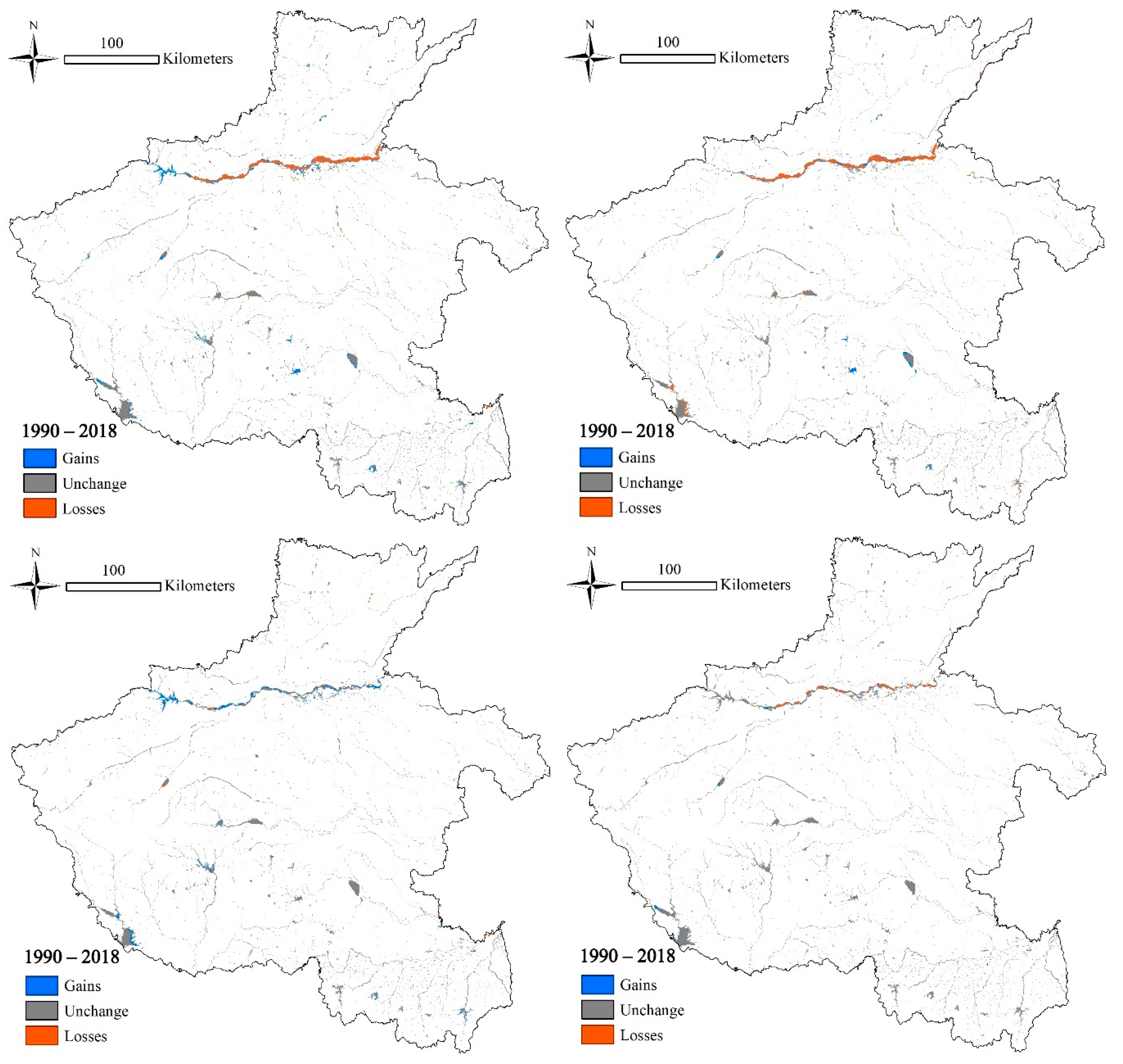
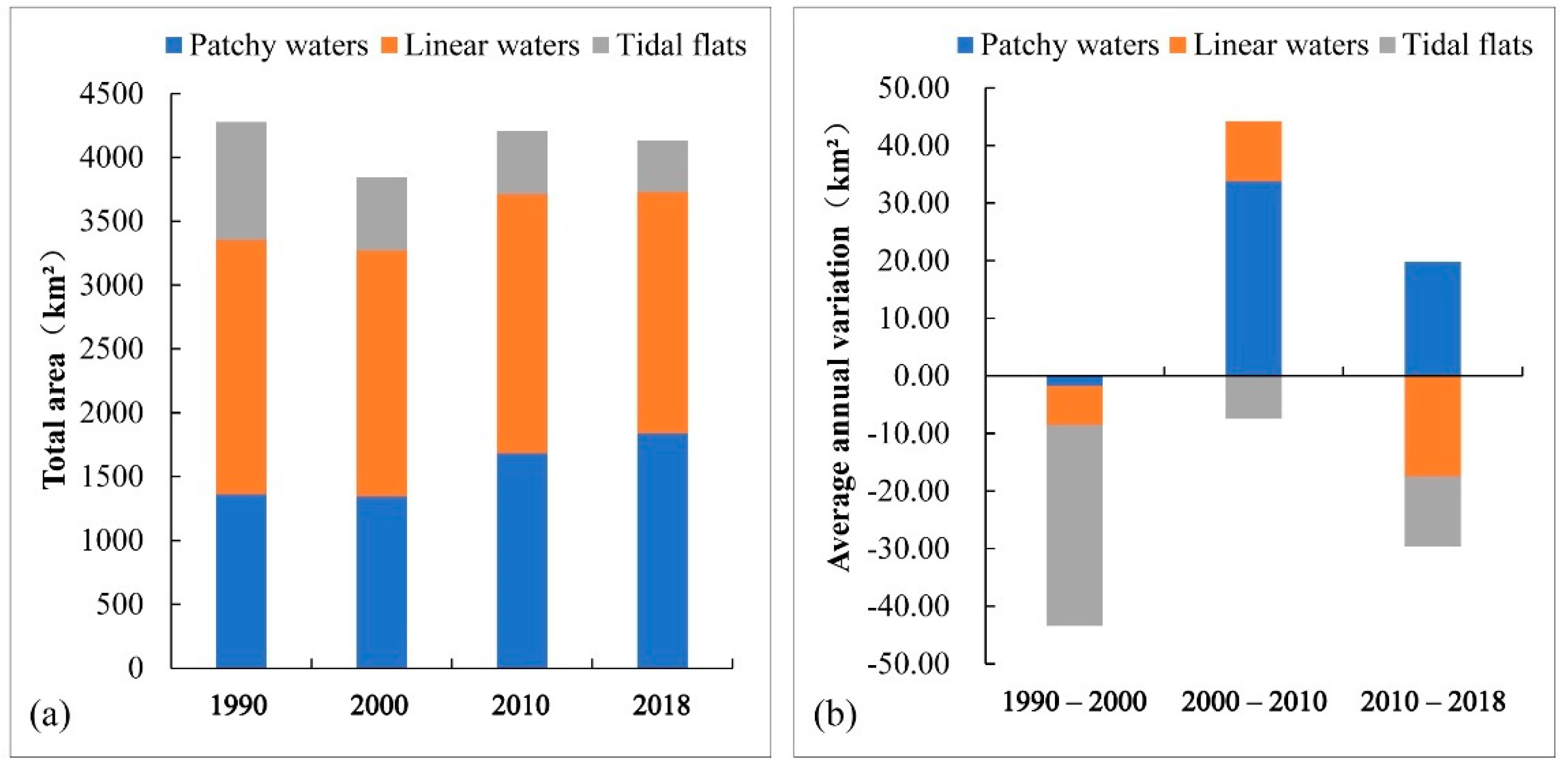
3.1. Dynamic Changes of Surface Waters

The surface waters of Henan Province are more prevalent in the south than in the north (Supplementary Materials Figure S1). Among these waters, patchy waters (lakes, reservoirs, and ponds) are distributed mainly in the low mountainous area in the southwest, linear waters (rivers and canals) are distributed mainly in the eastern plains, and tidal flats are distributed mainly along the Yellow River and around large lakes. From 1990 to 2018, surface waters in this region changed dramatically (Figure 2). In particular, there was a significant loss in tidal flats with an increase in developed land and crop land, and a gain in patchy water spaces (lakes, reservoirs and ponds) at the expense of crop land (Figure 3a). The total area of surface waters in the region was reduced by 145.30 km2. The average annual variations of three-time sub-intervals (1990–2000, 2000–2010, and 2010–2018) were −43.39, 36.74 and −9.85 km2, respectively. In terms of surface waters in the region, there was an initial decrease in river water area and tidal flats in 1990–2000, an increase in primarily patchy waters (by 337.74 km2, accounting for 70.59% of the total increase) in 2000–2010, and a decrease in linear waters and tidal flats accompanied by an increase in patchy waters in 2010–2018 (Figure 3b).
Among the average annual variations of each water type in different cities (Figure S2), the losses of linear waters occurred mainly in Nanyang, Sanmenxia, Zhengzhou, Xinxiang, Zhumadian, Jiaozuo and Luoyang during the 2010–2018 period, considerable decreases in tidal flats occurred mainly in Zhengzhou, Xinxiang, Kaifeng and Jiaozuo during the 1990–2000 and 2010–2018 periods, and increases in patchy waters occurred mainly in Luoyang, Zhumadian, Nanyang, Jiyuan and Zhengzhou during the 2000–2018 period.

3.2. Landscape Transition of Surface Waters

The landscape conversion matrix is shown in Table 5 and Table S1. Considering the result of the patch change analysis performed in ArcGIS 10.2, from 1990 to 2018, the total conversion water area was 1865.12 km2, 44.59% of the total surface water area in 1990. The loss in water area was 778.49 km2, with large conversion from tidal flats (320.43 km2) and linear waters (241.26 km2) to crop land. The increase in new waters was 668.01 km2, with large conversion from crop land to patchy waters (353.32 km2) and linear waters (115.50 km2). It is also noteworthy that 21.47% of the loss of patchy waters was attributable to conversion to developed land. The area associated with this conversion was largest during the 2000–2010 period. The conversion area among the different types of surface waters was 418.62 km2, with conversion occurring mainly from tidal flats to linear waters (161.67 km2) and patchy waters (112.23 km2). Among the different time periods (Table S1), the total water-to-land conversion area was largest in 1990–2000 (1272.49 km2). The area of water loss was also highest during the 1990–2000 period, with substantial conversion of tidal flats (−270.76 km2) and linear waters (−191.36 km2) to crop land. Water-area increases occurred mainly during the 2000–2010 period (+507.02 km2), with substantial crop land conversion to patchy waters (+213.75 km2). The areas of land converted to the different water types in the three periods were 397.48, 227.07 and 205.57 km2, respectively, showing a trend of progressive decrease. Water self-conversion occurred mainly from tidal flats to linear waters (162.94 km2) and from patchy waters to tidal flats (104.00 km2) during the 1990–2000 period, and then from tidal flats to patchy waters (108.58 km2) during the 2000–2010 period.

3.3. Landscape Pattern Changes in Surface Waters

Dynamic changes in the surface water pattern in terms of landscape dominance, fragmentation and connectivity were evident in the province, as demonstrated by the six landscape- and class-level metrics (Figure 4). There was no difference in the change trend of landscape pattern by using the 8 cell or 4 cell neighborhood rule to compute these metrics. However, values of PD, MESH and ENN_MN exhibited a larger landscape fragmentation and a shorter neighbor distance between different patches by using the 4 cell neighbor rule. Trends in PD (Figure 4a) and MESH (Figure 4e) reflected a decrease in landscape fragmentation through the conversion of large patches of crop land and tidal flats to patchy waters. The MESH values also showed that the effective mesh size of patchy waters exceeded the size of linear waters after 2010. Additionally, the LPI of patchy waters increased rapidly after 2000 (Figure 4b). The trend in IJI at landscape level reflected an increase from 1990 to 2010 dominated by linear waters, whereas a decrease trend from 2010 to 2018 was influenced by the decline of patch adjacency of all water cover types (Figure 4c). The IJI of tidal flats was the largest among all water cover types, and had a decreasing trend after 2000. The trends in ENN_MN reflected a rapid increase in patch neighbor distance between 2000 and 2010 (Figure 4d). Linear waters had the lowest value of IJI and ENN_MN, the largest value of COHESION, and dominated the trends in surface water connectivity at the landscape level during the 1990–2010 period. Patchy waters had the largest LPI in 2010, the most rapid growth in COHESION and IJI during the 2000–2010 period, and dominated the increasing trends in surface water connectivity at the landscape level after 2000, counteracting the negative effects of the significant reduction in tidal flat area.

3.4. Changes in Surface Water Spatial Connectivity

Dynamic changes in surface water spatial connectivity in Henan Province over the past three decades were assessed using four global-level (Table 6), two component-level (Figure 5 and Figure 6), and three local-level graph metrics (Figure 7, Figure 8, Figure 9, Figure 10 and Figure 11).

3.4.1. Global-Level Analysis

From 1990 to 2018, the graph connectivity of surface waters exhibited a decreasing trend, with negative growth in EC, SLC, and IIC at the global level (Table 6). Their variation trends indicated the largest reduction in surface water connectivity from 1990 to 2000 and a large increase from 2000 to 2010. From the combination of the four graph metrics and the areal change trends of the various surface waters (Figure 3), during the 1990–2000 and 2010–2018 periods, the number of components increased significantly, probably due to the disappearance of large areas of tidal flats along the Yellow River and linear waters in western mountainous area. The decline in NC from 2000 to 2010 was possibly due to the increase in patchy water areas and connected water patches.

3.4.2. Component-Level Analysis

The distributions of IIC (Figure 5) and EC (Figure 6) at component level indicated that the Yellow River had the highest integral index of connectivity and equivalent connectivity during the entire time, followed by the catchments of the Danjiang, Huai, Shaying, Tangbai, and Ru Rivers, respectively. The largest values of IIC and EC at the component level exhibited a gradual decreasing trend, with the first decline between 1990 and 2000 and the second between 2010 and 2018. The lowest values of IIC and EC were observed in 2000, probably because of construction related to the Xiaolangdi Water Conservancy Project along the Yellow River during the 1997–2001 period.

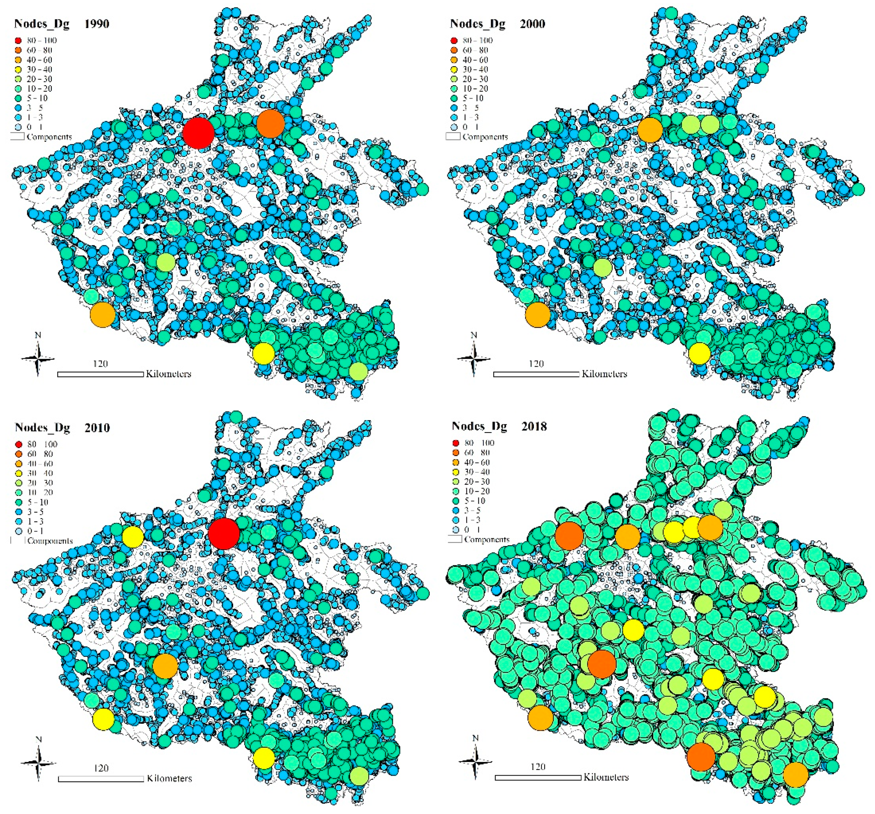
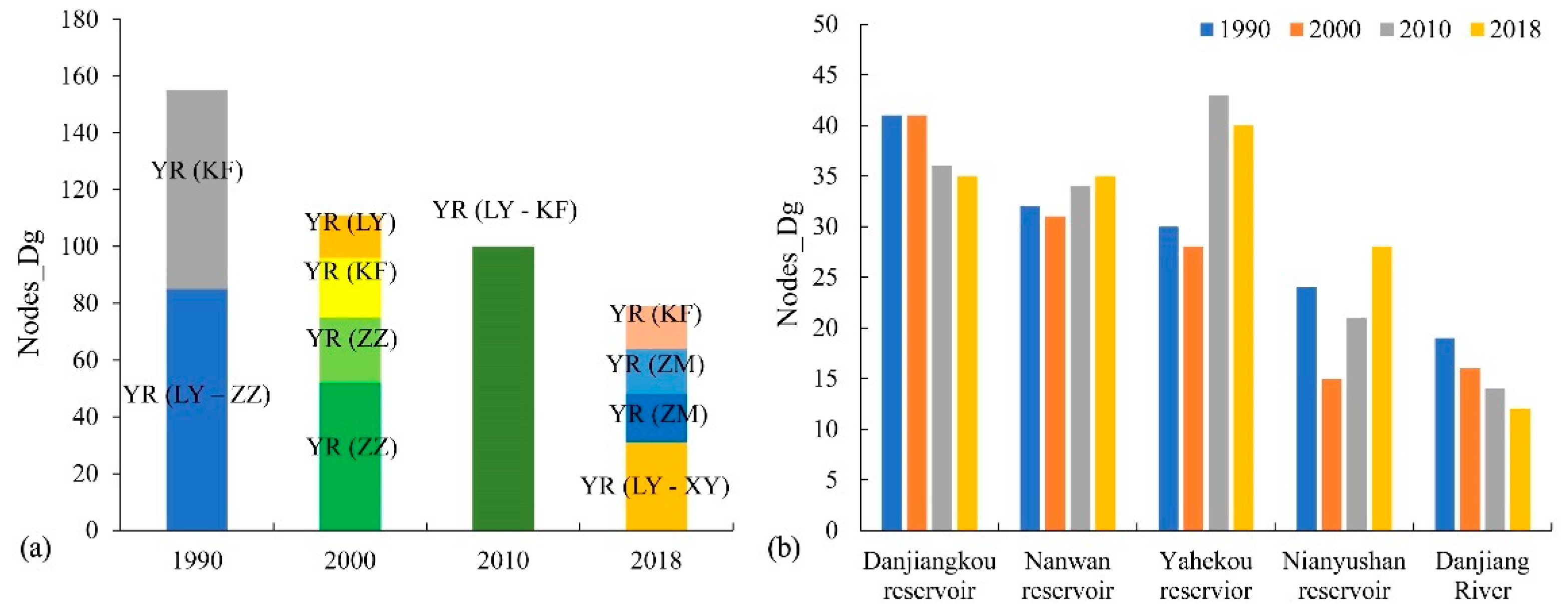
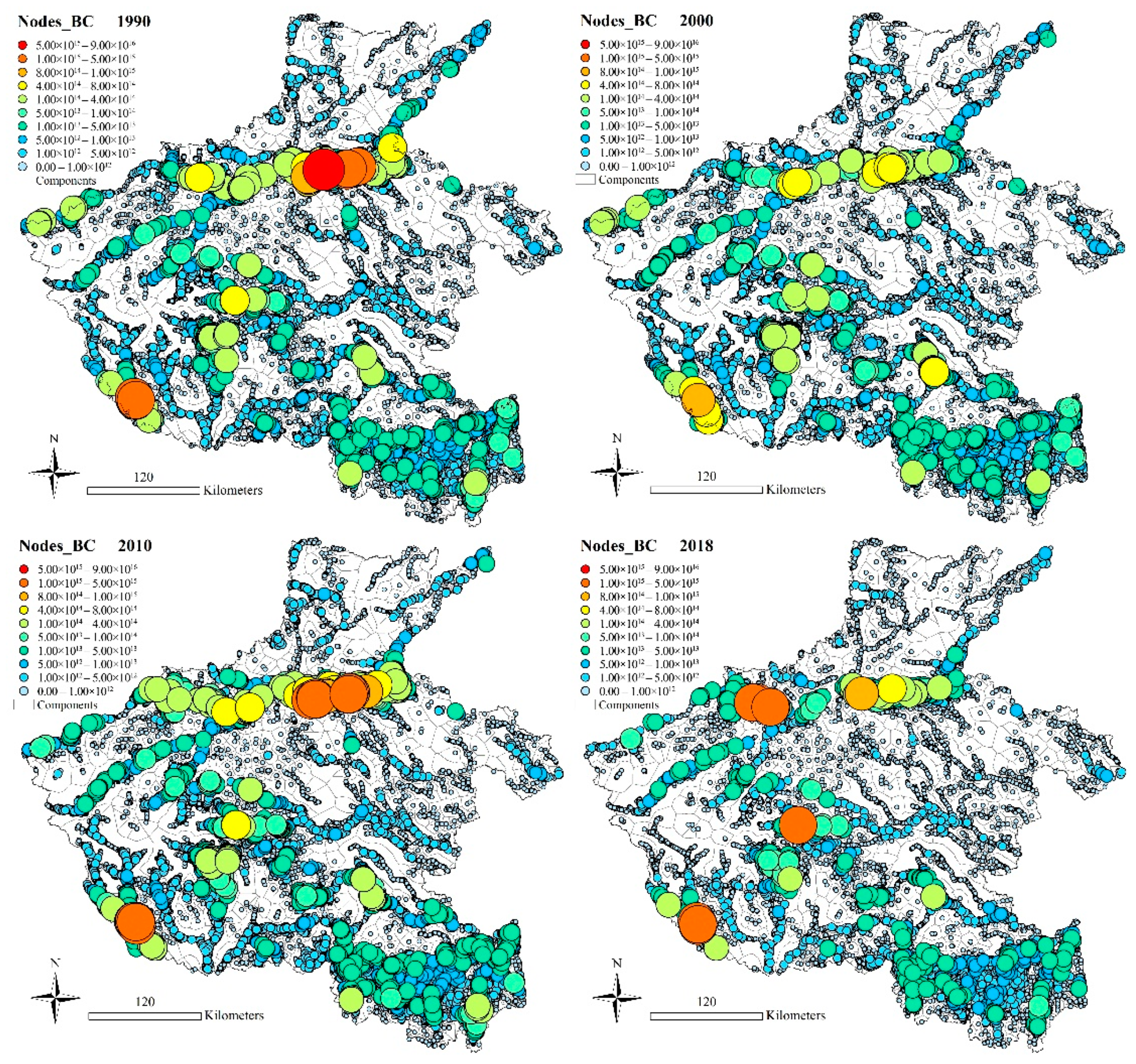
3.4.3. Local-Level Analysis

The contribution of each water patch to overall water spatial connectivity was measured using three local- and delta-level graph metrics (Figure 7, Figure 8, Figure 9 and Figure 10). The Yellow River had the largest node degree index values throughout the study period of 1990–2010 (Figure 7), while Xiaolangdi Reservoir had the largest Dg value in 2018. Patchy waters had higher node degree values, and they play the hub role in the overall connectivity of surface water bodies. The other top five patches with higher Dg values in 1990 were the Danjiangkou Reservoir in Nanyang, Yahekou Reservoir in Nanyang, Nianyushan Reservoir in Xinyang, and Danjiang River in Nanyang. Among these nodes, from 1990 to 2018, the node degree of the Xiaolangdi Reservoir increased from zero to the most, whereas that of the Yellow River decreased and changed the most (Figure 7). Furthermore, the Yellow River was seriously fragmented into several sections in 2000 and 2018 (Figure 8a). The Dg of the Danjiangkou Reservoir and Danjiang River also exhibited some reduction, while Nanwan, Yahekou, and Nianyushan Reservoirs exhibited some increase (Figure 8b). The water body with a higher betweenness centrality index of stepping stone patches was mainly concentrated between the reservoirs and the rivers (Figure 9). The size of these patches was relatively small. The position of these patches also changed frequently. The largest value of BC decreased firstly (1990–2000) and then increased from 1990 to 2018, and finally decreased by 35.78% compared with 1990.
In an analysis wherein one node was removed at a time, the relative importance of each water patch was assessed based on the dPC metric at the delta level (Figure 10). The Yellow River was the most important water patch for overall water spatial connectivity. Other patches including Danjiangkou Reservoir (second in 1990, 2000, and 2018, third in 2010), Xiaolangdi Reservoir (second in 2010 and third in 2018), and Suyahu Reservoir (third in 1990 and 2000) were the top three most important graph nodes for the total water spatial connectivity in Henan Province (Figure 11). The change trend of dPC showed that the relative importance of the Yellow River decreased dramatically in 1990–2000 and 2010–2018, probably due to the construction of the Xiaolangdi Reservoir and its regulation of the water quantity in the Yellow River. The relative importance of the Danjiang increased during 1990–2000 and 2010–2018. The relative importance of the Xiaolangdi Reservoir increased from none to the second level in 2010 and the third level in 2018.

4. Discussion

The results from this study reflected the dynamic changes and evolution processes of the surface waters and their structural connectivity in Henan Province from 1990 to 2018 and helped with identifying the hubs, stepping stones and relatively important water patches that need to be protected and developed in future spatial pattern optimization and high-quality development of the water environment in Henan Province. The use of a combination of approaches (GIS spatial analysis, landscape pattern analysis, graph connectivity analysis) constitutes a reference model for other similar studies.

4.1. Surface Water Pattern Dynamics and Relevant Influencing Factors

Surface waters in Henan Province exhibited fluctuating decrease trends, attributable mainly to a loss in linear waters during the 2010–2018 period, a gain in patchy waters during the 2000–2010 period, and a considerable decrease in tidal flats (patches along the Yellow River) (Figure 2 and Figure 3), which were converted to crop land during 1990–2000 (Table 5 and Table S1). This is mainly because the water-sediment regulation of the Xiaolangdi Reservoir in the Yellow River stabilized the water level, and a large number of flood lands were reclaimed for farming [47]. The results of landscape metrics reflected a decrease in landscape fragmentation (Figure 4a,e) due to the disappearance of a large number of isolated and broken tidal flat patches and the growth of large patchy water patches. The landscape dominance of patchy waters was dramatically increased after 2000 (Figure 4b), and they dominate the growth of landscape connectivity (Figure 4c,f) and offset the impact of the steep decline in the patch cohesion index of the tidal flats on the overall landscape connectivity (Figure 4f). However, the distance between patches was increased as well due to the loss of rivers. Trends of ENN_MN at landscape and class level (Figure 4d) indicated that the nearest neighbor distance and shortest paths between water patches were increasing from 1990 to 2018. This indirectly reflected the decrease in the structural connectivity of surface water bodies. Graph metrics at global level (Table 6) also confirmed these change trends in surface water graph connectivity.
The conversion matrix (Table 5 and Table S1) presented two situations. One was the conversion between water bodies and other land, mainly from tidal flats and linear waters to crop land as a compensation for the encroachment of urban land onto crop land and from crop land to patchy waters to meet the needs of economic and population growth. There was also some conversion from patchy water patches to construction land. This may have been caused by the activity of “lake filling for urban construction” during the rapid urbanization process [9]. New urban water bodies were also excavated during the construction of new towns, such as the North Long lake (6.08 km2) in Zhengdong New District, and Feng lake (0.77 km2) in Xinxiang Plain New Area. The other was conversion between different water types, mainly from tidal flats to linear waters or patchy waters, that was probably caused by changes in timings of precipitation, and the expansion of aquaculture farming [48].
Correlation analysis (Table S2) revealed that the patchy water area was positively correlated with economic level (per-capita GDP) and urbanization rate, whereas tidal flat area and pattern (LPI, COHESION, and MESH) was negatively correlated with population size. There was also a positive correlation between the urbanization rate and surface water pattern (ENN_MN of linear and patchy waters, COHESION and MESH at landscape level). Population growth, rapid economic development and urbanization have increased the wasteland cultivation, aquaculture farming pond excavation and reservoir construction for water resource collection and management. The increase in patchy water area and decrease in tidal flat area had a strong influence on landscape fragmentation and connectivity. This indicated that surface water area was more influenced by human construction activities. For example, the rapid expansion of urban construction land consumed water patches in the suburbs of cities, increased the impervious surface area [49], and increased the neighbor distance between water patches. The construction related to the Xiaolangdi Water Conservancy Project [50] and the middle route of the South–North Water Diversion Project [51] had a great influence on the spatial pattern of water bodies in Henan Province, especially the Yellow River and Danjiangkou Reservoir. In addition, the IJI of patchy waters was negatively correlated with the rainfall. This is probably due to the decrease in rainfall which has resulted in the disappearance of some seasonal rivers and the fall of the patchy water level, which increased the isolation of patchy water patches.
The topography also influenced the spatial distribution and connectivity of surface waters. For example, shallow hilly areas have more patchy waters and higher water spatial connectivity, whereas plain areas have more linear waters and tidal flats, and lower water spatial connectivity due to the influence of urban construction and agricultural development. Previous studies also revealed that urban expansion had a significant impact on surface water bodies [52].

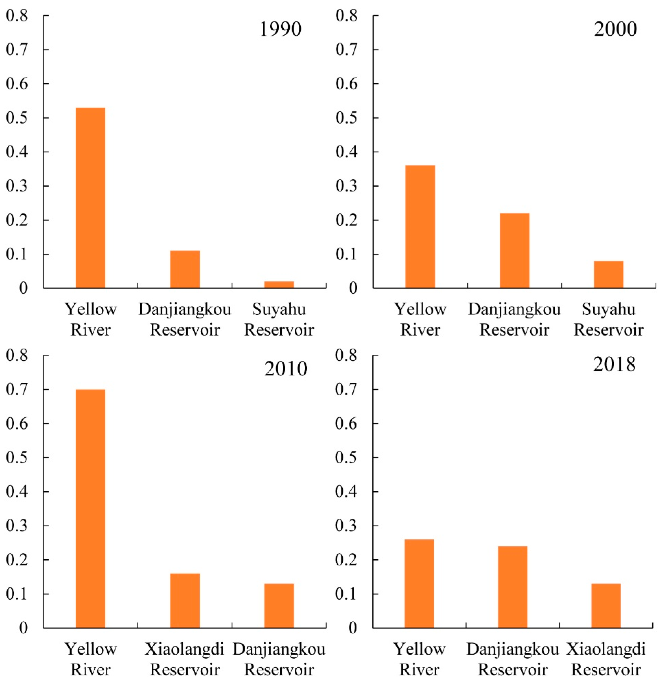
4.2. Surface Water Graph Connectivity Dynamics and Identification of Key Patches

Graph metrics are commonly used to measure and monitor changes in landscape structure connectivity, and can also provide valuable data for evaluating human construction activities and optimizing the landscape pattern [30,36,53]. In our study, graph metrics helped to illustrate the dynamic changes in surface water structure connectivity in Henan Province over the past three decades, identify hubs and stepping stones, and indicate the relative importance of water patches and key catchments for overall connectivity, making up for the deficiencies of landscape metrics at the local and component levels. The graphs at the component and local levels can provide accurate locations of key areas and important patches for future water-pattern optimization. Our results showed that patchy waters in the catchments of the Yellow, Danjiang, Huai, Shaying, Tangbai, and Ru Rivers play very important roles in the water pattern and spatial connectivity of the whole province, especially the Yellow River and Danjiangkou Reservoir. The importance of each water patch to the overall water-space connectivity changed considerably under the impacts of human construction activities and socioeconomic development. The Yellow River had the largest node degree index throughout the study period (Figure 7) and acts as a hub in terms of overall water connectivity in Henan Province. The water patches with the highest betweenness centrality index (Figure 9), mainly concentrated between the reservoir and the river, changed over time and act as the foremost stepping stone in terms of integral water connectivity in Henan Province. According to the removal analysis, from 1990 to 2018, the relative importance of the Danjiangkou Reservoir increased significantly, whereas that of the Yellow River declined (Figure 11). This may be related to the construction of the middle route of the South–North Water Diversion Project. Danjiangkou Reservoir, as the source of the middle route of the South–North Water Transfer Project, has received more attention and protection in recent years [27]. The Yellow River was fragmented into serval sections in 2000 and 2018 due to the construction of Xiaolangdi Reservoir and its regulation of water quantity. These results provide reference and point out the important objects for future optimization and development of the water spatial pattern in Henan Province.

4.3. Method Applicability and Future Work

In this study, land-cover change detection based on GIS spatial analysis combined with the application of landscape metrics and graph metrics was used to analyze the dynamic changes of surface water bodies in spatial pattern and structural connectivity during the past decades. Those theories and methods have been widely used in many previous studies. For instance, LULC combined with landscape metrics is often used to analysis the spatial-temporal dynamics of landscape pattern [22,24]. Any change could be perceived by examining variations in the metrics over time [26]. Graph metrics are often calculated based on a land-cover dataset to analyze the landscape connectivity and identify key habitats for a certain purpose [44,54]. Previous studies have used the migration distance of a species to determine the connection threshold in the parameter settings [33,55]. However, the migration distance and ability of different species in the same landscape type is not the same. It is difficult to determine a general distance for creating graphs. Some scholars have combined the morphological analysis of forest spatial patterns with graph metrics for analyzing forest structural connectivity [31]. Considering that both landscape metrics and graph metrics are quantified and calculated based on topological and morphological relations between patches and classes, there are few studies on surface water structure connectivity by combining landscape metrics with graph metrics. Here, we connected landscape metrics and graph metrics to analyze the surface water patterns and changes in structural connectivity in a significant and innovative manner. We used the mean Euclidean nearest-neighbor distance (ENN_MN) landscape metrics to determine the maximum distance and connection threshold from edge to edge between water patches in the graph creation process, which provides a simple method for the determination of distance threshold. It is also applicable to other landscape types. The integrated application of multiple methods is the development trend in the future. We will explore the relevance between landscape metrics and graph metrics through various landscape types and spatial scales over a longer time period.

5. Conclusions

This study characterized the spatiotemporal changes in surface water pattern and connectivity in Henan Province using multiple methodologies (GIS spatial analysis, landscape pattern and graph connectivity) and highlighted the relationships between landscape metrics, graph metrics, socioeconomic development level, and water conservancy construction during the rapid urbanization process between 1990 and 2018. The surface water area exhibited a decreasing trend, and most of the surface water loss was due to conversion to crop land as compensation for land consumed by urban development. Most of the increase in patchy waters came at the expense of crop land as a result of the requirements of the aquaculture industry and new urban environment construction. The large change in the Yellow River water area was caused by construction related to the Xiaolangdi Water Conservancy Project, which was the main reason for the dramatic changes in water pattern and connectivity in 2000. The Danjiangkou Reservoir and Danjiang River had the greatest increases in relative importance, possibly due to the decline of the Yellow River node degree and the construction of the middle route of the South-to-North Water Diversion Project. As a water source, the Danjiangkou Reservoir has become progressively more important to the overall water spatial pattern and connectivity in Henan Province. Human construction activity was the key driving force of surface water pattern dynamic changes, especially these main rivers and reservoirs, which play the hub, stepping stone and relatively important role in overall water landscape connectivity. In future high-quality development of surface waters in Henan Province, more attention should be paid to the scientific layout of the surface waters and the quantitative analysis of their spatial pattern and connectivity. To make scientific decisions and construct a complete, connected surface water network system, graph metric analysis suggested giving priority to the protection of hubs (high Dg) and relatively important (high dPC) patches and the development of stepping stone (high BC) patches.

Supplementary Materials

The following are available online at https://0-www-mdpi-com.brum.beds.ac.uk/article/10.3390/land10050471/s1, Figure S1: Classification and distribution maps of various surface water bodies in Henan Province in 1990, 2000, 2010, and 2018. Figure S2: Average annual variations in surface waters in different cities during different periods (1990–2000, 2000–2010, 2010–2018, and 1990–2018). Table S1: Conversion matrix of land use in different time periods from 1990 to 2018. Table S2: Correlation analysis between socioeconomic factors, precipitation, water area, landscape metrics, and graph metrics in the Henan Province region.

Author Contributions

Conceptualization, B.M. and Y.Z.; methodology, B.M. and A.L.M.; software, G.X., M.H., Y.W., P.Y. and H.X.; validation, G.T. and Y.Z.; formal analysis, B.M.; investigation, G.X., M.H., Y.W., P.Y. and H.X.; resources, B.M.; data curation, B.M.; writing—original draft preparation, B.M.; writing—review and editing, Y.Z. and A.L.M.; visualization, B.M.; supervision, Y.Z. and A.L.M.; project administration, B.M.; funding acquisition, B.M. All authors have read and agreed to the published version of the manuscript.

Funding

This research was funded by the National Natural Science Foundation of China (51808198), by the Key Scientific Research Projects Foundation of Henan Educational Committee (18A220003), and by the Science and Technology Innovation Foundation of Henan Agricultural University (30500546).

Data Availability Statement

Not applicable.

Conflicts of Interest

The authors declare no conflict of interest.

References

  1. Wang, Y. Urban land and sustainable resource use: Unpacking the countervailing effects of urbanization on water use in China, 1990–2014. Land Use Policy 2020, 90, 104307. [Google Scholar] [CrossRef]
  2. Deng, X.; Huang, J.; Rozelle, S.D.; Zhang, J.; Li, Z. Impact of urbanization on cultivated land changes in China. Land Use Policy 2015, 45, 1–7. [Google Scholar] [CrossRef]
  3. Liu, J.; Kuang, W.; Zhang, Z.; Xu, X.; Qin, Y.; Ning, J.; Zhou, W.; Zhang, S.; Li, R.; Yan, C.; et al. Spatiotemporal characteristics, patterns, and causes of land-use changes in China since the late 1980s. J. Geogr. Sci. 2014, 24, 195–210. [Google Scholar] [CrossRef]
  4. Liu, Y.; Long, H.; Li, T.; Tu, S. Land use transitions and their effects on water environment in Huang-Huai-Hai Plain, China. Land Use Policy 2015, 47, 293–301. [Google Scholar] [CrossRef]
  5. Ming, D.; Meng, J.; Xiaotai, N.; Ju, R. Analysis of evolution characteristics of urban water system form based on remote sensing data. Eng. J. Wuhan Univ. 2016, 49, 16–21. [Google Scholar]
  6. Xinran, N.; Rong, L.; Aiqiu, N.; Huafeng, L.; Rongjie, T. The change map and dynamic monitoring of lake area in Nanchang city in recent 30 years. Geomat. Spat. Inf. Technol. 2018, 41, 117–122. [Google Scholar]
  7. Wen, Y.; Kai, Y.; Qi, X.X. Effect of urbanization on growth of Shanghai river function and stream structure. Rrsources Environ. Yangtze Basin 2005, 14, 133–138. [Google Scholar]
  8. Yu, H.; Song, Y.; Chang, X.; Gao, H.; Peng, J. A Scheme for a sustainable urban water environmental system during the urbanization process in China. Engineering 2018, 4, 190–193. [Google Scholar] [CrossRef]
  9. Wu, J.; Luo, J.; Tang, L. Coupling relationship between urban expansion and lake change—A case study of Wuhan. Water 2019, 11, 1215. [Google Scholar] [CrossRef] [Green Version]
  10. Wu, P.; Tan, M. Challenges for sustainable urbanization: A case study of water shortage and water environment changes in Shandong, China. Procedia Environ. Sci. 2012, 13, 919–927. [Google Scholar] [CrossRef] [Green Version]
  11. Pan, X. The theoretical innovation and practical significance of the theory about “Two Mountains” by Xi Jinping. IOP Conf. Ser.: Earth Environ. Sci. 2018, 199, 022047. [Google Scholar] [CrossRef] [Green Version]
  12. Li, F.; Li, X.; Zhang, H. Understanding and thinking of intelligent water conservancy in China under the background of informatization. IOP Conf. Ser.: Earth Environ. Sci. 2021, 643, 012102. [Google Scholar] [CrossRef]
  13. Modica, G.; Praticò, S.; Di Fazio, S. Abandonment of traditional terraced landscape: A change detection approach (a case study in Costa Viola, Calabria, Italy). Land Degrad. Dev. 2017, 28, 2608–2622. [Google Scholar] [CrossRef]
  14. Xu, X.; Liu, J.; Zhang, S.; Li, R.; Yan, C.; Wu, S. Remote sensing monitoring dataset of multi-period land use and land cover in China (CNLUCC). Data Regist. Publ. Syst. Data Cent. Resour. Environ. Sci., Chin. Acad. Sci. 2018. [Google Scholar] [CrossRef]
  15. Herold, M.; Scepan, J.; Clarke, K.C. The use of remote sensing and landscape metrics to describe structures and changes in urban land uses. Environ. Plan. 2002, 34, 1443–1458. [Google Scholar] [CrossRef] [Green Version]
  16. Fan, C.; Myint, S. A comparison of spatial autocorrelation indices and landscape metrics in measuring urban landscape fragmentation. Landsc. Urban Plan. 2014, 121, 117–128. [Google Scholar] [CrossRef]
  17. Smiraglia, D.; Ceccarelli, T.; Bajocco, S.; Perini, L.; Salvati, L. Unraveling landscape complexity: Land use/land cover changes and landscape pattern dynamics (1954–2008) in Contrasting Peri-Urban and Agro-Forest Regions of Northern Italy. Environ. Manag. 2015, 56, 916–932. [Google Scholar] [CrossRef] [PubMed]
  18. Hamad, R.; Balzter, H.; Kolo, K. Multi-Criteria assessment of land cover dynamic changes in halgurd sakran national park (hsnp), kurdistan region of iraq, using remote sensing and GIS. Land 2017, 6, 18. [Google Scholar] [CrossRef] [Green Version]
  19. Hou, L.; Wu, F.; Xie, X. The spatial characteristics and relationships between landscape pattern and ecosystem service value along an urban-rural gradient in Xi’an city, China. Ecol. Indic. 2020, 108, 105720. [Google Scholar] [CrossRef]
  20. Kevin McGarigal. FRAGSTATS Help; University of Massachusetts: Amherst, MA, USA, 2015; p. 182. [Google Scholar]
  21. Jaeger, J.A.G. Landscape division, splitting index, and effective mesh size: New measures of landscape fragmentation. Landsc. Ecol. 2000, 15, 115–130. [Google Scholar] [CrossRef]
  22. Lamine, S.; Petropoulos, G.P.; Singh, S.K.; Szabó, S.; Bachari, N.E.I.; Srivastava, P.K.; Suman, S. Quantifying land use/land cover spatio-temporal landscape pattern dynamics from Hyperion using SVMs classifier and FRAGSTATS®. Geocarto Int. 2017, 33, 862–878. [Google Scholar] [CrossRef]
  23. Liu, J.; Liu, X.; Wang, Y.; Li, Y.; Jiang, Y.; Fu, Y.; Wu, J. Landscape composition or configuration: Which contributes more to catchment hydrological flows and variations? Landsc. Ecol. 2020, 35, 1531–1551. [Google Scholar] [CrossRef]
  24. Mu, B.; Mayer, A.L.; He, R.; Tian, G. Land use dynamics and policy implications in Central China: A case study of Zhengzhou. Cities 2016, 58, 39–49. [Google Scholar] [CrossRef]
  25. Iojă, I.-C.; Osaci-Costache, G.; Breuste, J.; Hossu, C.A.; Grădinaru, S.R.; Onose, D.A.; Nită, M.R.; Skokanová, H. Integrating urban blue and green areas based on historical evidence. Urban. For. Urban Green. 2018, 34, 217–225. [Google Scholar] [CrossRef]
  26. Sun, B.; Zhou, Q. Expressing the spatio-temporal pattern of farmland change in arid lands using landscape metrics. J. Arid Environ. 2016, 124, 118–127. [Google Scholar] [CrossRef]
  27. Wang, L.; Wang, S.; Zhou, Y.; Zhu, J.; Zhang, J.; Hou, Y.; Liu, W. Landscape pattern variation, protection measures, and land use/land cover changes in drinking water source protection areas: A case study in Danjiangkou Reservoir, China. Glob. Ecol. Conserv. 2020, 21, e00827. [Google Scholar] [CrossRef]
  28. Clauzel, C.; Foltête, J.-C.; Girardet, X.; Vuidel, G. Graphab 2.4 User Manual. 2019. Available online: https://sourcesup.renater.fr/www/graphab/en/documentation.html (accessed on 1 November 2020).
  29. Foltête, J.-C.; Clauzel, C.; Vuidel, G. A software tool dedicated to the modelling of landscape networks. Environ. Model. Softw. 2012, 38, 316–327. [Google Scholar] [CrossRef]
  30. Minor, E.S.; Urban, D.L. A graph-theory framework for evaluating landscape connectivity and conservation planning. Conserv. Biol. 2008, 22, 297–307. [Google Scholar] [CrossRef]
  31. Saura, S.; Vogt, P.; Velázquez, J.; Hernando, A.; Tejera, R. Key structural forest connectors can be identified by combining landscape spatial pattern and network analyses. For. Ecol. Manag. 2011, 262, 150–160. [Google Scholar] [CrossRef]
  32. Qi, K.; Fan, Z.; Ng, C.N.; Wang, X.; Xie, Y. Functional analysis of landscape connectivity at the landscape, component, and patch levels: A case study of Minqing County, Fuzhou City, China. Appl. Geogr. 2017, 80, 64–77. [Google Scholar] [CrossRef]
  33. Liu, S.; Yin, Y.; Cheng, F.; Dong, S.; Zhang, Y. Using cross-scale landscape connectivity indices to identify key habitat resource patches for Asian elephants in Xishuangbanna, China. Landsc. Urban Plan. 2018, 171, 80–87. [Google Scholar] [CrossRef]
  34. Bishop-Taylor, R.; Tulbure, M.G.; Broich, M. Surface-water dynamics and land use influence landscape connectivity across a major dryland region. Ecol. Appl. 2017, 27, 1124–1137. [Google Scholar] [CrossRef]
  35. Saura, S.; Rubio, L. A common currency for the different ways in which patches and links can contribute to habitat availability and connectivity in the landscape. Ecography 2010. [Google Scholar] [CrossRef]
  36. Mu, B.; Li, H.; Mayer, A.L.; He, R.; Tian, G. Dynamic changes of green-space connectivity based on remote sensing and graph theory: A case study in Zhengzhou, China. Acta Ecol. Sin. 2017, 37, 4883–4895. [Google Scholar]
  37. Pascual-Hortal, L.; Saura, S. Comparison and development of new graph-based landscape connectivity indices: Towards the priorization of habitat patches and corridors for conservation. Landsc. Ecol. 2006, 21, 959–967. [Google Scholar] [CrossRef]
  38. Bodin, Ö.; Saura, S. Ranking individual habitat patches as connectivity providers: Integrating network analysis and patch removal experiments. Ecol. Model. 2010, 221, 2393–2405. [Google Scholar] [CrossRef]
  39. Saura, S.; Estreguil, C.; Mouton, C.; Rodríguez-Freire, M. Network analysis to assess landscape connectivity trends: Application to European forests (1990–2000). Ecol. Indic. 2011, 11, 407–416. [Google Scholar] [CrossRef]
  40. Minor, E.S.; Urban, D.L. Graph theory as a proxy for spatially explicit population models in conservation planning. Ecol. Appl. 2007, 17, 1771–1782. [Google Scholar] [CrossRef]
  41. Zetterberg, A.; Mörtberg, U.M.; Balfors, B. Making graph theory operational for landscape ecological assessments, planning, and design. Landsc. Urban Plan. 2010, 95, 181–191. [Google Scholar] [CrossRef]
  42. Foltête, J.-C.; Girardet, X.; Clauzel, C. A methodological framework for the use of landscape graphs in land-use planning. Landsc. Urban Plan. 2014, 124, 140–150. [Google Scholar] [CrossRef]
  43. Mu, B.; Liu, C.; Tian, G.; Xu, Y.; Zhang, Y.; Mayer, A.L.; Lv, R.; He, R.; Kim, G. Conceptual planning of urban–rural green space from a multidimensional perspective: A case study of Zhengzhou, China. Sustainability 2020, 12, 2863. [Google Scholar] [CrossRef] [Green Version]
  44. Shanthala Devi, B.S.; Murthy, M.S.R.; Debnath, B.; Jha, C.S. Forest patch connectivity diagnostics and prioritization using graph theory. Ecol. Model. 2013, 251, 279–287. [Google Scholar] [CrossRef]
  45. Liu, J.; Liu, M.; Tian, H.; Zhuang, D.; Zhang, Z.; Zhang, W.; Tang, X.; Deng, X. Spatial and temporal patterns of China’s cropland during 1990–2000: An analysis based on Landsat TM data. Remote Sens. Environ. 2005, 98, 442–456. [Google Scholar] [CrossRef]
  46. Goldberg, C.S.; Waits, L.P. Comparative landscape genetics of two pond-breeding amphibian species in a highly modified agricultural landscape. Mol. Ecol. 2010, 19, 3650–3663. [Google Scholar] [CrossRef]
  47. Xia, X.; Dong, J.; Wang, M.; Xie, H.; Xia, N.; Li, H.; Zhang, X.; Mou, X.; Wen, J.; Bao, Y. Effect of water-sediment regulation of the Xiaolangdi reservoir on the concentrations, characteristics, and fluxes of suspended sediment and organic carbon in the Yellow River. Sci. Total Environ. 2016, 571, 487–497. [Google Scholar] [CrossRef] [Green Version]
  48. Ottinger, M.; Kuenzer, C.; Liu, G.; Wang, S.; Dech, S. Monitoring land cover dynamics in the Yellow River Delta from 1995 to 2010 based on Landsat 5 TM. Appl. Geogr. 2013, 44, 53–68. [Google Scholar] [CrossRef]
  49. Gong, P.; Li, X.; Zhang, W. 40-year (1978–2017) human settlement changes in China reflected by impervious surfaces from satellite remote sensing. Sci. Bull. 2019, 64, 756–763. [Google Scholar] [CrossRef] [Green Version]
  50. Chen, J.; Zhou, W.; Chen, Q. Channel re-establishment of the Lower Yellow River in ten years operation of Xiaolangdi Reservoir. J. Hydraul. Eng. 2012, 43, 127–135. [Google Scholar]
  51. Yang, Y.; Hu, B.; Li, S. Impact from Mid-route of South-to-North Water Transfer Project on water environment along its Henan Section and study on relevant countermeasures. Water Resour. Hydropower Eng. 2012, 43, 16–18. [Google Scholar]
  52. Du, N.; Ottens, H.; Sliuzas, R. Spatial impact of urban expansion on surface water bodies—A case study of Wuhan, China. Landsc. Urban Plan. 2010, 94, 175–185. [Google Scholar] [CrossRef]
  53. Wei, Y.; Li, Y.; Weng, S.; Xu, Y.; Zhu, L. Impact of urbanization on stream structure and connectivity of plain river network in the Taihu Basin. J. Lake Sci. 2020, 32, 553–563. [Google Scholar]
  54. Girardet, X.; Foltête, J.-C.; Clauzel, C. Designing a graph-based approach to landscape ecological assessment of linear infrastructures. Environ. Impact Assess. Rev. 2013, 42, 10–17. [Google Scholar] [CrossRef]
  55. Matos, C.; Petrovan, S.O.; Wheeler, P.M.; Ward, A.I. Landscape connectivity and spatial prioritization in an urbanising world: A network analysis approach for a threatened amphibian. Biol. Conserv. 2019, 237, 238–247. [Google Scholar] [CrossRef]
Figure 1. Administrative districts and topography of Henan Province in the Central Plains Urban Agglomeration (a), and watershed map of the province (b).
Land 10 00471 g001
Figure 2. Changes and distribution of surface water bodies during the different periods from 1990–2018 in Henan Province.
Land 10 00471 g002
Figure 3. Area (a) and average annual variation (b) trends of various waters in Henan Province from 1990 to 2018.
Land 10 00471 g003
Figure 4. Analysis of surface water landscape pattern metrics at the landscape and class levels from 1990 to 2018 using 8 cell and 4 cell neighborhood rule. ((a): patch density (PD), (b): largest patch index (LPI), (c): interspersion and juxtaposition index (IJI), (d): mean Euclidean nearest neighbor distance (ENN_MN), (e): effective mesh size (MESH), (f): patch cohesion index (COHESION)).
Land 10 00471 g004
Figure 5. Integral index connectivity (IIC) of surface waters in Henan Province at the component level from 1990 to 2018.
Land 10 00471 g005
Figure 6. Equivalent connectivity (EC) of surface waters in Henan Province at the component level from 1990 to 2018.
Land 10 00471 g006
Figure 7. Node degree (Dg) of surface water patches at local level from 1990 to 2018.
Land 10 00471 g007
Figure 8. Node degree changes of the water patches with greater node degree from 1990 to 2018 ((a): Dg changes of Yellow River, YR—Yellow River, LY—Luoyang city, XY—Xingyang city, ZZ—Zhengzhou city, ZM—Zhongmou county, KF—Kaifeng city. (b): Dg changes of other top 5 patches).
Land 10 00471 g008
Figure 9. Betweenness centrality index (BC) of surface water patches at local level from 1990 to 2018.
Land 10 00471 g009
Figure 10. Integral index of connectivity (dPC) of each water patch at the delta level from 1990 to 2018.
Land 10 00471 g010
Figure 11. Change in dPC values of graph nodes that are relatively important for total water spatial connectivity.
Land 10 00471 g011
Table 1. Reclassification standard of land-use and land-cover data.
Original NodeOriginal Land UseNew Land UseNew Node
11Paddy fieldCrop land1
12Dry farm
21Forest landForest land2
22Shrub land
23Open forest land
24Other woodland
31High coverage grasslandGrass land3
32Medium coverage grassland
33Low coverage grassland
41River and canalLiner waters4
42LakePatchy waters5
43Reservoir and pond
45Intertidal zoneTidal flats6
46Bottomland
51Urban landBuilt-up land7
52Rural residential area
53Other construction land
61SandOther unused land8
63Saline and alkaline land
64Marshland
65Bare land
66Bare rock stony ground
Table 2. Landscape pattern metrics representing landscape dominance, fragmentation, and connectivity.
Landscape MetricsMeaningBrief DescriptionComputing Level
Largest patch index
(LPI)
landscape dominancePercent of total area covered by the largest patchClass
Landscape
Patch density (PD)landscape fragmentationNumber of patches per areaClass
Landscape
Effective mesh size
(MESH)
The subdivision of a landscape independent of the size, lower values indicate higher fragmentationClass
Landscape
Mean Euclidean Nearest Neighbor distance
(ENN_MN)
landscape distanceThe mean of the shortest paths between the patches of a given land-cover typeClass
Landscape
Interspersion Juxtaposition Index (IJI)landscape connectivityDistribution of patch adjacencies and isolates the interspersion or intermixing of patch typesClass
Landscape
Patch cohesion index
(COHESION)
Physical contentedness of the patches, expresses the aggregation or clumping of cover types into patchesClass
Landscape
Table 3. Graph metrics representing habitat patch importance and spatial connectivity.
Connectivity MetricsComputing LevelBrief DescriptionComputing Purpose
Size of the largest components
(SLC)
GlobalLargest capacity of components, higher values indicate larger size of component consists of connected patchesCompare the size and quantity of the connected patches at different time periods
Number of components
(NC)
GlobalNumber of components in the study area, lower values indicate higher connectivity
Integral index of connectivity
(IIC)
Global
Component
Improved connectivity for the entire graph, indicates that two points randomly placed in the study area are connectedEstimate total connectivity and determine the highly connected patch distribution at different spatial scales
Equivalent connectivity
(EC)
Global
Component
The size of a single maximally connected habitat patch
Node degree
(Dg)
LocalIndicates the ability of a patch to connect with other patchesIdentify the hub patches
Betweenness centrality index
(BC)
LocalThe potential for a patch to be crossed by a path linking other patchesIdentify the stepping stone patches
Fractions of delta probability of connectivity
(dPC)
DeltaAssess the relative importance of each graph element by computing the rate of variation in the global metric induced by each removalAssess the relative importance of each water patch to the overall connectivity
Table 4. Resistance values of different factors.
Resistance ValueLand Use/Land CoverElevation (Natural Breaks)Slope (Natural Breaks)
1Surface water20–1400–2%
20Crop land140–3162–5%
40Grass land316–5545–9%
80Forest land554–8479–14%
160Unused land847–119814–20%
320Built-up land1198–237820–50%
Weight0.40.30.3
Table 5. Land-use conversion matrix from 1990 to 2018.
Base Year
Compared Year
Land Use Area in 2018 (Compared Year) (km2)
Crop LandForest LandGrass LandLinear WatersPatchy WatersTidal FlatsBuilt-up LandOther LandTotal
Land Use Area In 1990
(Base year)
(km2)
Crop land100,823.04488.40165.30115.50353.3266.403654.002.57105,668.53
Forest land837.5525,705.03289.379.9330.714.4684.480.2326,961.76
Grass land612.34737.728324.4614.4042.726.3363.551.259802.77
Linear waters241.2638.2111.451526.9558.5048.717.535.231937.83
Patchy waters55.2215.526.1112.461223.2425.0421.100.351359.04
Tidal flats320.4310.5027.74161.67112.23235.438.459.41885.85
Built-up land585.2017.9613.855.295.870.3617,857.160.0218,485.71
Other land98.657.552.762.858.431.467.8610.86140.42
Total103,573.6927,020.888841.031849.041835.03388.1721,704.1429.92165,241.90
note:changed watersgreatly changed watersunchanged waters
Table 6. Variations in four global-level graph metrics during different periods.
Global Level
PeriodEC (km2)SLC (km2)IICNC
Variations during different periods1990–2000−391.72
(−48.08%)
−104.12
(−9.79%)
−3.79
(−64.90%)
9
(1.62%)
2000–2010324.65
(76.74%)
30.56
(3.18%)
3.20
(155.89%)
−15
(−2.66%)
2010–2018−265.90
(−35.56%)
−173.35
(−17.50%)
−2.88
(−54.90%)
38
(−6.92%)
1990–2018−332.97
(−40.87%)
−246.91
(−23.21%)
−3.47
(−59.49%)
32
(5.77%)
Publisher’s Note: MDPI stays neutral with regard to jurisdictional claims in published maps and institutional affiliations.

