Optimal Sampling Intensity in South Korea for a Land-Use Change Matrix Using Point Sampling

Abstract

To report changes in land use, the forestry sector, and land-use change matrix (LUCM), monitoring is necessary in South Korea to adequately respond to the Post-2020 climate regime. To calculate the greenhouse gas statistics observing the principle of transparency required by the Climate Change Convention, a consistent nationwide land-use classification and LUCM are required. However, in South Korea, land-use information is available from the 5th National Forest Inventory conducted in 2006 onwards; therefore, developing methods to determine historical LUCM information, including the base year required by the Intergovernmnetal Panel on Climate Change (IPCC), is essential. To determine the optimal sampling intensity for measuring systematic land-use changes and to estimate the corresponding area of land-use categories for previously unmeasured years, seven intensities—2 × 2 km to 8 × 8 km—were tested using the areas of the 3rd and 4th aerial photographs in time series for forestland, cropland, grassland, wetland, and settlements, according to their standard deviations and estimates of uncertainty. Analyses of statistical accuracy, statistical efficiency, economic efficiency, and convenience showed that a sampling intensity of 4 × 4 km was ideal. Additionally, the categorized areas of unmeasured land-use years were calculated through linear interpolation and extrapolation. Our LUCM can be utilized for developing a national greenhouse gas inventory.

1. Introduction

The increasing severity of climate change has led to a need for nations to work together to address the issue. To this end, the Paris Agreement was signed targeting Post-2020 (the new climate regime after 2020) at the 21st Conference of the Parties 21 (COP21) in December of 2015. Distinct from the Kyoto Protocol, which was adopted in 1997 and imposed regulations on developed nations to reduce greenhouse gas (GHG) emissions, the Paris Agreement expanded the obligated parties by imposing GHG reduction protocols on all participating nations [1,2]. In addition to these efforts, the Paris Agreement also strengthened the transparency of national GHG levels through the development of the GHG inventory report system, aligning with five principles—transparency, accuracy, completeness, comparability, and consistency.

Although South Korea was not required to implement GHG emission reductions and absorption under the UN Framework Convention on Climate Change (UNFCCC), it is important to establish a systematic and credible national inventory system to keep pace with the new global climate regime. Considering the worldwide effort to mitigate the repercussions of climate change, the South Korean government has pledged to reach net neutrality by 2050 [3]. For the most complete analysis of its nationally determined contributions (NDCs), the government has focused on the forestry sector. Ultimately, the developed statistical system of GHG emission and absorption data must comply with international standards to participate in the new climate regime [4], and accordingly, developing a land-use change matrix (LUCM) system for the land use, land-use change, and forestry (LULUCF) sectors will be an essential component.

The LULUCF sector calculates carbon stocks, absorption, and emissions for each category of land use (forest land, cropland, grassland, wetland, settlements, and other land types) [5]. However, in Korea, due to the lack of inventory data in the LULUCF sector and activity data on settlements and other land types, area is not calculated, and the use of converted land is not distinguished. In IPCC, three approaches are presented in a manner appropriate for land-use identification and representation, which yield the exact area in increasing order, from Approach (App.) 1 to 3. South Korea remains at the App. 1 level, an approach level that can estimate the total area of the country, while the part for land is unavailable, making it suitable for countries with limited remote sensing data.

To develop a systematic LUCM, sampling methods must be established, and the areal coverages of land-use categories for unmeasured years should be estimated [6]. Further, to develop a national GHG inventory, a policy must be adopted to maintain compatibility with global LULUCF statistics by researching diverse methods of LUCM [7].

The Intergovernmental Panel on Climate Change (IPCC) classifies GHG inventories into eight categories: energy, industrial processes, solvents, other product uses, agriculture, LULUCF, and waste [8]. Of these, the LULUCF sector requires methods for establishing systematic and credible national inventories, particularly because it has an emission offset effect by generating GHG absorption amounts. Various government agencies, however, use a six-category definition of the LULUCF—forestland, cropland, grassland, wetland, settlements, and other land types—following the IPCC policies. Accordingly, inconsistencies in the definitions of land-use categories and land-use changes have led to often incompatible and limited datasets.

Currently, carbon stocks of dead organic matter and forest soils collected in the NFI have not been evaluated as a source of carbon storage. Forest soils and litter layers require time series LUCM information containing details on whether current forests have been maintained as forests for the past 20 years, while considering the last time when carbon was constant (at least 20 years) [9]. However, South Korea lacks a unified definition of land-use classification while utilizing different area information to provide time-series LUCM information. In addition, stand biomass is calculated by including ‘forest land remaining as forest land’ without distinguishing between ‘land converted to forest land’ and ‘forest land remaining as forest land’ because of the absence of activity data for the LUCM [5]. In 2010, South Korea established the Low Carbon Green Growth Act, along with comprehensive GHG management regulations [10]. In accordance with this act, South Korea classified the national GHG stock into six categories and regulated their inventories to calculate emissions and absorption amounts. Government agencies will be tasked with calculating these national statistics of LULUCF annually; however, as designated agencies and their legal roles remain undefined, an active cooperation system between them is yet to be established.

Accordingly, the pertinent next step is to develop the legal foundation of the LULUCF GHG inventory system by defining government agencies’ roles in calculating the LUCM. To this end, the systematic sampling methods for developing the LUCM, the calculation of the areal estimates of land-use categories for unmeasured land-use years, and examinations of land-use changes during set periods are required [9,11].

In the present examination of land use, a primary research goal was to measure the land-use status changes over set periods. A secondary goal was to identify land-use types based on varying sampling intensities, as the accuracy and efficiency of any obtained LUCM product will depend heavily on the methods employed. For example, Germany has developed decadal LUCM over an 8 km unit grid [12] utilizing national forest inventory (NFI) data, as well as a land-use category decision tree based on the integration of various spatial information [13,14]. New Zealand has produced a satellite image-based land cover map and uses it to create a LUCM [15]. As such, the wall-to-wall method using satellite image data in building a national level LUCM has the advantage of representing the spatial distribution of land-use changes. On the contrary, problems such as data acquisition and preprocessing for large-capacity data processing could arise, and methods involving sampling are presented as a possible remedy to this issue. When applying the sampling method, the optimal sampling intensity for obtaining accurate and cost-effective information should be selected, while taking the population characteristics into account [16]. In particular, compared to wall-to-wall methods utilizing remote sensing data, point sampling methods for large-area investigations have been presented as cost-effective [17]. As such, the sampling intensity influences the time spent on data collection and costs associated with the number of land-use sampling points, as this value is inherently dependent upon sampling intensity.

Conversely, each nation’s National Inventory Submissions (NIR) mentions a method of calculating land-use cover during unmeasured years. According to the report, nations such as the US, Japan, Germany, Sweden, New Zealand, and Finland calculate these areas using linear interpolation and/or extrapolation statistics [15,18,19,20,21]. New Zealand, however, also incorporates surrogate data, such as the administrative data of the unmeasured mid-year, whereas Finland’s policies are unique as their final estimates are calculated by imposing yearly weighted values based on the corresponding year [22].

According to the NIR report, many nations utilize sample points of national forest resource data to develop their LUCM [20,22]. Some nations calculate the optimal sampling intensity by considering national land-use characteristics [14]. In light of the IPCC policies and other national examples, South Korea should calculate the unmeasured areal extents of each land-use category using linear interpolation and extrapolation and employ these data in creating an LUCM [5,23,24]. To establish the systematic statistics of the national GHG inventory for the LULUCF, this study analyzed the sampling intensity most adequate for LUCM development in South Korea. Based on this optimal sampling intensity obtained from the results, the current study estimated the areal extent of land-use categories for unmeasured years and attempted to develop an LUCM according to the time-series changes.

2. Materials and Methods

2.1. Data Collection

To determine the optimal sampling intensity for LUCM development, the present study employed the governing body of LUCM development, approach method, statistical method, activity material items used, and definitions of land-use categories as summarized in the 2014 NIR data of Annex I nations (US, Japan, Germany, Sweden, Finland, Australia, and New Zealand) [18,19,20,22]. Based on these summarized data, each nation’s sampling intensity methods were assessed.

In South Korea, nationwide fixed sample points were established based on a 4 × 4 km systematic sampling method from the NFI [25]. Moreover, in cases of islands and metropolitan cities with smaller areal extents, 1400 supplemental sample points were distributed every 2 km to secure sufficient data (Figure 1).

The nationwide setting of sample points means that the locations to decode the information of land use every five years of the NFI inspection cycle are determined [26]. To determine the optimal sampling intensity in the current study, the final sampling intensity was determined by considering the statistical accuracy, statistical efficiency, economic efficiency, and convenience based on various sampling intensities. Previously, the NFI applied the stratified sampling method, which involves reading aerial photography, producing forest type maps, and placing samples according to forest type. Starting with the fifth NFI, the systematic sampling method, which places samples at a 4 km unit grid from the central datum, has been conducted. The information on forest resources as well as the land-use classification of each sample point has been obtained as well. In this study, land-use classification information on 2 km grid points along with the 4 km grid natively deployed in the NFI was obtained and used as a basis for analysis of various sample intensities (seven sampling intensities: −2 × 2, 2 × 4, 4 × 6, 6 × 6, 6 × 8, 8 × 8). The national GHG inventory has to be reported from the starting year of 1990, but LUCM should be reported based on the area of the final year [9]. However, since the land area of Korea increases every year due to reclamation projects and restoration surveying, recalculation may need to be carried out every year based on the area data of the final year. Therefore, the base year for statistical composition is required. In this study, 2005 was selected as the final year considering the completion of the fourth forest aerial photography. Korea’s forest aerial photographs were taken from 1972 to 1974, from 1978 to 1980, from 1986 to 1992, and from 1996 to 2005. Land-use information between two years (1992 and 2005) can only be obtained by annual monitoring the status of land use at the same time of the year. In order to understand the nationwide land-use status for these two points of time, the degree of sampling intensity plays a significant role in obtaining reliable information on land-use changes; seven different sampling intensities were applied to create an LUCM for the two different points of time, and the appropriate sampling intensities were then selected. In other words, the information on changes in land use by category occurred in the 13 years between 1992 and 2005, and the comprehensive assessment is based on an LUCM prepared by sampling intensities.

2.2. Review of International LUCM Detection Methods

Among Annex I nations, the present study reviewed the LUCM development methods for seven countries: the US, Japan, Germany, Sweden, Finland, Australia, and New Zealand [18,19,20,22]. The results of comparisons among governing bodies, approach methods, and statistical methods of LUCM development by nation are presented in

Table 1. Comparison of government agencies responsible for overseeing land use, land-use change, and forestry (LULUCF), and methods for land-use change matrix detection by nation.

Country	Institute (LULUCF)	Method
		Approach	Statistical Method
USA	Office of Atmospheric Programs, EPA	Approach 3	Sampling
Japan	Greenhouse Gas Inventory Office of Japan	Approach 2	Administrative Statistical calibration
Germany	Bundesministerium fur Ernuhrung, Landwirtschaft (BMEL)	Approach 3	Sampling
Sweden	Swedish University of Agricultural Sciences and other six institutes	Approach 3	Sampling
Finland	Natural Resources Institute	Approach 3	Sampling
Australia	Department of the Environment and Energy	Approach 3	Wall-to-Wall
New Zealand	Ministry for the Environment	Approach 3	Wall-to-Wall
Korea	Ministry of Agriculture, Food and Rural Affairs (KFS)	Approach 3	Sampling

.

The responsible body for governing LULUCF and developing the LUCM is a government agency that deals with agriculture and the environment. According to the 2006 IPCC guidelines for establishing a national GHG inventory [9], there are three approach methods of LUCM development: classifying the total area of all land-use categories in a nation (Approach 1), monitoring land-use changes between categories (Approach 2), and appending Approach 2 with spatial information (Approach 3). The review of national methods showed that all countries used Approach 3, indicating their ability to identify and analyze land-use change spatially, except for Japan, which uses Approach 2 [27]. Japan has applied a statistical sampling approach to examine forest management areas and forest management rates using aerial imagery that determines land use and changes by allocating nationwide samples through a sample drawing method (e.g., NFI sample points). The sampling method was adopted by all nations except Australia, New Zealand, and Japan. Japan uses sample data to extract forest management rates, and the Greenhouse Gas Inventory Office of Japan detects land-use change by collecting administrative statistical data. Meanwhile, the wall-to-wall method used by Australia and New Zealand determines spatial land-use coverage based on a national-level thematic map from satellite imagery [28,29]. These two statistical methods maintain different uncertainty evaluation methods, as the methods of LUCM development differ as well.

2.3. Optimal Sampling Intensity for LUCM Detection

The current study detected LUCM for seven sampling intensities: 2 × 2 km, 2 × 4 km, 4 × 4 km, 4 × 6 km, 6 × 6 km, 6 × 8 km, and 8 × 8 km, integrated with the 3rd and 4th land-use status data collected via aerial photograph interpreting. The uncertainty of land-use categories was calculated based on the different time series of data collection. In the case of civilian control zones where access is difficult for security reasons, remote data were obtained using Landsat imagery obtained during the same year of the 3rd and 4th aerial photographs.

Expectedly, the calculations of land cover areas and uncertainty yielded different results depending on which method was used (i.e., the sample-based method or the wall-to-wall method) [17]. Following the sample-based method adopted by South Korea [26], the calculation methods for the areal extent of landcover categories were as follows:

According to the sample-based method, the area of land-use categories was estimated by Equation (1):

$$A_h=A\times P_h \left(P_h=\frac{n_h}{n}, h=1, 2, 3, 4, 5, 6\right)$$

(1)

where A is total land area, $A_h$ is the estimated area of the hth land-use category, $P_h$is the sample point ratio of the hth land-use category, n is the number of total sample points, N_h is the number of sample points of the hth land-use category, and for the h landcover types, 1 = forestland, 2 = cropland, 3 = grassland, 4 = wetland, 5 = settlements, and 6 = other.

Based on the calculation of Equation (1), the accuracy of the areal estimates of land-use categories was assessed, and the optimal sampling intensity for South Korea was determined by comprehensively evaluating statistical efficiency, economic efficiency, and the convenience of sample point selection. Equation (2) shows the formula for the standard deviation of the land-use area according to Equation (1):

$$s\left(A_h\right)=A\times \sqrt{\frac{P_h\left(1-P_h\right)}{n-1}}$$

(2)

where S(A_h) is the standard deviation of the hth category’s estimated land-use area.

According to the sample-based method, the uncertainty of land use was estimated using Equation (3):

$$U_h=\frac{s\left(A_h\right)}{A_h}\times 100$$

(3)

where U_h is the uncertainty of the hth land-use category (i.e., relative standard deviation).

To evaluate statistical efficiency for determining the optimal sampling intensity, the variance ratio in Equation (4) was used to derive the relative efficiency of land-use uncertainty estimates derived from the seven sampling intensities [30,31]:

$$RE=\frac{\left(n_1+1\right)\left(n_2+3\right)s_2^2}{\left(n_2+1\right)\left(n_1+3\right)s_1^2}$$

(4)

where $s_1^2$ and $s_2^2$ indicate the variance of uncertainty drawn from the first and the second sampling intensity, respectively; and $n_1$ and $n_2$ indicate the degrees of freedom according to the number of samples used for each sample intensity. The variance $s_1^2$ pertains to a 4 × 4 km sampling intensity since relative efficiency was compared by setting the RE of this intensity to 1. Therefore, if the calculated RE > 1, the statistical efficiency is significantly high as the variance of the first sampling intensity is lower than the second sampling intensity (i.e., 4 × 4 km) [32,33,34]. Meanwhile, if the number of sample points used for different sampling intensities was identical, the relative efficiency was obtained by calculating the variance ratio of the two sampling intensities.

2.4. Estimating Land-Use Areas in Unmeasured Years

The land-use status over a certain period must be determined for creating an LUCM. Since aerial forest photographs are not taken every year for all regions, establishing an LUCM using existing methodologies for every year is nearly impossible. Therefore, it is necessary to estimate the “middle year” when aerial forest photographs cannot be used. Until now, South Korea has taken aerial photographs on four different occasions, which constitute the only available data. Land-use changes can be obtained by combining and comparing two or more different iterations of LUCM, for example, first and second, second and third, and third and fourth. However, for the remaining “un-photographed” years, obtaining information on land-use changes as well as the land use category is not possible. Available data (including land cover maps, smart farm maps, and HYDE: History database of the Global Environment) were reviewed in relation to land-use changes, but such tasks posed difficulties in reflecting accurate figures by category for past time frames. As a result, it was reasonable to estimate the area of each category in a land-use unmeasured year by linear interpolation and extrapolation techniques, which are mathematical methods based on IPCC guidelines [9,11]. Although interpolation comprises various methods in addition to applying linear relationships, the application of linear interpolation and extrapolation was deemed reasonable since the time elapsed between the first the fourth aerial photograph was short.

In the present study, the areal extent of each land-use category was estimated by linear interpolation for 1975, 1981, 1992, and 1992–2005 when land-use information databases were established through aerial photograph interpretation. Estimates for the years 1970–1974 (before the first aerial photographs were taken), and between 2006–2010 (after the fourth aerial photographs were taken) were drawn from linear extrapolation. Between the years 1970 and 2010, land use was not measured for 37 years, and for the occasions where aerial photography readings do not exist, the total land area based on national statistics for the base year was set and adjusted by linear interpolation and extrapolation techniques. Finally, the total area of each land use category was adjusted by the area ratio for each land use category in each estimated year to match the total land-use area, thus estimating the area for each land use category for each unmeasured year.

3. Results

3.1. Detection of the Land-Use Change Matrix by Sampling Intensity

To optimally detect land-use changes, LUCMs for the seven sampling intensities analyzed were created using interpreted information from the land-use data of the 3rd and 4th time series. The land use information of the sample points was analyzed by overlapping the location information of the fixed sample points placed in the 5th NFI over the aerial photographs taken in the 3rd (1862–1992) and 4th (1996–2005) iterations.

Table 2. Land-use change matrices of optimal sample point units by sampling intensity from analyses of the 3rd (1992) and 4th (2005) aerial images.

$\mathbf{Sampling} \mathbf{Intensity}: 2 \times 2 \mathrm{km}$
Inventory Number	Third (1992)
Fourth (2005)	Land Use Category	Forestland	Cropland	Grassland	Wetland	Settlement	Total
	Forestland	14,764	283	66	28	29	15,170
	Cropland	181	5440	21	29	19	5690
	Grassland	17	26	143	9	5	200
	Wetland	30	50	5	709	6	800
	Settlement	228	431	43	34	1113	1849
	Total	15,220	6230	278	809	1172	23,709
Sampling Intensity: 4 $\times$ 4 km
Number of Inventory	Third (1992)
Fourth (2005)	Land Use Category	Forestland	Cropland	Grassland	Wetland	Settlement	Total
	Forestland	3865	44	21	3	2	3935
	Cropland	13	1494	3	2	2	1514
	Grassland	3	2	22	0	1	28
	Wetland	1	12	0	186	1	200
	Settlement	52	135	18	13	253	471
	Total	3934	1687	64	204	259	6148
Sampling intensity: 6 $\times$ 6 km
Number of Inventory	Third (1992)
Fourth (2005)	Land Use Category	Forestland	Cropland	Grassland	Wetland	Settlement	Total
	Forestland	1659	36	9	3	3	1710
	Cropland	23	609	1	2	1	636
	Grassland	1	2	21	2	0	26
	Wetland	3	6	0	72	0	81
	Settlement	21	40	6	5	118	190
	Total	1707	693	37	84	122	2643

demonstrates the results of land-use change as the number of sample points for 14 years from 1992 to 2005 across different sampling intensities.

The optimal number of sample points used at the national level was 23,709 at a sampling intensity of 2 × 2 km and showed a readability of 98.3%. At 4 × 4 km, the number of sample points was 6148, with a readability of 98.1%. When a sampling intensity of 6 × 6 km was applied, the number of national sample points was 2643, with a readability of 98.2%, notably similar to the other sampling intensities. Additionally, the land-use changes by category from 1992 (3rd) to 2004 (4th) were similar; however, the number of sample points varied across the remaining four sampling intensities.

Table 3. Land-use change matrices of area (ha) by sampling intensity, as detected by analyses of 3rd (1992) and 4th (2005) aerial images.

$\mathbf{Sampling} \mathbf{Intensity}: 2 \times 2 \mathrm{km}$
Number of Inventory	Third (1992)
Fourth (2005)	Land Use Category	Forestland	Cropland	Grassland	Wetland	Settlement	Total
	Forestland	6,239,712	103,428	420	10,931	8829	6,363,321
	Cropland	61,384	2,327,962	-	9670	6307	2,405,323
	Grassland	3363	1682	55,077	-	841	60,963
	Wetland	11,352	16,397	-	295,568	2523	325,839
	Settlement	95,860	189,617	1682	14,715	470,049	771,923
	Total	6,411,671	2,639,086	57,179	330,884	488,548	9,927,369
Sampling Intensity: 4 $\times$ 4 km
Number of Inventory	Third (1992)
Fourth (2005)	Land Use Category	Forestland	Cropland	Grassland	Wetland	Settlement	Total
	Forestland	6,261,380	53,530	-	4866	3244	6,323,020
	Cropland	12,977	2,480,220	-	1622	1622	2,496,441
	Grassland	1611	3244	35,687	-	1622	42,175
	Wetland	1622	16,221	-	300,092	1622	319,557
	Settlement	85,972	222,230	-	21,088	416,885	746,175
	Total	6,363,573	2,775,446	35,687	327,668	424,995	9,927,369
Sampling Intensity: 6 $\times$ 6 km
Number of Inventory	Third (1992)
Fourth (2005)	Land Use Category	Forestland	Cropland	Grassland	Wetland	Settlement	Total
	Forestland	6,294,760	109,507	-	7552	3776	6,415,595
	Cropland	71,746	2,352,511	-	7552	3776	2,435,585
	Grassland	3776	-	75,522	-	-	79,298
	Wetland	11,328	15,104	-	264,327	-	290,760
	Settlement	79,298	169,925	3776	22,657	430,475	706,131
	Total	6,460,908	2,647,047	79,299	302,088	438,028	9,927,369

presents the LUCMs of areal units for the 3rd (1992) and 4th (2005) images’ land-use coverages according to different sampling intensities.

In the present study, 9,927,369 ha (from the 1990 standard of LULUCF reported statistics) was set as the constant national land area. At a sampling intensity of 2 × 2 km, 48,350 ha of forests were lost between 1992 and 2005, primarily from changes to settlements and croplands, corresponding to an average annual loss of ~6027 ha·yr⁻¹. For forest land, 40,553 and 45,313 ha were reduced at sampling intensities of 4 × 4 km and 6 × 6 km, respectively. Croplands underwent a significant area reduction during the analysis period, regardless of the sampling intensity applied. Grassland areas tended to increase with increasing sampling intensity, whereas wetland areal estimates were reduced. An increase in settlement areas due to sampling intensity was also observed, and although the areas varied, all other land categories were converted to settlements.

3.2. Calculation of Uncertainty in Time Series

To select the optimal sampling intensity, the areas of the 3rd and 4th aerial images in time series, standard error, and uncertainty across the five major land-use categories were calculated (

Table 4. Comparison of categorical land-use areas, standard deviations, and uncertainty estimates by examined aerial imagery and sampling intensity.

$\mathbf{Sampling} \mathbf{Intensity}: 2 \times 2 \mathrm{km}$
Survey	Categories	Forestland	Cropland	Grassland	Wetland	Settlement
Third (1992)	Area (ha)	6,411,671	2,639,086	57,179	330,884	488,548
	Standard Error	30,910.7	28,377.6	6940.5	11,704.8	13,976.1
	Uncertainty (%)	0.49	1.09	5.96	3.46	2.85
Fourth (2005)	Area (ha)	6,363,321	2,405,323	60,963	325,839	771,923
	Standard Error	30,950.6	27,535.6	5896.7	11,641.8	17,288
	Uncertainty (%)	0.49	1.16	7.04	3.48	2.23
Sampling Intensity: 4 $\times$ 4 km
Third (1992)	Area (ha)	6,363,573	2,775,446	35,687	327,668	424,995
	Standard Error	60,782.0	56,499.2	12,851,5	22,679.0	25,435.4
	Uncertainty (%)	0.96	2.07	12.44	6.88	6.08
Fourth (2005)	Area (ha)	6,323,020	2,496,441	42,175	319,557	746,175
	Standard Error	60,776.0	54,551.9	8525.6	22,463.1	33,677.4
	Uncertainty (%)	0.96	2.23	18.86	6.96	4.43
Sampling Intensity: 6 $\times$ 6 km
Third (1992)	Area (ha)	6,460,908	2,647,047	79,298	302,088	438,028
	Standard Error	92,368.8	84,948.3	22,691.3	33,880.2	40,526.3
	Uncertainty (%)	1.44	3.26	16.33	10.74	8.84
Fourth (2005)	Area (ha)	6,415,595	2,435,585	79,298	290,760	706,131
	Standard Error	92,301.7	82,560.6	19,061.6	33,289.1	49,888.0
	Uncertainty (%)	1.44	3.46	19.52	10.94	6.99

).

The observed variation in uncertainty for the forestlands, which showed a slight change in area with time, was assessed to be minimal. Accordingly, the uncertainty of forest cover maintained a level as low as 0.49–1.44% across all sampling intensities. In contrast, the uncertainty of croplands was relatively low, with the 4^th image uncertainty greater than that of the 3rd image, as the area was originally large and significantly decreased over time. Overall, the uncertainty by land-use categories at the national level remained low, even at different sampling intensities.

3.3. Optimal Sampling Intensity for LUCM Development

3.3.1. Uncertainty by Sampling Intensity

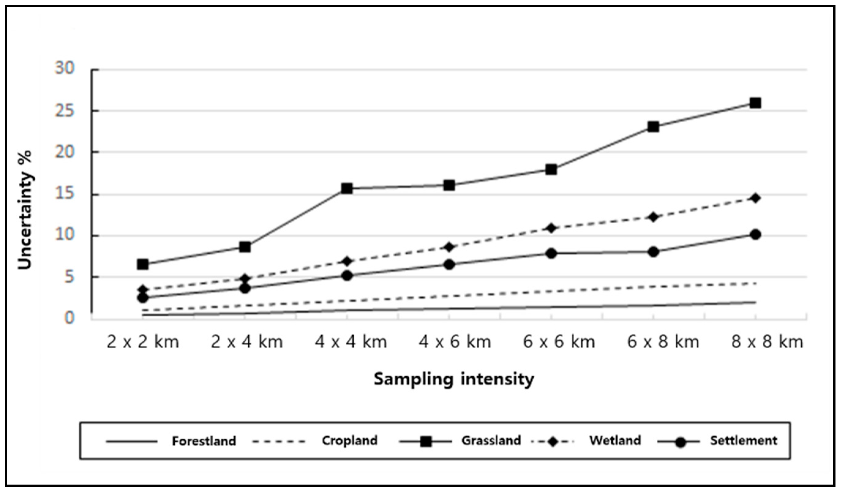
Although the uncertainty by sampling intensity according to land-use category had limited variability, differences between the 3rd (1992) and 4th (2005) time series were apparent. The comparative results by averaging the uncertainty estimates by land-use category across all sampling intensities are shown in Figure 2.

The uncertainty values for all categories at 2 × 2 km with large sampling ratios were the smallest and tended to increase as sampling intensity decreased. Forestlands maintained the highest percent coverage among all land-use categories and accordingly had the lowest uncertainty (0.49–1.94% by sampling intensity), followed by croplands (1.09–4.46% by sampling intensity). By contrast, the uncertainties of the smaller grasslands and wetlands were relatively high (3.46–19.52 by sampling intensity). Settlements demonstrated slightly higher levels of uncertainty (2.54–10.21%) than forestlands and croplands.

3.3.2. Relative Efficiency by Sampling Intensity

According to the uncertainty estimates by sampling intensity obtained above, a 2 × 2 km method maintained the lowest uncertainty; however, the optimal decision must be made in consideration of the convenience and economics of data collection, rather than accuracy alone, as the differences in uncertainty were insubstantial, even at low sampling intensities. Therefore, the present study compared estimates of the relative efficiency to determine the optimal sampling intensity after comprehensively reviewing economic efficiency and the convenience of data collection.

Table 5. Comparison of relative efficiency estimates by sampling intensity.

Sampling Intensity	$\mathit{n}$	${\mathit{s}}^2$	Relative Efficiency
2 $\times$ 2 km	10	5.05	0.31
2 $\times$ 4 km	10	8.94	0.54
4 $\times$ 4 km	10	16.46	1.00
4 $\times$ 6 km	10	30.87	1.88
6 $\times$ 6 km	10	38.69	2.35
6 $\times$ 8 km	10	66.63	4.05
8 $\times$ 8 km	10	88.09	5.37

displays the comparative results of relative efficiency by each sampling intensity’s variance ratio when relative efficiency at a standard of 4 × 4 km sampling intensity was set to 1.

The relative efficiency estimates decreased with increasing sampling intensity, showing a pattern similar to that observed for uncertainty. Consequently, although relative efficiency improved with sampling intensity, the optimal sampling level was determined by additional analyses of economic efficiency and the practicality of data collection.

3.3.3. Number of Sample Points and Convenience by Sampling Intensity

Table 6. Number of sample points per sample intensity.

Sampling Intensity	$2 \times 2 \mathbf{km}$	$2 \times 4 \mathbf{km}$	$4 \times 4 \mathbf{km}$	$4 \times 6 \mathbf{km}$	$6 \times 6 \mathbf{km}$	$6 \times 8 \mathbf{km}$	$8 \times 8 \mathbf{km}$
Sample point	24,119	12,271	6269	4121	2691	2047	1567

shows the required number of sample points to be interpreted for estimating the annual change by sampling intensity, as it is another important metric for determining the optimal sampling intensity due to the associated time and costs.

This number includes indecipherable sample points as revealed through aerial imagery analysis and tends to display an opposite pattern to that of uncertainty and relative efficiency. The analysis found that the sample points for 2 × 2 km (i.e., highest sampling intensity) were 15.39 times higher than those of 8 × 8 km (i.e., lowest sampling intensity). In South Korea, spatial land-use data have been identified every five years [26], with nationwide sample points for 4 × 4 km grids established through the NFI. The availability of NFI’s existing sample points by sampling intensity correlates with the convenience of data examination, and of the seven sampling intensities, the conveniences of 4 × 4 km and 8 × 8 km were deemed superior due to the preexistence of the NFI sample points at these levels.

3.3.4. Selection of Optimal Sampling Intensity

In the current study, four indicators—statistical accuracy, statistical efficiency, economic efficiency, and convenience—were selected and quantified through weighted values and scores of specific metrics. Following the importance of each indicator, weighted values of 40% for uncertainty (i.e., statistical accuracy), 20% for relative efficiency (i.e., statistical efficiency), 30% for sample point economic efficiency, and 10% for convenience were applied (

Table 7. Assessment indicators and quantification methods for optimal sample intensity decision.

Evaluation Index	Total Score	Point Distribution	Section
Statistical Accuracy	40	40	<3% of Mean Uncertainty of Land Use Category
		32	3–6% of Mean Uncertainty of Land Use Category
		24	6–9% of Mean Uncertainty of Land Use Category
		16	9–12% of Mean Uncertainty of Land Use Category
		8	>12% of Mean Uncertainty of Land Use Category
Statistical Efficiency	20	20	<1.0 of Relative Efficiency
		16	1.0–2.0 of Relative Efficiency
		12	2.0–3.0 of Relative Efficiency
		8	3.0–4.0 of Relative Efficiency
		4	>4.0 of Relative Efficiency
Economic Efficiency	30	30	<4000 of Sample Points
		24	4000–8000 of Sample Points
		18	8000–12,000 of Sample Points
		12	12,000–16,000 of Sample Points
		6	>16,000 of Sample Points
Convenience	10	10	Available to use NFI Sample Points
		5	Unavailable to use NFI Sample Points

). Taking the weighted values as the total scores, those for each indicator were quantified by dividing the scores into two or five stages based on estimates according to sampling intensity. Figure 3 demonstrates the results for the adequacy of each sampling intensity according to the assessment indicator scores. The sum of the sampling intensity scores of the four assessment indicators showed that a sampling intensity of 4 × 4 km (total score, 82) was optimal.

3.3.5. Estimation of Land-Use Areas for Unmeasured Years

The total land area in each time series was set at 9,927,369 ha according to the LULUCF report statistics from 1990. Based on the areal measurements of each land-use category for the four aerial images—1974, 1980, 1992, and 2005—categorical estimates of land use for the unmeasured years from 1970 to 2010 were estimated via linear interpolation and extrapolation. After applying the linear interpolation, the areal extent by land-use category for the 41 years of analysis was calculated through the adjustment of each year’s land-use category ratio, and the results are depicted in Figure 4.

The results showed that forest land areas gradually decreased between 1970 and 2010, and there were differences in the areas from the annual national statistics. Croplands increased slightly until 1980 and have decreased ever since. Conversely, grasslands constituted 0.4% of the national land area until the late 2000s but have increased since 2009. Wetland areas showed a continuous decrease of 41,324 ha over the entire analysis period, with an average annual decrease of 1008 ha, an area that is neither insignificant nor substantially large. Settlement areas substantially increased over the analysis period, growing by 711,067 ha overall, an average annual increase of ~17,343 ha, indicating the active conversion from other land types.

4. Discussion

This study reviewed sporadic land-use data of South Korea from 1970 to 2010, and used these data to determine the optimal sampling intensity and uncertainty assessment for LUCM development. The present study proposed the use of land cover data after confirming the definitions of other nation’s land-use categories and subcategories were analogous, with only slight differences according to the nation’s status.

Most nations followed the definition of “forested lands” from the UNFAO that is based on the land cover [35]. The definitions of other categories were prioritized in cases of duplicated decryptions based on land use [11], with priority given to settlements, followed by croplands, forestlands, grasslands, wetlands, and other lands. This present study gave priority to the majority land-use categories according to overlapping, spatial thematic maps. Information about LULUCF can be obtained once annual land-use data are established for any individual location over time.

The issue addressed in the present study was how to best obtain credible information on land-use change using certain sampling intensities across South Korea. Accordingly, adequate samples were selected after LUCM development by applying various sampling intensities [16]. The optimal method to detect land-use changes was selected among the seven sampling intensities analyzed—2 × 2 km, 2 × 4 km, 4 × 4 km, 4 × 6 km, 6 × 6 km, 6 × 8 km, and 8 × 8 km. Specifically, information regarding land-use change by category for the 14 years from 1992 to 2005 was derived through analyses of the seven sampling intensities and by developing LUCMs from the 3rd (1992) and 4th (2005) aerial images.

This study estimated uncertainty via statistical accuracy and relative efficiency via statistical efficiency, based on LUCM development by sampling intensity. Along with the estimation, the current study assessed the metrics of convenience according to the possible utility of South Korea’s NFI data sample points [36]. Further, the number of sample points used to decode economic efficiency by sampling intensity was comprehensively assessed.

Considering the four indicators (statistical accuracy, statistical efficiency, economic efficiency, and convenience of data collection), a sampling intensity of 4 × 4 km was shown to be the most optimal [37]. As aerial imagery was only available for four years—1974, 1980, 1992, and 2005—all other years required areal estimation by category using linear interpolation and extrapolation to obtain annual information on land-use change [8,38,39,40,41]. By doing so, a complete time series was obtained, an important prerequisite to developing the infrastructure needed to operate a systematic national GHG inventory. Although the interpolation consisted of various methods, in addition to the application of linear relationships, the joint use of both linear interpolation and extrapolation was evaluated to be adequate, as the temporal gaps in between the four aerial images were relatively small [42,43].

As the land-use change patterns between two points in time from 1970 to 2010 could now be calculated, the detection of a time series national GHG inventory, previously limited by the absence of aerial imagery for most years, was now possible. If higher resolution imagery (e.g., ultra-high-definition satellite imagers) can be obtained in the future, it is likely that the construction of more accurate interannual LUCMs will be possible.

The statistical imagery data over civilian control zones were acquired using Landsat satellite imagery, and therefore, the data can be used for the LULUCF sector activity materials in South Korea’s consistent Approach 3 level [10]. Additionally, the calculated results according to the optimal sampling intensity can help establish an LUCM with enhanced accuracy and cost-effectiveness.

To further LUCM verification methods in future research, all possible issues when implementing LULUCF development should be discovered to increase verification accuracy. Similarly, the differences between the national and estimated statistics from imagery analyses must be corrected [44]. For example, Japan and China identify areas of land-use categories using sample-based estimates to resolve this discrepancy [30], adjusting their LUCM data reported to the national values.

In this statistical correction process, the results of the final LUCM are proportionally distributed according to the national land area of the standard year selected. In the present study, the LUCM data were standardized against 1990 values and the most recent year of image analysis, 2005. The selection of a standard year must be determined by considering various policies and factors, as the LUCM results will vary accordingly.

5. Conclusions

This study was conducted to develop a method for creating a national unit LUCM using the point sampling method presented in the IPCC guidelines. To this end, various sampling intensities (seven sampling intensities: 2 × 2, 2 × 4, 4 × 6, 6 × 8, 6 × 6, 6 × 8, and 8 × 8) were established for the 3rd (1992) and 4th (2005) aerial photographs, and LUCM for the two disparate chosen years (1992 and 2005) was created to determine which sampling intensities fit best. A quantitative evaluation considering the four evaluation indicators, namely, statistical accuracy, efficiency, economic efficiency, and convenience of data collection, found that the sampling intensity of 4 km × 4 km was the best fit. The indicators used to determine the optimal sampling intensity in this work are meaningful in that they are evaluated not only by consideration of statistical accuracy and efficiency, but also by cost-effective aspects that depend on sampling intensity. It is also meaningful in that we reviewed what is the appropriate, cost-effective method for building a future LULUCF sector matrix at the App. 3 level.

The NFI’s permanent sample points for national-level LUCM data should be actively utilized for establishing national GHG inventory statistics and international reports. The areal statistics of national land-use categories derived in the present study support the acquisition of efficient data according to aerial forest and satellite imagery, as well as NFI data. The statistical results can also be utilized for NFI data when amassed every five years.

Moreover, the constructed LUCM data can address the currently problematic issue of spatial information for national government agencies’ comparison of compatibility between national spatial data materials. The LUCM can also help avoid additional land-use examinations and reduce LULUCF inventory costs; however, to adequately construct these data for South Korea, statistical compatibility through intergovernmental cooperation should be improved when developing the national GHG inventory.

The results of the pre-built spatial and statistical information of the present study can be useful for determining forest-related policies and assessing the effects of GHG emissions and reductions. If more precise LUCMs are constructed in subsequent research, South Korea’s position in all future carbon mitigation strategies can be strengthened through the improvement of national statistics credibility, as well as the construction of accurate GHG monitoring infrastructure.

References

- Dedinec, A.; Taseska-Gjorgievska, V.; Markovska, N.; Obradovic Grncarovska, T.; Duic, N.; Pop-Jordanov, J.; Taleski, R. Towards Post-2020 Climate Change Regime: Analyses of Various Mitigation Scenarios and Contributions for Macedonia. Energy 2016, 94, 124–137. [Google Scholar] [CrossRef]
- Pistorius, T.; Reinecke, S.; Carrapatoso, A. A Historical Institutionalist View on Merging LULUCF and REDD+ in a Post-2020 Climate Agreement. Int. Environ. Agreem. 2017, 17, 623–638. [Google Scholar] [CrossRef]
- Korea Forest Servic Countermeasure to Climate Change, South Korea. That Takes the Lead in the Forestry Sector Among Asian Countrie. Available online: https://www.forest.gkr (accessed on 10 March 2021).
- Brack, C.; Richards, G.; Waterworth, R. Integrated and Comprehensive Estimation of Greenhouse Gas Emissions from Land System. Sustain. Sci. 2006, 1, 91–106. [Google Scholar] [CrossRef]
- Greenhouse Gas Inventory and Researches Center (GIR). National Greenhouse Gas Inventory—Guideline for Measurement, Reporting, Verification; GIR: Seoul, Korea, 2020; p. 442. Available online: https://www.gigkr (accessed on 21 April 2021).
- McRoberts, E.; Tomppo, E.O.; Næsset, E. Advances and Emerging Issues in National Forest Inventorie. Scand. J. For. Res. 2010, 25, 368–381. [Google Scholar] [CrossRef]
- Fuchs, H.; Magdon, P.; Kleinn, C.; Flessa, H. Estimating Aboveground Carbon in a Catchment of the Siberian Forest Tundra: Combining Satellite Imagery and Field Inventory. Remote Sens. Environ. 2009, 113, 518–531. [Google Scholar] [CrossRef]
- Intergovernmental Panel on Climate Chang Good Practice Guidance for Land Use, Land-Use Change and Forestry; Institute for Global Environmental Strategies: Hayama, Japan, 2003; p. 590. Available online: https://www.ipcc-nggip.igeojp/public/gpglulucf/gpglulucf_files/GPG_LULUCF_FULL.pdf (accessed on 21 April 2021).
- Intergovernmental Panel on Climate Change (IPCC). Chapter 3. Consistent Representation of Land. In IPCC Guidelines for National Greenhouse Gas Inventorie; Institute for Global Environmental Strategies: Hayama, Japan, 2006; pp. 3.1–3.42. Available online: https://www.ipcc-nggip.igeojp/public/2006gl/pdf/4_Volume4/V4_03_Ch3_Representation.pdf (accessed on 21 April 2021).
- Korea Legislation Research Institute Enforcement Decree of the Framework Act on Low Carbon, Green Growth. 2020. Available online: https://elaw.klri.rkr (accessed on 29 July 2020).
- Intergovernmental Panel on Climate Change (IPCC). Chapter 3. Consistent Representation of Land. In Refinement to the 2006 IPCC Guidelines for National Greenhouse Gas Inventorie; Institute for Global Environmental Strategies: Hayama, Japan, 2019; Volume 2019, pp. 3.1–3.68. Available online: https://www.ipcc-nggip.igeojp/public/2019rf/pdf/4_Volume4/19R_V4_Ch03_Land%20Representation.pdf (accessed on 21 April 2021).
- German Environment Agency (Umweltbundesamt-UBA). Land-Use, Land-Use Change and Forestry. In National Inventory Report; Umweltbundesamt: Dessau-Roßlau, Germany, 2018; pp. 514–664. Available online: https://unfccc.int/documents/65712 (accessed on 21 April 2021).
- German Environment Agency (Umweltbundesamt-UBA). National Inventory Report for the German Greenhouse Gas Inventory. In CLIMATE CHANGE National Inventory Report; Umweltbundesamt: Dessau-Roßlau, Germany, 2009; p. 565. Available online: https://www.umweltbundesamt.de/sites/defalut/files/medien/publikation/long/3755.pdf (accessed on 21 April 2021).
- Und Treibhausgasinventar, W. Johann Heinrich Von Thünen-Institute (VTI). Sonderheft Inventurstudie 2008; VTI: Braunschweig, Germany, 2011; Volume 343, p. 164. Available online: https://www.thuenen.de/media/publikationen/landbauforschung-sonderhefte/lbf_sh343.pdf (accessed on 21 April 2021).
- Ministry of the Environment (ME). New Zealand’s Greenhouse Gas Inventory 1990–2019; ME: Wellington, New Zealand, 2019; p. 531. Available online: https://environment.govt.nz/assets/Publications/New-Zealands-Greenhouse-Gas-Inventory-1990-2019-Volume-1-Chapters-1-15.pdf (accessed on 21 April 2021).
- Cochran, W.G. Sampling Techniques, 3rd ed.; John Wiley & Sons: Hoboken, NJ, USA, 1977; p. 428. ISBN 978-0-471-16240-7. [Google Scholar]
- Hwang, J.H.; Jang, I.; Jeon, S.W. Analysis of Spatial Information Characteristics for Establishing Land Use, Land-Use Change and Forestry Matrix. J. Korean Assoc. Geogr. Inf. Stud. 2018, 21, 44–55. [Google Scholar]
- United States Environmental Protection Agency (US EPA). Inventory of U.S. Greenhouse Gas Emissions and Sinks: 1990–2014; US EPA: Washington, DC, USA, 2016; p. 558. Available online: https://www.epa.gov/sites/production/files/2017-04/documents/us-ghg-inventory-2016-main-text.pdf (accessed on 21 April 2021).
- Heinrich, J.; Von Thünen-Institute (VTI). Germany’s LULUCF Inventory 2017; Thünen Institute: Braunschweig, Germany, 2017; p. 6. Available online: https://literatuthuenen.de/digbib_extern/dn059229.pdf (accessed on 21 April 2021).
- Swedish Environmental Protection Agency (SEPA). National Inventory Report Sweden 2016; SEPA: Stockholm, Sweden, 2016; p. 543. Available online: https://unfccc.int (accessed on 21 April 2021).
- Official Statistics Finland (OSF). Greenhouse Gas Emissions in Finland 1990 to 2015; Ÿ OSF: Helsinki, Finland, 2016; p. 530. Available online: https://www.stat.fi/static/media/uploads/tup/khkinv/fin_un_nir_2015_2017-04-15.pdf (accessed on 21 April 2021).
- Official Statistics Finland (OSF). Greenhouse Gas Emissions Finland 1990 to 2016; Ÿ OSF: Helsinki, Finland, 2017; p. 538. Available online: https://www.stat.fi/static/media/uploads/tup/khkinv/fi_nir_un_2016_20180415.pdf (accessed on 21 April 2021).
- Yim, J.S.; Moon, G.H.; Shin, M.Y. Development of a Land-Use Change Matrix at the National Level Using the Point Sampling Method. KSCC 2019, 10, 299–308. [Google Scholar] [CrossRef]
- Yim, J.S.; Moon, G.H.; Park, J.M.; Shin, M.Y. Comparison of Uncertainty in the Land-Use Change Matrix by Sampling Intensity. KSCC 2020, 11, 203–213. [Google Scholar] [CrossRef]
- Korea Forest Research Institute (KFRI). Development of National Forest Resources Interpretation and Assessment Report; KFRI: Seoul, Korea, 2016; p. 171. ISBN 979-11-6019-050-2. [Google Scholar]
- Korea Forest Research Institute (KFRI). 2006–2010 The 5th National Forest Inventory Report; KFRI: Seoul, Korea, 2011; p. 166. ISBN 978-89-8176-849-2. [Google Scholar]
- National Institute for Environmental Studies (NIES). National Greenhouse Gas Inventory Report of Japan; NIES: Ibaraki, Japan, 2008; p. 466. Available online: https://www.env.gjp/earth/ondanka/phg-mrv/unfccc/material/NIR-JPN-2008_E.pdf (accessed on 21 April 2021).
- Australian Government Department of the Environment and Energy (AGDEE). National Inventory Report; AGDEE: Canberra, Australia, 2014; Volume 2, p. 283. Available online: https://www.industry.gov.au/sites/default/files/2020-07/national-inventory-report-2014-volume-2-revised.pdf (accessed on 21 April 2021).
- Ministry of the Environment (ME). Accuracy Assessment of LUCAS 2012 Land Use Map. Me Wellington New Zealand 2014, 14. Available online: https://ec.europa.eu/eurostat/statistics-explained/index.php/LUCAS_-_Land_use_and_land_cover_survey (accessed on 21 April 2021).
- Bechtold, W.A.; Patterson, P.L. The Enhanced Forest Inventory and Analysis Program-National Sampling Design and Estimation Procedure. In General Technical Report GTR-SRS-080; USDA Forest Service Southern Research Station: Asheville, NC, USA, 2005; p. 85. [Google Scholar]
- Scott, T.; Bechtold, W.A.; Reams, G.A.; Smith, W.D.; Westfall, J.A.; Hansen, M.H.; Moisen, G.G. Sample-Based Estimators Used by the Forest Inventory and Analysis National Information Management System. In General Technical Report GTR-SRS-080; USDA Forest Service Southern Research Station: Asheville, NC, USA, 2005; pp. 43–67. Available online: https://www.srfusda.gov/pubs/gtr/gtr_srs080/gtr_srs080-scott001.pdf (accessed on 21 April 2021).
- Räty, M.; Kangas, A.S. Effect of Permanent Plots on the Relative Efficiency of Spatially Balanced Sampling in a National Forest Inventory. Ann. For. Sci. 2019, 76, 1–20. [Google Scholar] [CrossRef] [Green Version]
- Köhl, M.; Magnussen, S.; Marchetti, M. Sampling Methods, Remote Sensing and GIS Multi-Resource Forest Inventory; Springer: Berlin, Germany, 2006; p. 373. ISBN 978-3-540-32572-7. [Google Scholar]
- Yim, J.S.; Kleinn, C.; Kim, S.H.; Jeong, J.H.; Shin, M.Y. A Comparison of Systematic Sampling Designs for Forest Inventory. J. Kor Soc. 2009, 98, 133–141. Available online: https://www.koreasciencokr/article/JAKO200910103439074.pdf (accessed on 21 April 2021).
- FAO. Knowledge Reference for National Forest Assessments; Food and Agriculture Organization: Rome, Italy, 2015; p. 152. ISBN 978-92-5-308832-4. [Google Scholar]
- Korea Forest Service and Korea Forestry Promotion Institute (KFS & KOFPI). Forest Resources of Korea; KOFPI: Seoul, Korea, 2017; p. 267. [Google Scholar]
- Bouyer, O.; Serengil, Y. Cost and Benefit Assessment of Implementing LULUCF Accounting Rules in Turkey. In Carbon Management, Technologies, and Trends in Mediterranean Ecosystems, 1st ed.; Erşahin, S., Kapur, S., Akça, E., Namlı, A., Erdoğan, H.E., Eds.; Springer: Cham, Switzerland, 2017; Volume 15, pp. 88–129. [Google Scholar]
- Foody, G.M. Status of Land Cover Classification Accuracy Assessment. Remote Sens. Environ. 2002, 80, 185–201. [Google Scholar] [CrossRef]
- Salvador, R.; Pons, X. On the Reliability of Landsat TM for Estimating Forest Variables by Regression Techniques: A Methodological Analysis. IEEE Tran Geosci. Remote Sens. 1998, 36, 1888–1897. [Google Scholar] [CrossRef]
- Katila, M.; Tomppo, E. Stratification by Ancillary Data in Multisource Forest Inventories Employing k-Nearest-Neighbour Estimation. Can. J. For. Res. 2002, 32, 1548–1561. [Google Scholar] [CrossRef]
- Labrecque, S.; Fournier, A.; Luther, J.E.; Piercey, D. A Comparison of Four Methods to Map Biomass from Landsat-TM and Inventory Data in Western Newfoundland. Forest Ecol. Manag. 2006, 226, 129–144. [Google Scholar] [CrossRef]
- Baatz, M.; Schäpe, A. Multiresolution Segmentation: An Optimization Approach for High Quality Multi-Scale Image Segmentation. In Angewandte Geographische Informationsverargeitung; Wichmann-Verlag: Heidelberg, Germany, 2000; Volume XII, pp. 12–23. [Google Scholar]
- Suzuki, K.; Rin, U.; Maeda, Y.; Takeda, H. Forest Cover Classification Using Geospatial Multimodal Data. Int. Arch. Photogramm. Remote Sens. Spat. Inf. Sci. 2018, 42, 1091–1096. [Google Scholar] [CrossRef] [Green Version]
- Greenhouse Gas Inventory and Researches Center (GIR). National Greenhouse Gas Inventory Report of Korea; GIR: Seoul, Korea, 2016; p. 411. Available online: https://www.gigkr (accessed on 21 April 2021).
Figure 1.
Sampling design of the South Korean National Forest Inventory (NFI).
Figure 2.
Uncertainty of each land-use category by sampling intensity.
Figure 3.
Results of the adequacy analyses of assessment indicators by sampling intensity.
Figure 4.
Annual areal estimates from aerial imagery analyses, interpolation, and extrapolation.