
Simulating the Relationship between Land Use/Cover Change and Urban Thermal Environment Using Machine Learning Algorithms in Wuhan City, China


Abstract
:1. Introduction
2. Materials
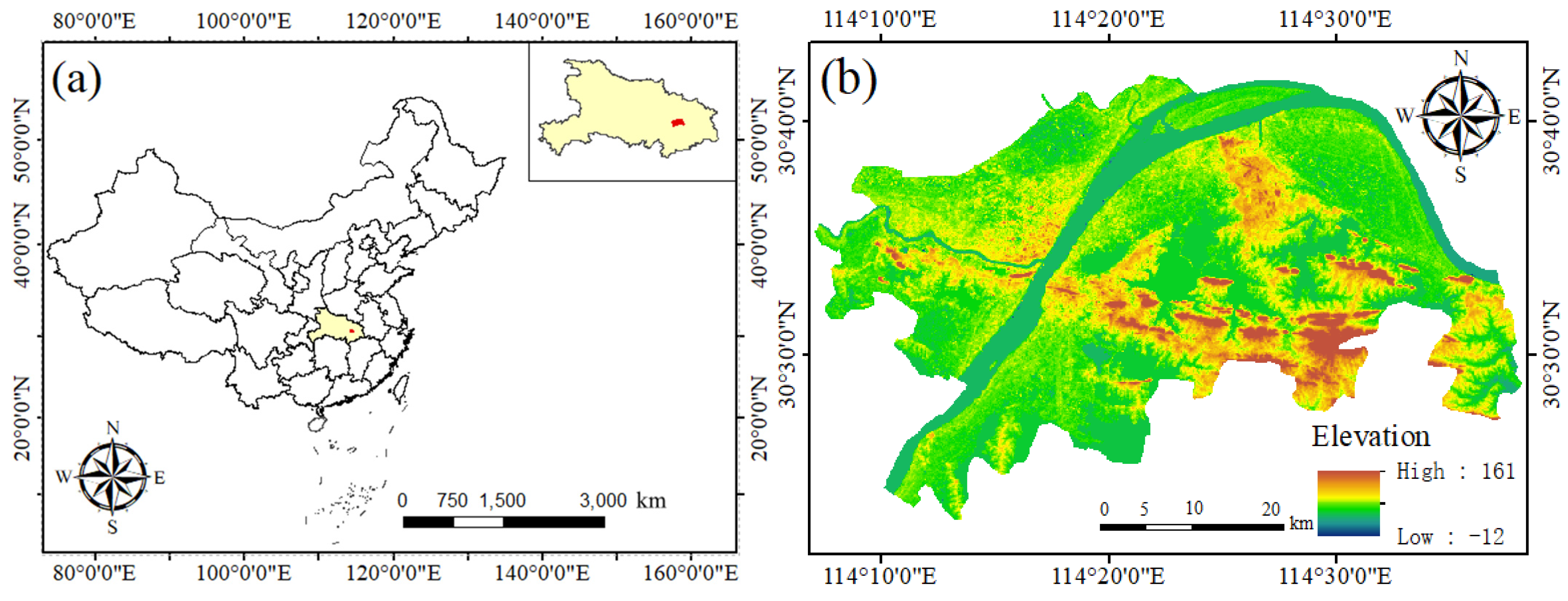
2.1. Study Area
2.2. Data Sources
3. Methods
3.1. LULC Classification
3.2. Accuracy of LULC Data
3.3. Inversion of Surface Temperature
3.4. The Prediction of LULC Map
3.5. The Prediction Process of LST
3.6. ANN Model
4. Results and Analysis
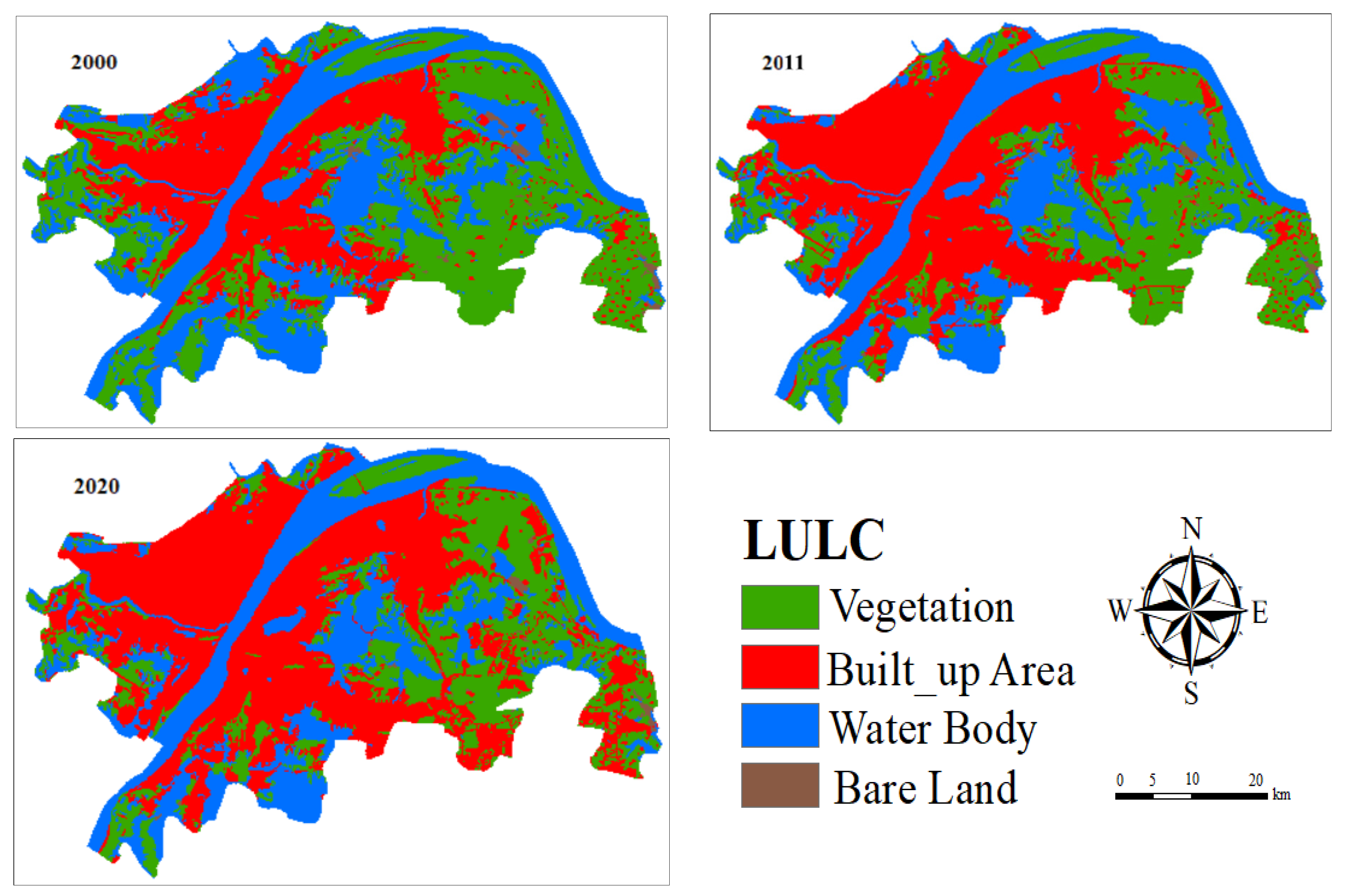
4.1. Variation in Past LULC Patterns
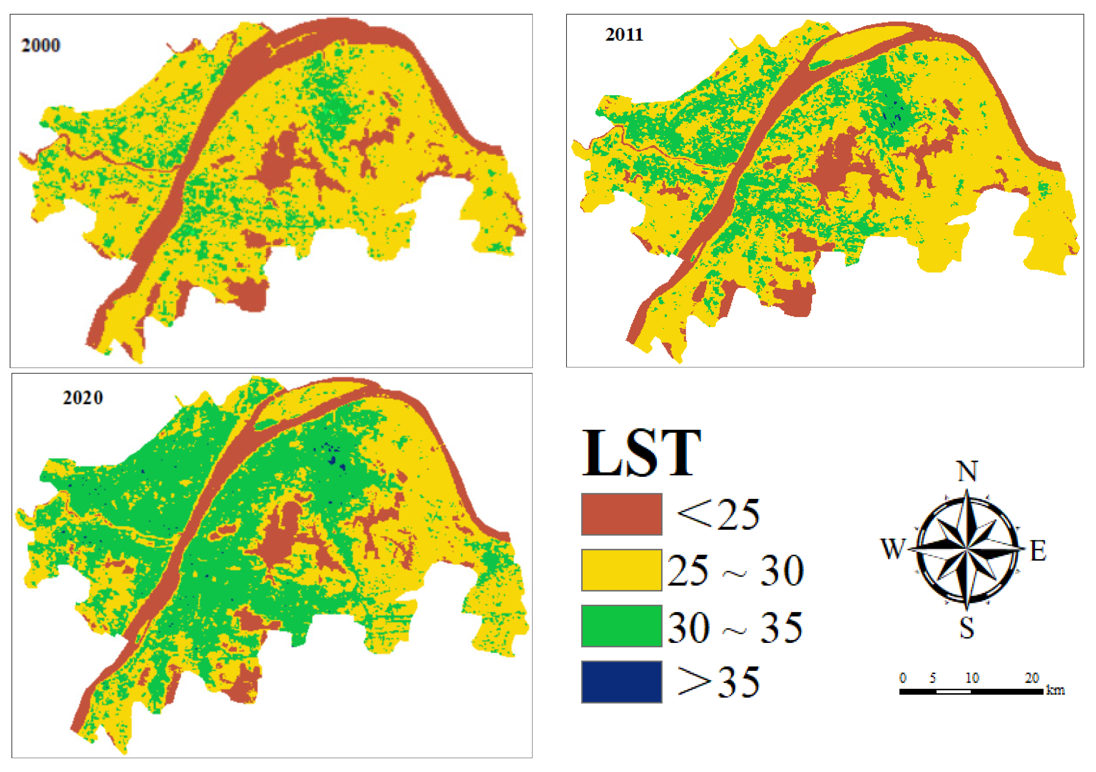
4.2. Analysis of LST Changes
4.3. Changes in LST under Different LULC
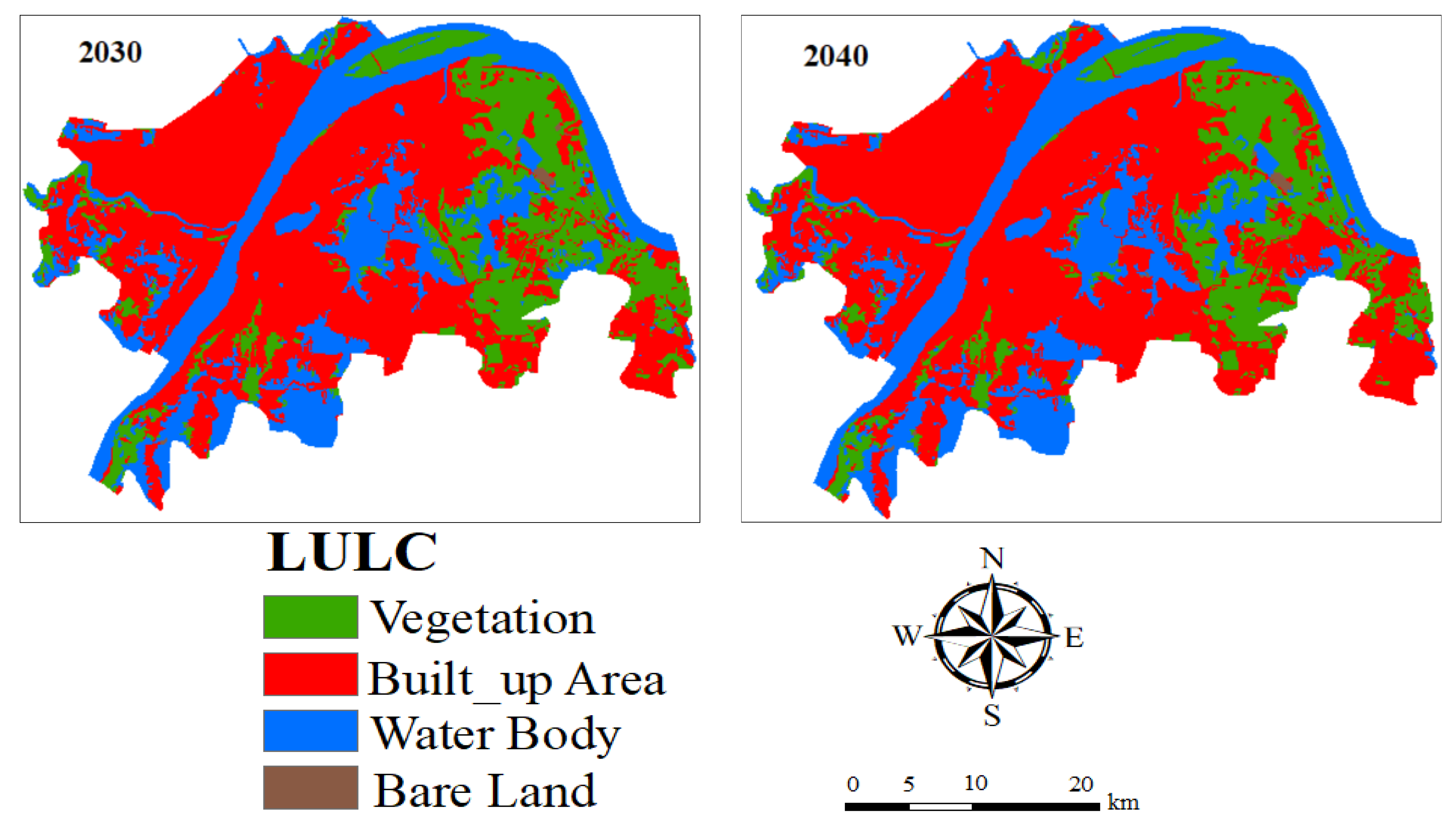
4.4. Prediction and Analysis of LULC
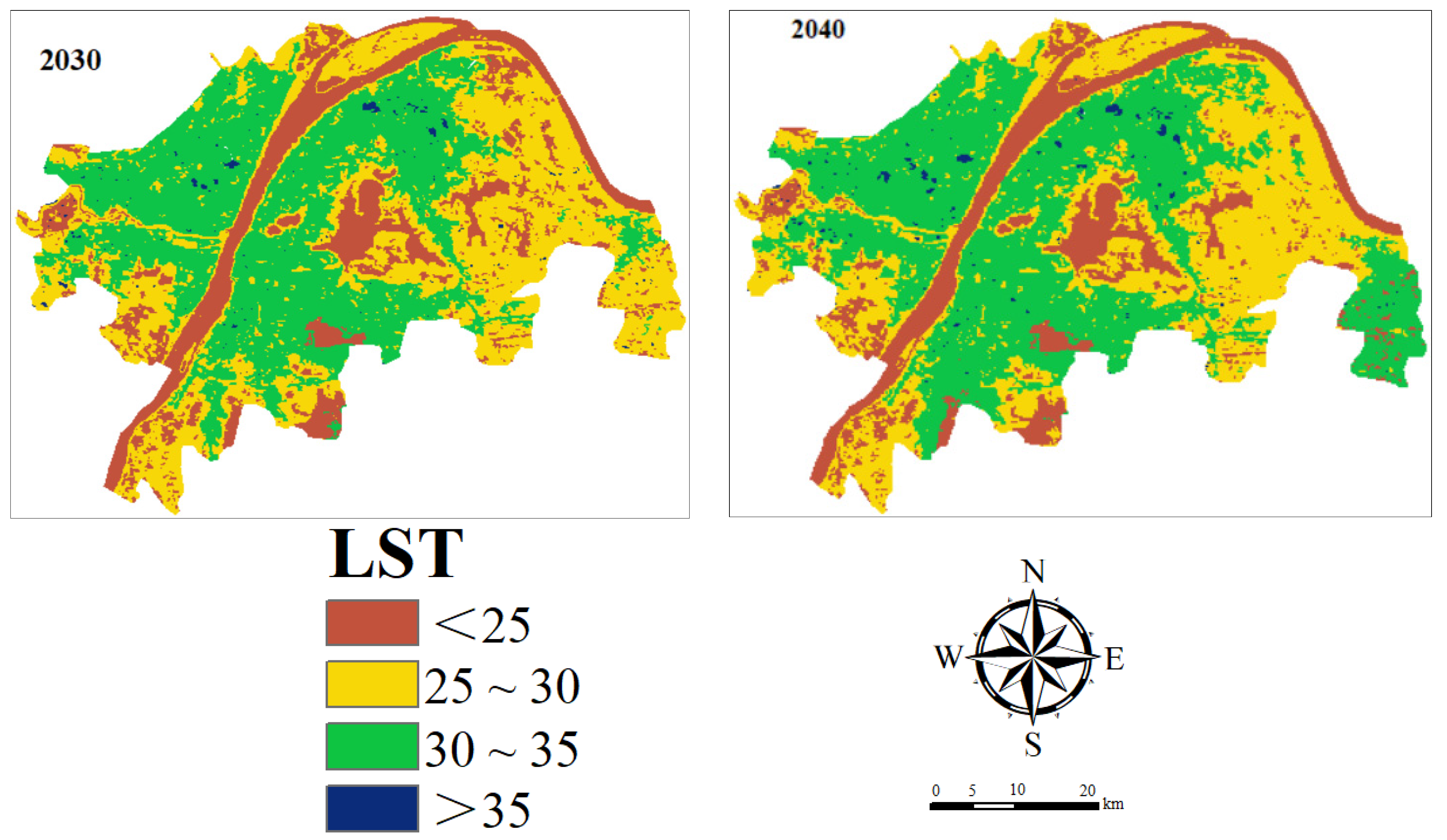
4.5. Prediction and Analysis of LST
5. Discussion and Conclusions
Author Contributions
Funding
Institutional Review Board Statement
Informed Consent Statement
Data Availability Statement
Acknowledgments
Conflicts of Interest
Appendix A
References
- Dong, F.; Zhang, S.; Long, R.; Zhang, X.; Sun, Z. Determinants of Haze Pollution: An Analysis from the Perspective of Spatiotemporal Heterogeneity. J. Clean. Prod. 2019, 222, 768–783. [Google Scholar] [CrossRef]
- Klemeš, J.J.; Fan, Y.V.; Tan, R.R.; Jiang, P. Minimising the Present and Future Plastic Waste, Energy and Environmental Footprints Related to COVID-19. Renew. Sustain. Energy Rev. 2020, 127, 109883. [Google Scholar] [CrossRef] [PubMed]
- Dong, L.; Tong, X.; Li, X.; Zhou, J.; Wang, S.; Liu, B. Some Developments and New Insights of Environmental Problems and Deep Mining Strategy for Cleaner Production in Mines. J. Clean. Prod. 2019, 210, 1562–1578. [Google Scholar] [CrossRef]
- Gu, C.; Guan, W.; Liu, H. Chinese Urbanization 2050: SD Modeling and Process Simulation. Sci. China Earth Sci. 2017, 60, 1067–1082. [Google Scholar] [CrossRef]
- Kalnay, E.; Cai, M. Impact of Urbanization and Land-Use Change on Climate. Nature 2003, 423, 528–531. [Google Scholar] [CrossRef]
- Cai, Z.; Liu, Q.; Cao, S. Real Estate Supports Rapid Development of China’s Urbanization. Land Use Policy 2020, 95, 104582. [Google Scholar] [CrossRef]
- Liu, F.; Zhang, X.; Murayama, Y.; Morimoto, T. Impacts of Land Cover/Use on the Urban Thermal Environment: A Comparative Study of 10 Megacities in China. Remote Sens. 2020, 12, 307. [Google Scholar] [CrossRef] [Green Version]
- George, M.; Pandey, A.K.; Abd Rahim, N.; Tyagi, V.V.; Shahabuddin, S.; Saidur, R. A Novel Polyaniline (PANI)/Paraffin Wax Nano Composite Phase Change Material: Superior Transition Heat Storage Capacity, Thermal Conductivity and Thermal Reliability. Sol. Energy 2020, 204, 448–458. [Google Scholar] [CrossRef]
- Rohde, D. Analysis of an Integrated Heating and Cooling System for a Building Complex with Focus on Long–Term Thermal Storage. Appl. Therm. Eng. 2018, 145, 13. [Google Scholar] [CrossRef]
- Chen, G.; Wang, D.; Wang, Q.; Li, Y.; Wang, X.; Hang, J.; Gao, P.; Ou, C.; Wang, K. Scaled Outdoor Experimental Studies of Urban Thermal Environment in Street Canyon Models with Various Aspect Ratios and Thermal Storage. Sci. Total Environ. 2020, 726, 138147. [Google Scholar] [CrossRef]
- Zhang, X.; Estoque, R.C.; Murayama, Y.; Ranagalage, M. Capturing Urban Heat Island Formation in a Subtropical City of China Based on Landsat Images: Implications for Sustainable Urban Development. Environ. Monit. Assess. 2021, 193, 130. [Google Scholar] [CrossRef] [PubMed]
- Li, H.; Zhou, Y.; Jia, G.; Zhao, K.; Dong, J. Quantifying the Response of Surface Urban Heat Island to Urbanization Using the Annual Temperature Cycle Model. Geosci. Front. 2021, 13, 101141. [Google Scholar] [CrossRef]
- Yu, Z.; Jing, Y.; Yang, G.; Sun, R. A New Urban Functional Zone-Based Climate Zoning System for Urban Temperature Study. Remote Sens. 2021, 13, 251. [Google Scholar] [CrossRef]
- Su, H.; Han, G.; Li, L.; Qin, H. The Impact of Macro-Scale Urban Form on Land Surface Temperature: An Empirical Study Based on Climate Zone, Urban Size and Industrial Structure in China. Sustain. Cities Soc. 2021, 74, 103217. [Google Scholar] [CrossRef]
- Taleghani, M.; Montazami, A.; Perrotti, D. Learning to Chill: The Role of Design Schools and Professional Training to Improve Urban Climate and Urban Metabolism. Energies 2020, 13, 2243. [Google Scholar] [CrossRef]
- Kwak, Y. Discerning the Success of Sustainable Planning—A Comparative Analysis of Urban Heat Island Dynamics in Korean New Towns. Sustain. Cities Soc. 2020, 61, 13. [Google Scholar] [CrossRef]
- Halder, B.; Bandyopadhyay, J.; Banik, P. Evaluation of the Climate Change Impact on Urban Heat Island Based on Land Surface Temperature and Geospatial Indicators. Int. J. Environ. Res. 2021, 15, 819–835. [Google Scholar] [CrossRef]
- Farrell, K.; Westlund, H. China’s Rapid Urban Ascent: An Examination into the Components of Urban Growth. Asian Geogr. 2018, 35, 85–106. [Google Scholar] [CrossRef] [Green Version]
- Guo, Y.; Han, J.; Zhao, X.; Dai, X.; Zhang, H. Understanding the Role of Optimized Land Use/Land Cover Components in Mitigating Summertime Intra-Surface Urban Heat Island Effect: A Study on Downtown Shanghai, China. Energies 2020, 13, 1678. [Google Scholar] [CrossRef] [Green Version]
- Kafy, A.-A.; Faisal, A.A.; Rahman, M.S.; Islam, M.; Al Rakib, A.; Islam, M.A.; Khan, M.H.H.; Sikdar, M.S.; Sarker, M.H.S.; Mawa, J.; et al. Prediction of Seasonal Urban Thermal Field Variance Index Using Machine Learning Algorithms in Cumilla, Bangladesh. Sustain. Cities Soc. 2021, 64, 102542. [Google Scholar] [CrossRef]
- Stewart, I.D. Why Should Urban Heat Island Researchers Study History? Urban Clim. 2019, 30, 100484. [Google Scholar] [CrossRef]
- Peng, X.; Wu, W.; Zheng, Y.; Sun, J.; Hu, T.; Wang, P. Correlation Analysis of Land Surface Temperature and Topographic Elements in Hangzhou, China. Sci. Rep. 2020, 10, 10451. [Google Scholar] [CrossRef] [PubMed]
- Li, H.; Wang, G.; Tian, G.; Jombach, S. Mapping and Analyzing the Park Cooling Effect on Urban Heat Island in an Expanding City: A Case Study in Zhengzhou City, China. Land 2020, 9, 57. [Google Scholar] [CrossRef] [Green Version]
- Ullah, S.; Ahmad, K.; Sajjad, R.U.; Abbasi, A.M.; Nazeer, A.; Tahir, A.A. Analysis and Simulation of Land Cover Changes and Their Impacts on Land Surface Temperature in a Lower Himalayan Region. J. Environ. Manag. 2019, 245, 348–357. [Google Scholar] [CrossRef] [PubMed]
- Goldblatt, R.; Addas, A.; Crull, D.; Maghrabi, A.; Levin, G.G.; Rubinyi, S. Remotely Sensed Derived Land Surface Temperature (LST) as a Proxy for Air Temperature and Thermal Comfort at a Small Geographical Scale. Land 2021, 10, 410. [Google Scholar] [CrossRef]
- Ma, X.; Peng, S. Assessing the Quantitative Relationships between the Impervious Surface Area and Surface Heat Island Effect during Urban Expansion. PeerJ 2021, 9, e11854. [Google Scholar] [CrossRef]
- Li, J.; Li, J.; Yuan, Y.; Li, G. Spatiotemporal Distribution Characteristics and Mechanism Analysis of Urban Population Density: A Case of Xi’an, Shaanxi, China. Cities 2019, 86, 62–70. [Google Scholar] [CrossRef]
- Amindin, A.; Pouyan, S.; Pourghasemi, H.R.; Yousefi, S.; Tiefenbacher, J.P. Spatial and Temporal Analysis of Urban Heat Island Using Landsat Satellite Images. Environ. Sci. Pollut. Res. 2021, 28, 41439–41450. [Google Scholar] [CrossRef]
- Abdelhaleem, F.S. Application of Remote Sensing and Geographic Information Systems in Irrigation Water Management under Water Scarcity Conditions in Fayoum, Egypt. J. Environ. Manag. 2021, 299, 9. [Google Scholar] [CrossRef] [PubMed]
- Ouma, Y.O.; Okuku, C.O.; Njau, E.N. Use of Artificial Neural Networks and Multiple Linear Regression Model for the Prediction of Dissolved Oxygen in Rivers: Case Study of Hydrographic Basin of River Nyando, Kenya. Complexity 2020, 2020, 1–23. [Google Scholar] [CrossRef]
- Kafy, A.-A.; Naim, M.N.H.; Subramanyam, G.; Faisal, A.-A.; Ahmed, N.U.; Rakib, A.A.; Kona, M.A.; Sattar, G.S. Cellular Automata Approach in Dynamic Modelling of Land Cover Changes Using RapidEye Images in Dhaka, Bangladesh. Environ. Chall. 2021, 4, 100084. [Google Scholar] [CrossRef]
- Siddiqui, A.; Siddiqui, A.; Maithani, S.; Jha, A.K.; Kumar, P.; Srivastav, S.K. Urban Growth Dynamics of an Indian Metropolitan Using CA Markov and Logistic Regression. Egypt. J. Remote Sens. Space Sci. 2018, 21, 229–236. [Google Scholar] [CrossRef]
- Porte, X.; Skalli, A.; Haghighi, N.; Reitzenstein, S.; Lott, J.A.; Brunner, D. A Complete, Parallel and Autonomous Photonic Neural Network in a Semiconductor Multimode Laser. J. Phys. Photonics 2021, 3, 9. [Google Scholar] [CrossRef]
- Noori, N.; Kalin, L.; Isik, S. Water Quality Prediction Using SWAT-ANN Coupled Approach. J. Hydrol. 2020, 590, 125220. [Google Scholar] [CrossRef]
- Qin, Z.; Karnieli, A.; Berliner, P. A mono-window algorithm for retrieving land surface temperature from Landsat TM data and its application to the Israel-Egypt border region. Int. J. Remote Sens. 2001, 22, 3719–3746. [Google Scholar] [CrossRef]
- Wang, M.; Wan, Y.; Ye, Z.; Lai, X. Remote Sensing Image Classification Based on the Optimal Support Vector Machine and Modified Binary Coded Ant Colony Optimization Algorithm. Inf. Sci. 2017, 402, 50–68. [Google Scholar] [CrossRef]
- Mishra, V.N.; Prasad, R.; Rai, P.K.; Vishwakarma, A.K.; Arora, A. Performance Evaluation of Textural Features in Improving Land Use/Land Cover Classification Accuracy of Heterogeneous Landscape Using Multi-Sensor Remote Sensing Data. Earth Sci. Inform. 2019, 12, 71–86. [Google Scholar] [CrossRef]
- Sekertekin, A.; Bonafoni, S. Land Surface Temperature Retrieval from Landsat 5, 7, and 8 over Rural Areas: Assessment of Different Retrieval Algorithms and Emissivity Models and Toolbox Implementation. Remote Sens. 2020, 12, 294. [Google Scholar] [CrossRef] [Green Version]
- Naim, M.N.H.; Kafy, A.-A. Assessment of Urban Thermal Field Variance Index and Defining the Relationship between Land Cover and Surface Temperature in Chattogram City: A Remote Sensing and Statistical Approach. Environ. Chall. 2021, 4, 100107. [Google Scholar] [CrossRef]
- Ahmad, T.B.; Liu, L.; Kotiw, M.; Benkendorff, K. Review of Anti-Inflammatory, Immune-Modulatory and Wound Healing Properties of Molluscs. J. Ethnopharmacol. 2018, 210, 156–178. [Google Scholar] [CrossRef]
- Lai, L.-W.; Cheng, W.-L. 0> Urban Heat Island and Air Pollution—An Emerging Role for Hospital Respiratory Admissions in an Urban Area. J. Environ. Health 2010, 72, 32–36. [Google Scholar] [PubMed]
- Santé, I.; García, A.M.; Miranda, D.; Crecente, R. Cellular Automata Models for the Simulation of Real-World Urban Processes: A Review and Analysis. Landsc. Urban Plan. 2010, 96, 108–122. [Google Scholar] [CrossRef]
- Luo, Y.; Sun, W.; Yang, K.; Zhao, L. China Urbanization Process Induced Vegetation Degradation and Improvement in Recent 20 Years. Cities 2021, 114, 103207. [Google Scholar] [CrossRef]
- Liu, L.; Zhang, Y. Urban Heat Island Analysis Using the Landsat TM Data and ASTER Data: A Case Study in Hong Kong. Remote Sens. 2011, 3, 1535–1552. [Google Scholar] [CrossRef] [Green Version]
- Yang, J.; Ren, J.; Sun, D.; Xiao, X.; Xia, J.C.; Jin, C.; Li, X. Understanding Land Surface Temperature Impact Factors Based on Local Climate Zones. Sustain. Cities Soc. 2021, 69, 102818. [Google Scholar] [CrossRef]
- Hanberry, B.B. Timing of Tree Density Increases, Influence of Climate Change, and a Land Use Proxy for Tree Density Increases in the Eastern United States. Land 2021, 10, 1121. [Google Scholar] [CrossRef]
- Koko, A.F.; Wu, Y.; Abubakar, G.A.; Alabsi, A.A.N.; Hamed, R.; Bello, M. Thirty Years of Land Use/Land Cover Changes and Their Impact on Urban Climate: A Study of Kano Metropolis, Nigeria. Land 2021, 10, 1106. [Google Scholar] [CrossRef]
- Sejati, A.W.; Buchori, I.; Rudiarto, I. The Spatio-Temporal Trends of Urban Growth and Surface Urban Heat Islands over Two Decades in the Semarang Metropolitan Region. Sustain. Cities Soc. 2019, 46, 101432. [Google Scholar] [CrossRef]
- Yu, Z.; Yang, K.; Luo, Y.; Shang, C. Spatial-Temporal Process Simulation and Prediction of Chlorophyll-a Concentration in Dianchi Lake Based on Wavelet Analysis and Long-Short Term Memory Network. J. Hydrol. 2020, 582, 124488. [Google Scholar] [CrossRef]
- Zhao, Z.; Sharifi, A.; Dong, X.; Shen, L.; He, B.-J. Spatial Variability and Temporal Heterogeneity of Surface Urban Heat Island Patterns and the Suitability of Local Climate Zones for Land Surface Temperature Characterization. Remote Sens. 2021, 13, 4338. [Google Scholar] [CrossRef]
- Ullah, S.; Tahir, A.A.; Akbar, T.A.; Hassan, Q.K.; Dewan, A.; Khan, A.J.; Khan, M. Remote Sensing-Based Quantification of the Relationships between Land Use Land Cover Changes and Surface Temperature over the Lower Himalayan Region. Sustainability 2019, 11, 5492. [Google Scholar] [CrossRef] [Green Version]
- Santamouris, M. Recent Progress on Urban Overheating and Heat Island Research. Integrated Assessment of the Energy, Environmental, Vulnerability and Health Impact. Synergies with the Global Climate Change. Energy Build. 2020, 207, 109482. [Google Scholar] [CrossRef]
- Yang, J.; Wang, Y.; Xiu, C.; Xiao, X.; Xia, J.; Jin, C. Optimizing Local Climate Zones to Mitigate Urban Heat Island Effect in Human Settlements. J. Clean. Prod. 2020, 275, 123767. [Google Scholar] [CrossRef]
- Mansour, S.; Al-Belushi, M.; Al-Awadhi, T. Monitoring Land Use and Land Cover Changes in the Mountainous Cities of Oman Using GIS and CA-Markov Modelling Techniques. Land Use Policy 2020, 91, 104414. [Google Scholar] [CrossRef]
- He, B.-J.; Wang, J.; Liu, H.; Ulpiani, G. Localized Synergies between Heat Waves and Urban Heat Islands: Implications on Human Thermal Comfort and Urban Heat Management. Environ. Res. 2021, 193, 110584. [Google Scholar] [CrossRef]
- Lo, C.P.; Quattrochi, D.A. Land-Use and Land-Cover Change, Urban Heat Island Phenomenon, and Health Implications. Photogramm. Eng. Remote Sens. 2003, 69, 1053–1063. [Google Scholar] [CrossRef]
- Yu, X.; Guo, X.; Wu, Z. Land Surface Temperature Retrieval from Landsat 8 TIRS—Comparison between Radiative Transfer Equation-Based Method, Split Window Algorithm and Single Channel Method. Remote Sens. 2014, 6, 9829–9852. [Google Scholar] [CrossRef] [Green Version]
- Talukdar, S.; Rihan, M.; Hang, H.T.; Bhaskaran, S.; Rahman, A. Modelling Urban Heat Island (UHI) and Thermal Field Variation and Their Relationship with Land Use Indices over Delhi and Mumbai Metro Cities. Environ. Dev. Sustain. 2021, 21, 1–29. [Google Scholar] [CrossRef]
- dos Santos, A.R.; de Oliveira, F.S.; da Silva, A.G.; Gleriani, J.M.; Gonçalves, W.; Moreira, G.L.; Silva, F.G.; Branco, E.R.F.; Moura, M.M.; da Silva, R.G.; et al. Spatial and Temporal Distribution of Urban Heat Islands. Sci. Total Environ. 2017, 605–606, 946–956. [Google Scholar] [CrossRef]


| Date of Acquisition | Sensor | Path/Row | Multi-Spectral Band Resolution | Cloud Cover |
|---|---|---|---|---|
| 27 July 2000 | TM | 123/39 | 30 m | <10% |
| 8 June 2011 | TM | 123/39 | 30 m | <10% |
| 3 August 2020 | OLI_TIRS | 123/39 | 30 m | <10% |
| Year | User Accuracy (%) | Producer Accuracy (%) | Overrall Accuracy (%) | Kappa Statistics (%) |
|---|---|---|---|---|
| 2000 | 87.56 | 89.51 | 98.12 | 89.68 |
| 2011 | 89.16 | 90.33 | 87.97 | 91.25 |
| 2020 | 91.08 | 88.24 | 91.37 | 90.18 |
| Class | 2000 | 2011 | 2020 | 2000–2020 | |
|---|---|---|---|---|---|
| Area (Km2) | Area of Change (Km2) | Rate of Change (%) | |||
| Vegetation | 370.675 | 283.554 | 246.859 | −123.816 | −50.16 |
| Built-Up Area | 267.683 | 388.852 | 452.111 | 184.428 | 40.79 |
| Water Body | 320.742 | 289.869 | 263.898 | −56.844 | −21.54 |
| Bare Land | 8.365 | 5.192 | 4.599 | −3.766 | −81.88 |
| Year | <25 °C | 25~30 °C | 30~35 °C | >35 °C | ||||
|---|---|---|---|---|---|---|---|---|
| Area | Ratio | Area | Ratio | Area | Ratio | Area | Ratio | |
| (Km2) | (%) | (Km2) | (%) | (Km2) | (%) | (Km2) | (%) | |
| 2000 | 152.015 | 15.713 | 501.872 | 51.874 | 313.581 | 32.413 | 0 | 0 |
| 2011 | 139.273 | 14.396 | 398.596 | 41.200 | 423.066 | 43.729 | 6.533 | 0.675 |
| 2020 | 126.448 | 13.069 | 315.661 | 32.627 | 515.108 | 53.242 | 10.251 | 1.059 |
| LULC | <25 °C | 25~30 °C | 30~35 °C | >35 °C | ||||
|---|---|---|---|---|---|---|---|---|
| Area (Km2) | Ratio (%) | Area (Km2) | Ratio (%) | Area (Km2) | Ratio (%) | Area (Km2) | Ratio (%) | |
| 2000 | ||||||||
| Vegetation | 33.214 | 3.433 | 183.474 | 18.964 | 153.987 | 15.917 | 0.000 | 0.000 |
| Built-up Area | 11.435 | 1.182 | 114.847 | 11.871 | 141.401 | 14.616 | 0.000 | 0.000 |
| Water Body | 105.413 | 10.896 | 199.106 | 20.580 | 16.254 | 1.680 | 0.000 | 0.000 |
| Bare Land | 1.953 | 0.202 | 4.445 | 0.459 | 1.967 | 0.203 | 0.000 | 0.000 |
| 2011 | ||||||||
| Vegetation | 30.521 | 3.155 | 161.651 | 16.709 | 90.757 | 9.381 | 0.817 | 0.084 |
| Built-up Area | 5.120 | 0.529 | 80.276 | 8.298 | 299.307 | 30.937 | 3.978 | 0.411 |
| Water Body | 103.554 | 10.704 | 153.924 | 15.910 | 32.361 | 3.345 | 0.013 | 0.001 |
| Bare Land | 0.078 | 0.008 | 2.765 | 0.286 | 0.641 | 0.066 | 1.708 | 0.177 |
| 2020 | ||||||||
| Vegetation | 32.321 | 3.341 | 114.685 | 11.854 | 99.057 | 10.239 | 0.915 | 0.095 |
| Built-up Area | 6.921 | 0.715 | 85.258 | 8.812 | 354.149 | 36.606 | 5.783 | 0.598 |
| Water Body | 86.244 | 8.914 | 112.779 | 11.657 | 61.785 | 6.386 | 3.058 | 0.316 |
| Bare Land | 0.962 | 0.099 | 2.894 | 0.299 | 0.241 | 0.025 | 0.502 | 0.052 |
| LULC Class | Area(Km2) | Net Change (%) | |||||
|---|---|---|---|---|---|---|---|
| 2000 | 2011 | 2020 | 2030 | 2040 | 2020~2030 | 2020~2040 | |
| Vegetation | 370.6749 | 283.554 | 246.859 | 200.559 | 185.687 | −18.76 | −24.78 |
| Built-up Area | 267.6834 | 388.8522 | 452.111 | 511.51 | 545.282 | 13.14 | 20.61 |
| Water Body | 320.742 | 289.8693 | 263.898 | 253.267 | 234.616 | −4.03 | −11.10 |
| Bare Land | 8.3646 | 5.1921 | 4.599 | 2.13 | 1.881 | −53.28 | −58.74 |
| Year | <25 °C | 25~30 °C | 30~35 °C | >35 °C | ||||
|---|---|---|---|---|---|---|---|---|
| Area | Ratio | Area | Ratio | Area | Ratio | Area | Ratio | |
| (Km2) | (%) | (Km2) | (%) | (Km2) | (%) | (Km2) | (%) | |
| 2030 | 121.257 | 12.533 | 318.915 | 32.964 | 512.032 | 52.925 | 15.264 | 1.578 |
| 2040 | 98.544 | 10.186 | 301. 097 | 31.122 | 534.215 | 55.219 | 33.612 | 3.473 |
Publisher’s Note: MDPI stays neutral with regard to jurisdictional claims in published maps and institutional affiliations. |
© 2021 by the authors. Licensee MDPI, Basel, Switzerland. This article is an open access article distributed under the terms and conditions of the Creative Commons Attribution (CC BY) license (https://creativecommons.org/licenses/by/4.0/).
Share and Cite
Zhang, M.; Zhang, C.; Kafy, A.-A.; Tan, S. Simulating the Relationship between Land Use/Cover Change and Urban Thermal Environment Using Machine Learning Algorithms in Wuhan City, China. Land 2022, 11, 14. https://0-doi-org.brum.beds.ac.uk/10.3390/land11010014
Zhang M, Zhang C, Kafy A-A, Tan S. Simulating the Relationship between Land Use/Cover Change and Urban Thermal Environment Using Machine Learning Algorithms in Wuhan City, China. Land. 2022; 11(1):14. https://0-doi-org.brum.beds.ac.uk/10.3390/land11010014
Chicago/Turabian StyleZhang, Maomao, Cheng Zhang, Abdulla-Al Kafy, and Shukui Tan. 2022. "Simulating the Relationship between Land Use/Cover Change and Urban Thermal Environment Using Machine Learning Algorithms in Wuhan City, China" Land 11, no. 1: 14. https://0-doi-org.brum.beds.ac.uk/10.3390/land11010014