
Competition between Export Cities in China: Evolution and Influencing Factors

1
School of Architectural Engineering, Jinling Institute of Technology, Nanjing 211169, China
2
School of Geography Science, Nanjing Normal University, Nanjing 210023, China
3
School of International Economics and Trade, Nanjing University of Finance and Economics, Nanjing 210023, China
*
Author to whom correspondence should be addressed.
Land 2022, 11(2), 201; https://0-doi-org.brum.beds.ac.uk/10.3390/land11020201
Submission received: 25 December 2021
/
Revised: 19 January 2022
/
Accepted: 26 January 2022
/
Published: 28 January 2022
Abstract
:Based on the Export Similarity Index (ESI), this study examines the export competition pattern among Chinese cities in the global market from 2000 to 2017, analyzing the mechanism of competition using a panel Granger causality test and a gravity model. The study reports several findings, as follows: (1) The competition pattern among Chinese cities first increased and then decreased, and the ESI between most cities was low. (2) More provincial capitals in the central and western regions converged with the developed eastern regions in their export structures, and cities in the regions of Beijing-Tianjin-Hebei, Yangtze River Delta, and Pearl River Delta competed differently. (3) Using all cities in the sample, the results show a bidirectional causal relationship between a city’s Gross Domestic Product (GDP) and the average export competitive pressure from other cities. However, results for the provincial capitals and three urban agglomerations indicated that GDP intensifies competition among cities. (4) The gravity model’s regression results show that the larger the economic size and the smaller the distance between cities, the more obvious the competition between them. This study provides a new direction for the study of export trade from the perspective of urban scale.
1. Introduction
Export trade is an important driving force behind urban development in China [1]. Chinese cities at different stages of development and on different bases of development vary in the types and quality of goods they export to other countries, while also competing with each other [2]. For example, radio equipment made up 15.22% and 14.41% of the goods exported by Shenzhen and Dongguan, respectively, in 2017. Shenzhen and Dongguan are located in close proximity, and both have developed economies in the Pearl River Delta (PRD). As in their case, similar export structures often lead to fierce competition between cities.
In China, a country experiencing rapid urbanization and industrialization [3,4], the competition between export cities is also complex and changing. Analyzing this kind of competitive relationship will provide a scientific basis for the government to produce development plans and industrial layouts. In fact, under the tide of informatization and globalization, cities gradually became the “rational economic man” in a geographical space. To compete with other cities in the world trade market is a challenge that must be faced in the process of urban development. The analysis of this evolution process and the internal mechanisms of this competitive relationship will also help cities consider their own economic and geographic environments more scientifically when constructing export strategies.
So, what is the competitive pattern of export trade among Chinese cities? In some typical urban agglomeration areas, what are the characteristics of this competition? What are the underlying causes of this competitive pattern? We will focus on exploring these issues. The paper is structured as follows: Section 1.1 presents a critical review of the literature on competition between export countries and identifies the lack of research on export competition at the city level and the lack of a network analysis perspective. Section 1.2 describes the hypothesis and framework. Section 2 presents the methodology, data, and study area. Section 3 reports and discusses the results of the analysis, and Section 4 discusses the conclusions and the implications of the study findings.
1.1. Literature Review: Competition between Export Countries
Existing research on the competition between different regions in trade markets mainly focuses on countries. Some studies focus on European countries, especially on export competition among countries within the European Union [5,6]. There are also studies focusing on export competition between EU countries and other regions [7,8,9]. From the perspective of structural change, they discuss the development history of EU trade before and after the eastern expansion of the EU.
When scholars discuss export trade competition among European countries, they seldom analyze the economic and geographical factors that produce the competition relationship—in particular, whether factors such as economic size and stage of development affect the competitive pressure a country faces in the global market. However, the analysis of this problem has been well addressed in other research regions: some scholars have seriously and rigorously analyzed the dynamic mechanism of China’s export trade competition with other countries. Both Dean et al. and Schott’s analyses of the internal causes of the export competition between China and other countries show that the larger China’s economic aggregate is, the more intense the trade competition between China and other countries will be [10,11]. In addition, the improvement in human capital and the government policies in the form of tax-favored high-tech zones also explain China’s export structure evolution [12].
In fact, the export trade competition between China and other countries (regions) has become a popular topic in academic circles in the past decade. Studies have identified different competition relations between China and Latin American countries [13], China and OECD countries [14,15], and China and ASEAN countries [16] in different years. Most of these studies agree that China’s rapid trade growth brought some challenges and pressures to other countries. These studies also reflect China’s increasingly sophisticated export structure, which is closer to that of the developed world, as China’s economy grows.
In the literature on the export trade competition among the countries mentioned above, Finger’s Export Similarity Index (ESI) is a key index used to calculate the size of the competitive relationship between two countries [17]. The ESI can indicate the degree of convergence of the commodities of two regions in a certain market. The higher the ESI, the more intense the competitive relationship.
Extant studies on the competitive relationship of export trade using ESI mostly focus on relationships between countries, with little discussion of the competitive export trade relationship between cities. Additionally, competition is a kind of relationship, and relationships can “connect” different regions. These interlinked relationships will form a network. However, the existing research on competitive relationships of export trade rarely uses network analysis. Only a few studies used network analysis when analyzing the export competition between countries [18,19]. Taking Chinese cities as its research object, this paper discusses the evolution and mechanism of the competition between cities in the global export market from 2000 to 2017. By doing so, this paper not only expands the study of export competition relations at a city scale, but also makes a comparative analysis of the competition relations among cities in different urban agglomerations in China, with certain policy implications for the cities’ foreign economic development.
1.2. Hypothesis and Framework: Competition between Export Cities
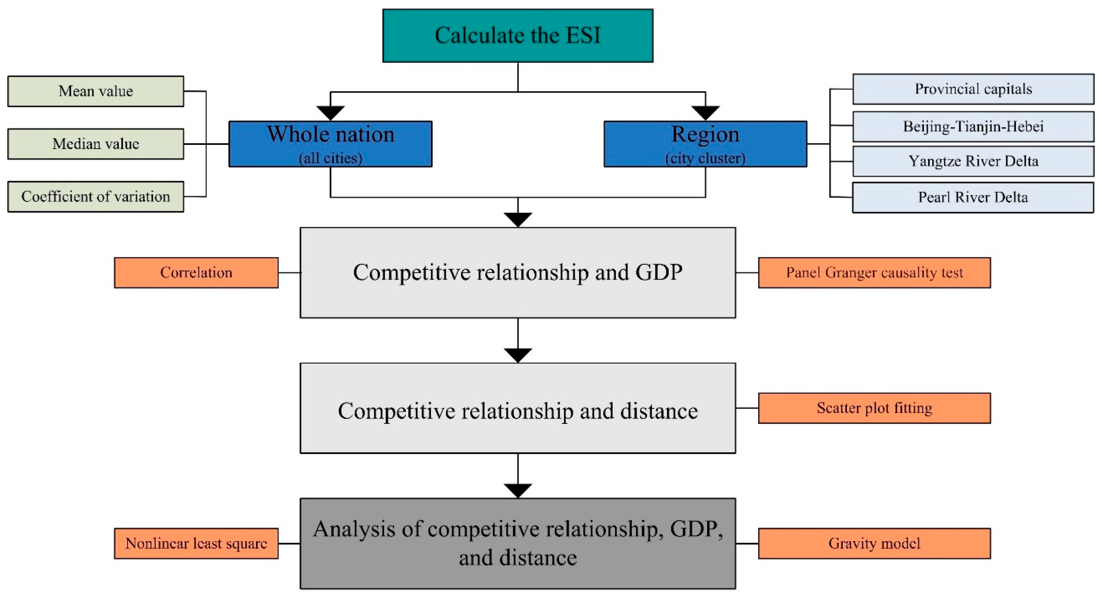
Based on the above discussion, we propose that there is a competitive relationship between Chinese cities in export trade and, furthermore, that this competitive relationship is different in different regions. To verify these hypotheses and further analyze the internal mechanism behind the competitive relationship, we adopt the following research framework (see Figure 1):
- The ESI is used to represent the export competition between cities, and the evolution of the ESIs from all cities and regions is analyzed to form an overall understanding of the competitive relationships among cities.
- The panel Granger causality test model is used to analyze the relationship between export competitive relationships and Gross Domestic Product (GDP).
- The relationship between export competitive relationships and geographical distance is explored through scatter plot fitting.
- The mechanism of the evolution of export competitive relationships between cities is explored by using the nonlinear least square (NLS) method, based on the gravity model.
2. Materials and Methods
2.1. Methodology
2.1.1. ESI and Average Export Similarity Index (AESI)
Many scholars, especially those who focus on economic geography, adopted the ESI to reflect the similarity in exports between regions in studies related to international trade, industrial economies, and other multidisciplinary fields [17,20,21]. The formula is as follows:
where is the similarity between city and city regarding the exports in market , represents the ratio of the commodity exported by city to market to the total exports of city to market , and represents the ratio of the commodity exported by city to market to the total exports of city to market . The value of is between 0 and 100, and the closer it is to 100, the more similar the export products of city and city in market are. In short, the higher is, the more intense the export competition between city and city is; the lower is, the less intense the export competition between city and city is. In this article, market is the global market.
The ESI represents the relationship between two cities. To investigate the overall competition between each city with other cities in the global market, we introduce a new indicator, the AESI, which we calculate as:
This study’s research object is 270 cities. Each city will have one ESI with every other city, which means each city will have 269 ESIs. The higher the , the greater the competitive pressure city faces from other cities in the global market.
2.1.2. Panel Unit Root Tests
Previous studies used panel unit root tests over normal time series unit root tests as they have superior power [22]. Based on previous studies [23,24,25], we adopted the Levin-Lin-Chu (LLC) test created by Levin et al. using Stata/MP 16.0 [26]. The formula is:
where is the panel data, is a unit of the cross-section, is time, is the common autoregression coefficient, is the panel-specific mean, is the coefficient, is the lag order, and is the error term.
2.1.3. Panel Cointegration Tests
While many panel cointegration techniques exist, such as those by Kao [27] and Pedroni [28], we utilized Westerlund’s cointegration method to test the cointegrating relationships between the variables [29]. The formula is
where represents the trend effects, represents the deterministic components, and is the error correction parameter. The remaining parameters have the same meanings as in Formula (3).
2.1.4. Panel Granger Causality Test
As an important means of causal analysis used by scholars in the field of econometrics, the Granger causality test is widely used in the study of many aspects of human and economic geography, such as urbanization [30] and international trade [31]. This model was first proposed by Granger [32]. Subsequently, Dumitrescu and Hurlin proposed a test based on panel data, which further promoted the application of this model in the field of econometrics [33]. Compared with the simple causal analysis of a time series, the panel Granger causality test provides an important method for researchers to examine the inherent nature of data in multiple dimensions. The formula is
where and are the independent and dependent variables, respectively, at the observation point , is the lag order, and are coefficients, and is the error term. The panel Granger causality test assumes that the past value of does not help predict the future value of as the null hypothesis (). If the result is the rejection of , then is said to be the Granger cause of .
In the panel Granger causality analysis, the choice of the lag order is key. Thanks to the development of measurement methods on Stata/MP 16.0, we were able to determine the optimal lag order under three different criteria (Akaike’s Information Criterion—AIC [34], Bayesian Information Criterion—BIC [35], and Hannan and Quinn’s Information Criterion—HQIC [36]) by using the xtgcause command.
2.1.5. Gravity Model
As the core theory of classical physics, gravity models were gradually introduced to many disciplines including economics [37], transport geography [38], economic geography [39], and urban and regional planning [40,41,42] by humanities and social sciences scholars. The formula is
where is the strength of connection between regions and , which can be traffic flow, population flow, trade flow, and so on. In addition, can represent relationships. and are the “qualities” of regions and , such as their GDP, GNP, and population. is the geographical distance between regions and , and and are parameters.
2.2. Data and Study Area
2.2.1. Data
The data (2000–2017) in this study were taken from two sources:
- The export data of each city came from the customs database of China (service trade data are not included). According to the enterprise codes, the export situation of enterprises in the same cities were summarized and used as the original export data of those cities. In addition, the customs database includes a large span of data collection years, resulting in multiple versions (HS1996, HS2002, HS2007, HS2012, and HS2017). Although the differences between the versions are not significant from a macro viewpoint, each version has a certain degree of fine-tuning compared with its previous version, so they need to be recoded systematically. According to the comparison table of the commodity codes issued by the United Nations Trade Database (https://unstats.un.org/unsd/trade/classifications/correspondence-tables.asp (accessed on 1 June 2021)), we uniformly adjusted the 8-digit commodity codes of every year of the customs data to the HS1996 version with 6-digit codes, so that the export similarity between the different years could be comparatively measured. However, because of the large amount of data in the customs database, there were extremely large calculation tasks when determining the ESI between different cities in different years. Therefore, we used PyCharm to calculate the ESIs programmatically.
- In addition to the data processing of the customs database, the GDP for each city in this study was taken from the cities’ statistical yearbooks and the provincial statistical yearbooks. Data that were difficult to obtain for some regions and years were based on the National Economic and Social Development Statistical Bulletin and local yearbooks.
2.2.2. Study Area
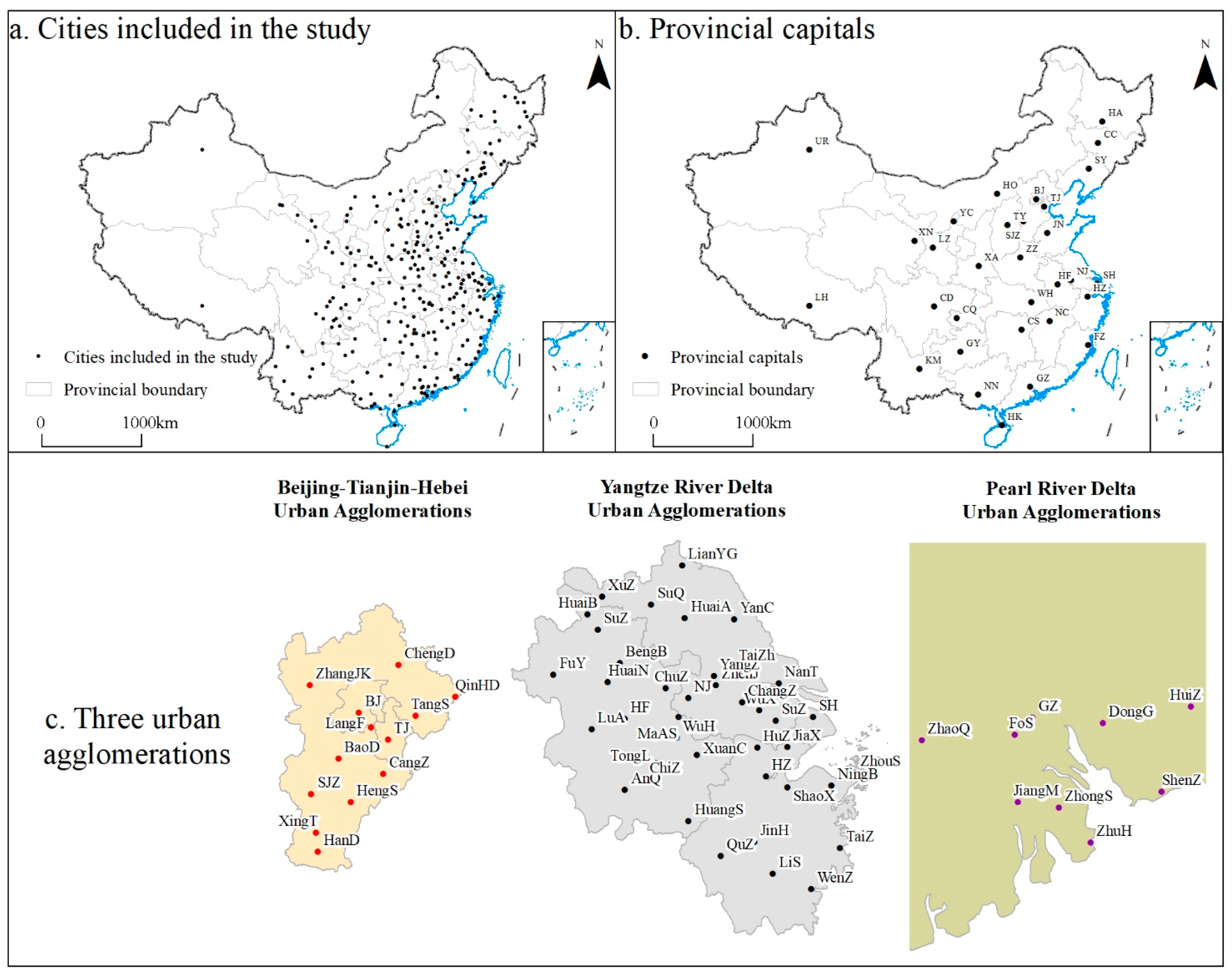
After synthesizing the availability of all data, we selected 270 cities as the analysis objects (see Figure 2a). To analyze the export competition situation of all cities in the global market, it is necessary to consider the overall situation at a macro-scale as well as to analyze local aspects to explore the temporal and spatial evolution characteristics of the export similarities between cities in different regions. Therefore, we focus on the analysis of provincial capitals and China’s three coastal urban agglomerations (see Figure 2b,c). The provincial capitals are the economic centers of the provinces, with high levels of industrialization and strong export capacity. Beijing–Tianjin–Hebei (BTH), Yangtze River Delta (YRD), and PRD play a crucial role in China’s export trade as the three most mature and economically active urban agglomerations in China.1 In 2017, the export volume of these three urban agglomerations reached USD 1,598 billion, accounting for 70.60% of China’s total export volume.
3. Results and Discussion
3.1. Spatiotemporal Evolution of the ESI
3.1.1. Overall Analysis
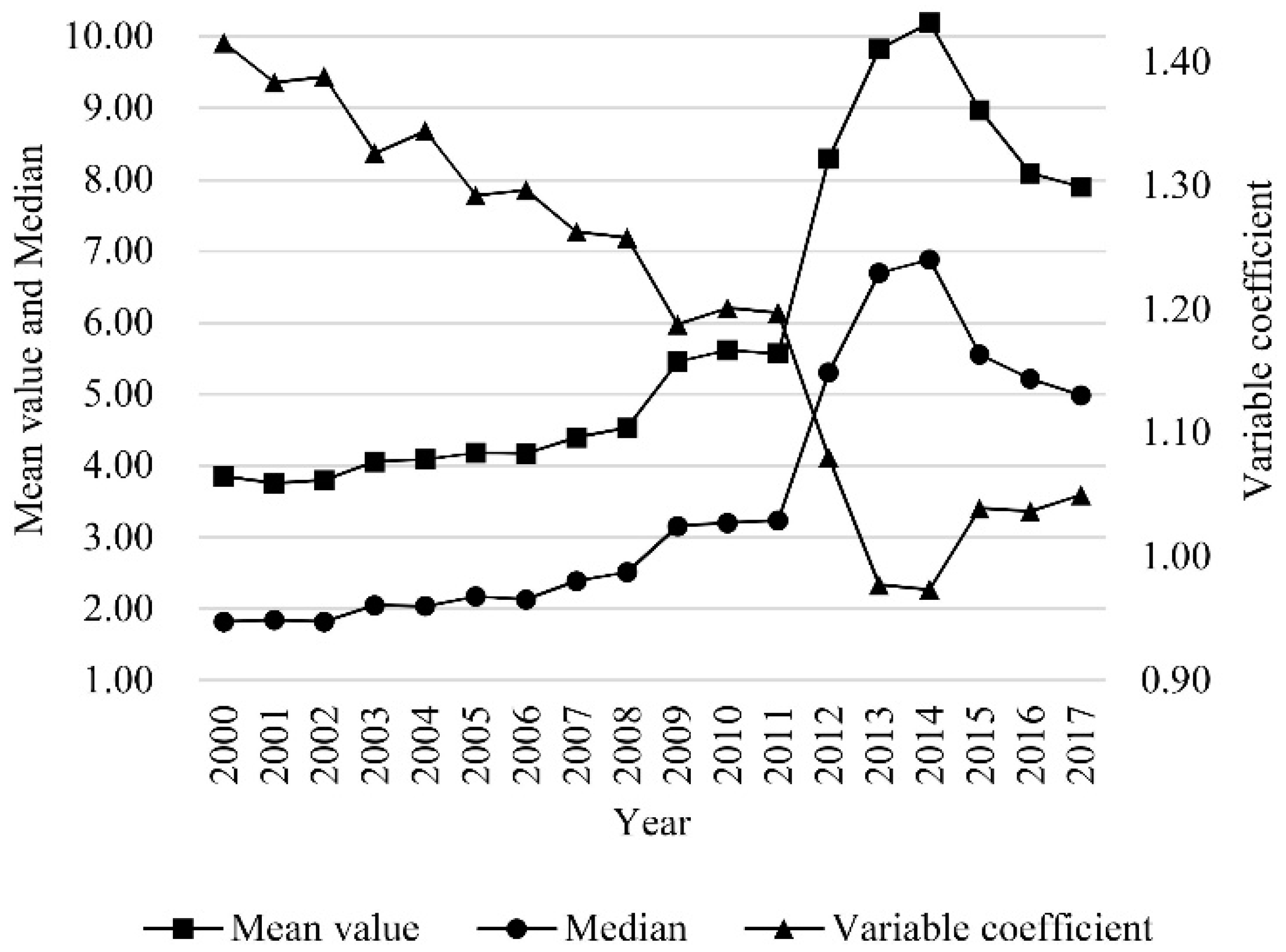
Figure 3 shows that from the evolution characteristics of the mean and median2 of the ESIs between all cities, there are roughly three time periods, as follows:
- From 2000 to 2011, the similarities among Chinese cities’ exports in the global market is relatively low. The mean values are always below six and the median also fluctuates at a low level. Especially between 2000 and 2008, these two indicators are in the low ranges of three to five and one to three, respectively.
- From 2011 to 2014, the similarity of exports between cities in the global market increases significantly. Compared with 2011, the mean and median in 2014 increased by 82.94% and 112.65%, respectively, indicating that during this period, the competition between different cities increased significantly and the complementarity weakened.
- From 2014 to 2017, the similarity of exports between cities in the global market declined. In 2017, the mean and median ESIs were 7.90 and 5.22, respectively, which are 22.47% and 24.24% lower than the 2014 peak.
ESI showed significant growth from 2011 to 2014 because some cities showed significant growth in export volume during this period. For example, in 2011–2012, the export trade of Changzhi, Bijie, and other cities showed significant growth, and the increase in the number of export commodities caused competition between these cities and other cities to become fiercer. In 2012, the exports of Changzhi increased by 1722.33% compared with that of 20113, while the exports of Bijie in 2012 increased by 1651.48% compared with 20114. Similarly, the decline between 2014 and 2017 was due to a significant decline in exports in some cities. For example, the export volume of Jinchang and Yinchuan decreased by 79%5 and 29.42%6, respectively, from 2014 to 2015. The sharp drop in exports means that the variety and quantity of goods will shrink, and competition with other cities will ease. The changes in ESI reflect that China’s urban export trade has experienced a period of adjustment. When some cities expand exports and participate in market competition, they fail to produce sustained economic benefits, so they reduce export scale, withdraw from competition, and choose a more suitable development model for themselves.
However, the coefficient of variation remains above one in most years, except 2013 and 2014, which also reflects the huge difference in the ESIs between cities. China’s hundreds of cities vary widely from one another in resource endowments and geographical advantages as well as in export structures. There are “city pairs” with similar export structures and fierce competition, and there are “city pairs” with different export structures and gentle competition.
3.1.2. Regional Analysis
Evolution of the ESI Network Structure among the Provincial Capitals
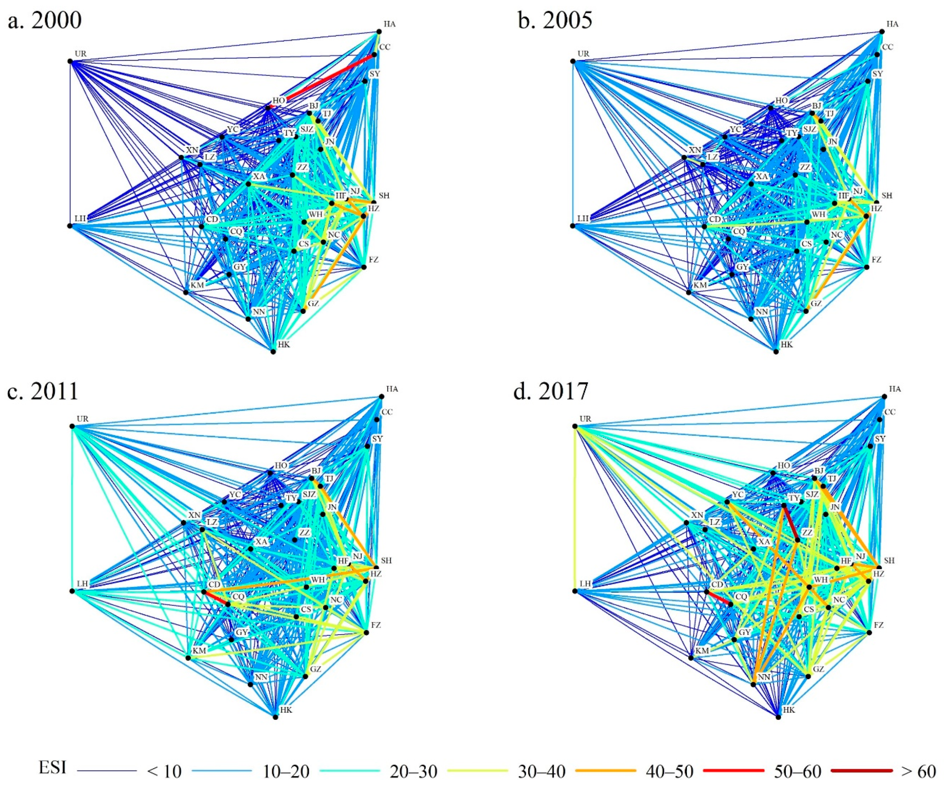
Figure 4 shows the ESI network between the provincial capitals in 2000, 2005, 2011, and 2017. The edge connecting the nodes is the ESI between two cities. Over time, the ESIs between the provincial capitals generally rose. Specifically, the average ESIs among the provincial capitals in 2000 was 14.54, and in 2005, 2011, and 2017, the values were 13.44, 15.49, and 16.65, respectively. This change shows that the level of competition among the export products of the provincial capitals in the global market increased and their complementarity weakened during this period.
From a spatial perspective, we see high ESIs between provincial capitals in the southeast coastal area from an early date, gradually spreading to the central and western regions. For example, the ESI of Chengdu (Western China) and Shanghai (Eastern China) was 21.17 in 2000 and increased to 33.36 in 2017. Figure 4 shows that the bright yellow high-value areas were still concentrated in the eastern region in 2000. However, by 2017, the high-value connections had expanded to the mid-west.
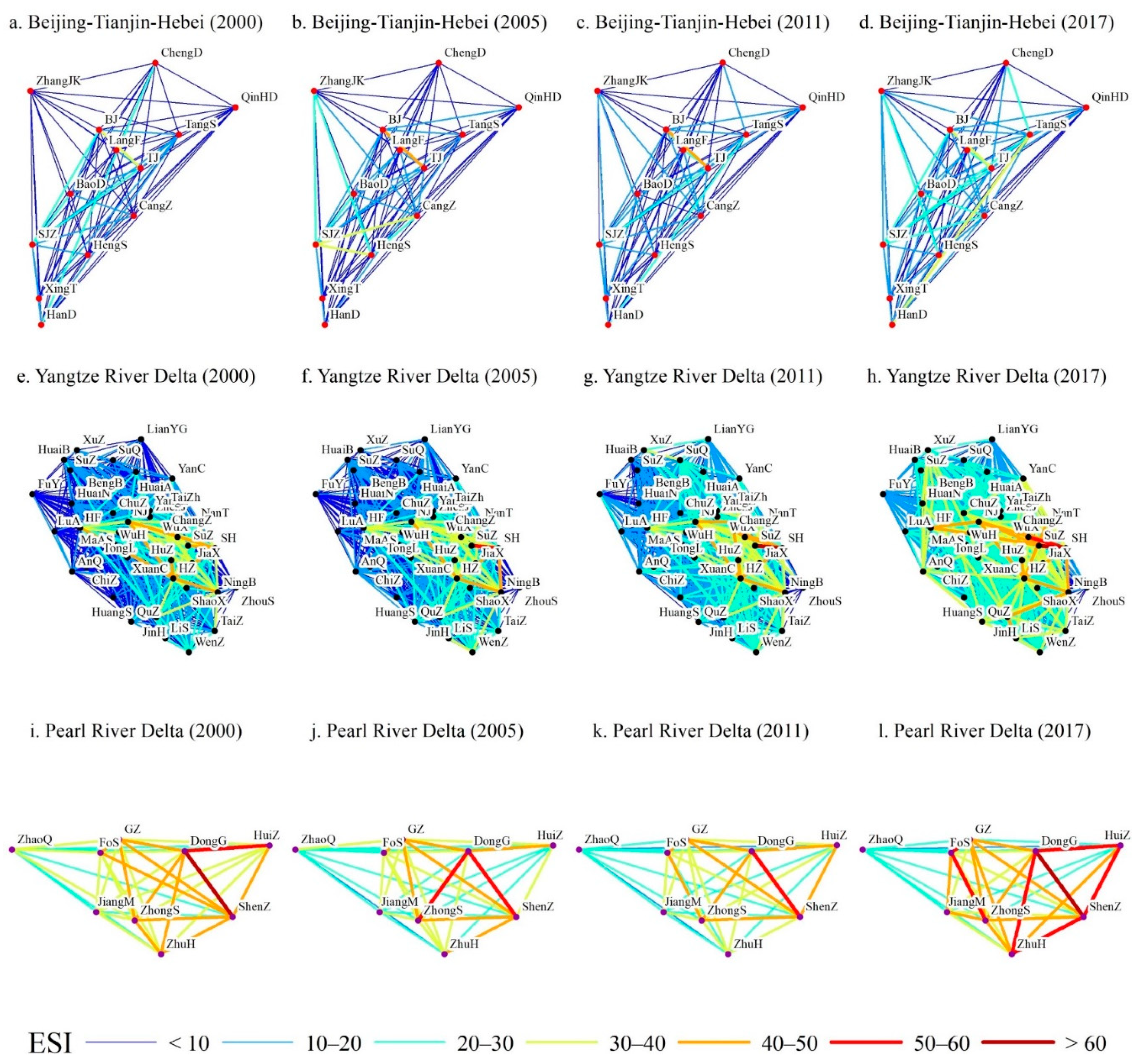
The ESI Network Structure Evolution among the BTH, YRD, and PRD
The urban agglomerations have certain differences. We found that the changes between cities in the PRD was not obvious from 2000 to 2017. In 2017, the average ESI among nine cities in the PRD was 36.90, a decrease of 1.91% when compared with 2000. Conversely, the average ESI among cities in the YRD increased by 78.17% between 2000 and 2017; the average ESI among cities in the BTH increased by 49.94% between 2000 and 2017. Therefore, the export competitive relationship of cities in the YRD and BTH significantly increased when compared with the PRD.
Moreover, a comparison of the three urban agglomerations shows that the cities in the PRD had the most prominent competitive relationship in the global market. Taking Dongguan and Shenzhen as examples, their ESI in 2000 was 63.14, while the average ESI of all cities in that year was only 3.86 (see Figure 3). In contrast, the competition between cities in the BTH is not obvious. Most city-pairs in the BTH have ESIs below 20 (see Figure 5). Because of the large number of city-pairs in YRD, there are many high (orange and red lines) and many low (blue lines) ESI values (see Figure 5).
3.2. The Relationship between AESI and GDP
Although previous studies on export competition between countries found that the competition relationship would strengthen with the growth of economic aggregate [10,11], they did not confirm whether there is a relationship between urban economic aggregate (represented by GDP) and the export competition pressure cities face.
3.2.1. Correlation between AESI and GDP
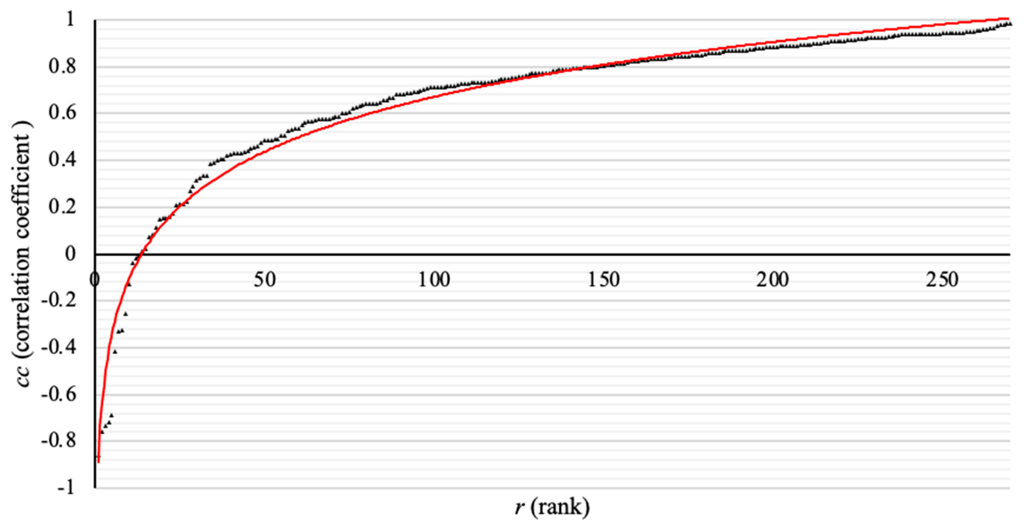
We analyzed the correlation between the GDP and AESI of each city from 2000 to 2017 to obtain the correlation coefficient (cc) of each city. We arranged the ccs in ascending order to form a scatter plot and draw a bit-order fitting curve (see Figure 6). For most cities, the correlation between the GDP and AESI is strong (cc accounts for a high proportion of over 0.5). Interestingly, more economically developed cities have a higher cc. For example, there are 11 cities with ccs above 0.95; among which, seven are developed cities in China’s east coast areas.
3.2.2. Causal Analysis of AESI and GDP
The existence of a correlation between these two indicators only points to the fact that the average competitive pressure that a city faces from other cities is related to its GDP. However, whether there is a causal relationship between the two variables needs further analysis. The panel Granger causality test provides a good method to address this issue.
All Cities
The panel unit root test results show that the AESI and GDP passed the unit root test after the first difference. However, they did not pass the panel cointegration test. Therefore, a second difference was performed. Subsequently, they passed the cointegration test after passing the unit root test. Therefore, the panel Granger causality test could be performed. Table 1 shows that the GDP and AESI demonstrate a two-way causal relationship for all cities.
Regional Analysis
The provincial capital GDP and AESI passed the panel unit root test after the first difference. Next, they passed the panel cointegration test (p < 0.1). Subsequently, in the panel Granger causality test, when the criterion is BIC, the Z-bar and Z-bar tilde did not reject HB (see Table 1). Therefore, at the provincial capital level, the Granger causality test results of the panel provide some support for the hypothesis that GDP is the Granger cause of the AESI. In BTH, the panel Granger causality test results show that HA is not strongly rejected (under the three criteria, only the p-value of the Z-bar met the requirements) and HB is not rejected at all (under the three criteria, the Z-bar and Z-bar tilde are not significant). So, relatively speaking, the causal analysis results for BTH were also more in favor of the hypothesis that GDP is the Granger cause of the AESI. The Granger causality test results show that, in the YRD, there was a two-way causality between city GDP and AESI. Table 1 shows that the null hypothesis is strongly rejected under both criteria. In PRD, the empirical results do not reject either HA or HB. Therefore, for the PRD cities, there is no proven causal relationship between the economic aggregate and the competitive pressure that each city faced from other cities. One possible reason is that the growth of PRD export volume and the degree of convergence of commodity structure are more influenced by foreign investment (as global capital radiates to PRD through Hong Kong), rather than mainly due to the spillover effect brought by the growth of economic aggregate. In 2017, the export volume of foreign-invested enterprises in PRD accounted for 46.85% of the total export volume of PRD, while the value of BTH was only 33.87%. The values for YRD and National were also lower than that for PRD, accounting for 45.82% and 43.19%, respectively. On the other hand, the foreign investment entering PRD, mainly in the manufacturing industry, can indeed generate relatively large export volumes. In 2017, the ratio of PRD’s foreign-invested enterprises’ exports to the amount of foreign capital utilized was 12.68, whereas the ratios in BTH and YRD were only 1.03 and 5.28. Simultaneously, AESI has no impact on GDP in PRD, because the competitive relationship between exports of cities in PRD is not generated by the gradual expansion of local enterprises, but directly caused by foreign capital, with obvious homogeneity at the beginning. Therefore, this competitive relationship has no strong economic impetus. This phenomenon shows that the export development modes of PRD, BTH, and YRD are different.
3.2.3. Relationship between ESI and Distance
Prior to the gravity model analysis, the following question needed to be confirmed: Is the ESI somehow related to distance?
All Cities
Regional Analysis
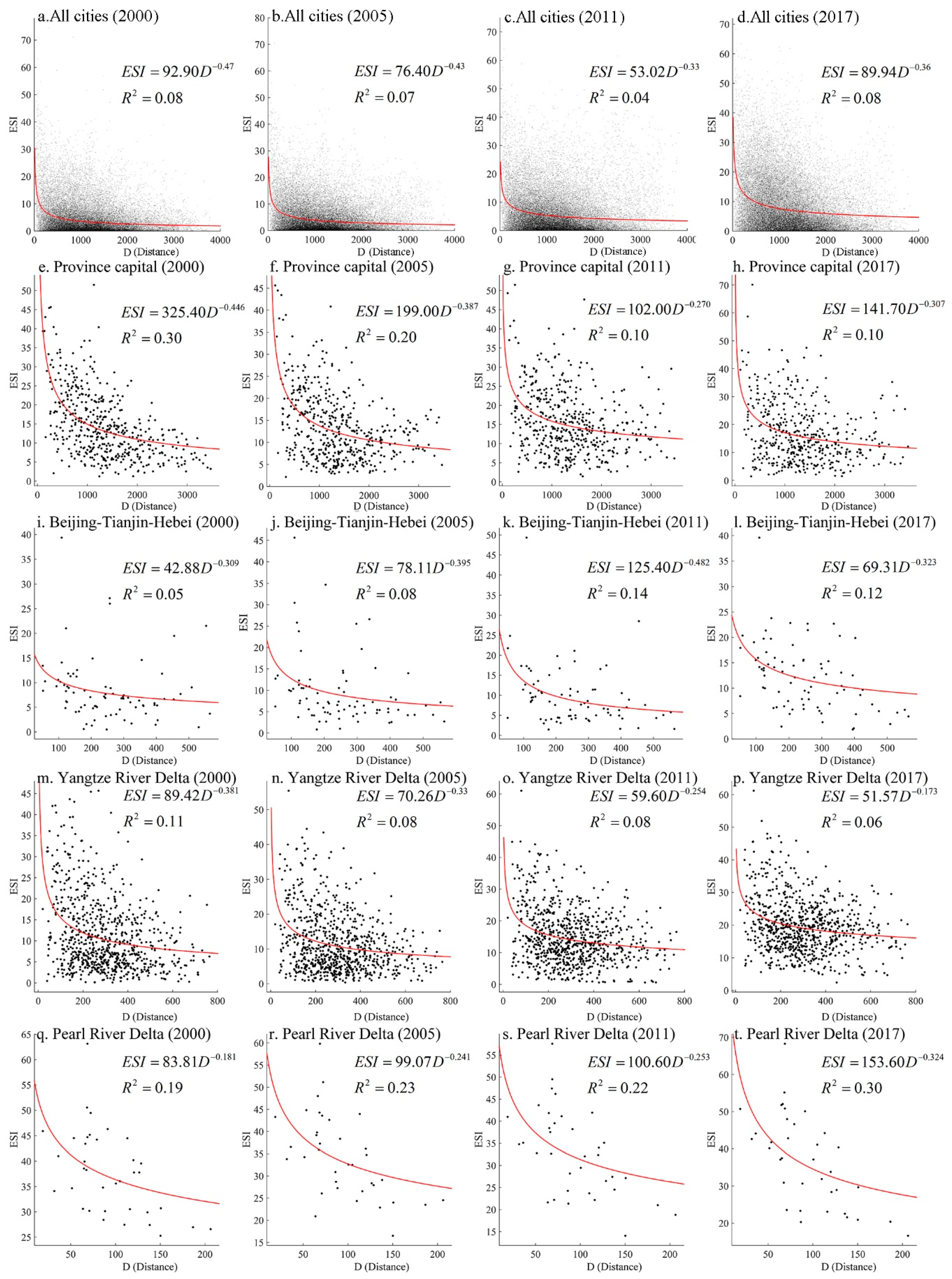
The fitting relationship between the ESI and the distance between provincial capitals and within urban agglomerations also roughly meets the power law decreasing trend. From the time evolution of the power index, the trend of the ESI decreasing with the increasing distance within the PRD intensified. In 2000, the absolute power exponent of the fitted curve of the ESI and the distance between the cities within the PRD was 0.181 (see Figure 7q). However, by 2017, the absolute value of the exponent increased to 0.324 (see Figure 7t). Therefore, the closer the cities were within the PRD, the higher the ESI, and the more competitive they were in the global market. Simultaneously, this trend of higher competition between closer cities became more pronounced over time. Conversely, in both the provincial capitals and YRD cities, the power index decreased from a relatively high value in 2000 to a relatively low value in 2017. The provincial capitals decreased from 0.446 to 0.307 (see Figure 7e,h) and the YRD decreased from 0.381 to 0.173 (see Figure 7m,p). For the provincial capitals and the YRD cities, the distance restriction effect of the export competition between cities weakened.
However, no matter how the exponent changes, there is no doubt that closer distance leads to higher ESI as a general trend. The finding, from the perspective of export competition, reaffirms the first law of geography: everything is related to everything else, but near things are more related than distant things [43].
3.2.4. Gravity Model: Relation between the ESI, GDP, and Distance
As we show, the ESI between cities is closely related to GDP and the geographical distance between cities:
- The GDP is the Granger cause of the export competitive pressure that cities face.
- The greater the distance between two cities, the less the competition between them.
For a deeper analysis of the comprehensive impact of GDP and distance on ESI, we propose the following model based on the gravity model: ESIijk = [θ·(GDPi GDPj)φ]/dijσ. ESIijk is the ESI of cities i and j in the global market (market k), representing the competition between them. GDPi and GDPj represent the economic aggregates of cities i and j, respectively. θ, φ, and σ are parameters. We should note that because the ESI has no directionality (ESIijk = ESIjik), we modeled the product of GDPi and GDPj as a whole. In general, the empirical analysis of a gravity model should first be converted into a linear logarithmic expression. Because ESIijk = 0, the logarithm cannot be formed. Therefore, a nonlinear least squares estimation (NLS) was performed and the 0 value was incorporated into the analysis.
At the level of all cities, the NLS estimates for all data show that, regardless of θ, φ, and σ, they are all p < 0.01. At the regional level, φ and σ differ significantly among the provincial capitals, BTH cities, and the cities of the PRD. For the PRD particularly, the values of φ and σ vary greatly (see Table 2, Column 6). This result reflects that GDP plays a much smaller role than the distance between cities in influencing the competition relationship between cities in PRD. As the above causality test has confirmed, in PRD, there is no significant causal relationship between the economic aggregate of a city and the competitive pressure faced by the city. However, YRD is different, as φ (0.1911) is slightly less than σ (0.2122). Compared with BTH and PRD, competition between cities in YRD is thus more closely affected by GDP and distance.
It is necessary to further explain the effect of GDP on the competitive pressures faced by urban exports. Economic growth in a city means that enterprises in the city accumulate more wealth and tend to invest in high-tech and high-value-added industries to gain higher profits [44,45], especially in the production of export commodities, such as high-tech products. In fact, the expansion of economic scale can indeed promote the export of high-tech products [46]. At the same time, economic growth will also expand the variety of export products [47]. As most cities expand their export products with economic growth, the proportion of overlap between them increases and competition between them becomes increasingly fierce.
At the international level, something similar is playing out. In the early stage, developed countries transfer part of their low-end production links and technologies to neigh-boring less developed countries. At this time, because the backward countries and developed countries are in different links of the value chain, they are more complementary to each other in the world trade market. But as the economies of poor countries grow, they have a stronger incentive to upgrade their industrial structures for higher profits. Thus began the challenge of the poor to the developed in the global market. Recent trade frictions between China and the US are a case in point [48].
4. Conclusions
In this study, the Export Similarity Index is used to measure the competitive relationship of Chinese cities in the global market, expanding the discussion of cities in the study of export trade competition. Based on the econometric model, the mechanism of competition is discussed. The main conclusions are as follows:
- From a national perspective, the intensity of the competition among cities in the global market first increased and then decreased from 2000 to 2017. Competition relationship change reflects the evolution and development of Chinese cities regarding industry and economic structure. Cities in different regions have different competition relationships in export trade, indicating that the export structure and basic characteristics of cities are related to their geographical location. Provincial capitals, as regional economic centers, have high levels of industrialization and urbanization and their industrial layout and export structure are relatively close. PRD, as the pioneer area of China’s reform and opening up, had its economy grow dramatically, accompanied by the introduction of foreign capital and the development of local industrialization [49,50]. Therefore, local foreign trade processing products in the PRD tend to be similar in category and the competition between them in the global market is more significant than for BTH and YRD.
- The GDP of each city was highly correlated with the AESI. Overall, the economic growth of cities and the pressure of export competition from other cities was related via cause and effect. However, at the regional level, the empirical results were more likely to support the GDP as the Granger cause of the AESI; that is, a city’s economic growth will intensify the export competition pressure that it faces. Confirmation of such a causal relationship lays a foundation for the use of the gravity model in this study.
- The evolution of the urban export structure in China is related to geographical proximity, to some extent. The ESI shows a trend of decreasing with increasing geographical distance. The proximity of a geographical location means there are similar development conditions [51], a higher possibility of economic factor spillover, a higher probability of export product convergence, and a more evident competitive relationship in the market.
- The relationships among the ESI, the GDP, and geographical distance can be incorporated well into the gravity model. If the economic aggregate of the two cities is larger and the geographical distance is smaller, then the export similarity of the two cities will be higher, and the competition in the global market will be more obvious. However, the impact of GDP and distance on ESI varies in different regions. For example, in BTH, the influence of distance on the competition between cities is more obvious than that of YRD and PRD. The success of empirical research using the gravity model reflects two basic characteristics of Chinese cities in developing export trading. First, economic growth provides the capital, technology, and human resources for increasing the variety of export products and upgrading the export structure. However, the path and direction of the export trade development tend to converge, resulting in an increased ESI and progressively fierce competition for global markets. Second, the ESI has obvious geographical proximity characteristics. This rule makes a high ESI more likely to occur in cities that are geographically adjacent, and competition in the global market is more obvious.
With the increasing integration of urban agglomerations in China, the export competition caused by economic growth and geographical proximity intensifies, which requires reasonable regulation by the government and enterprises. Different cities should have different functions in the region [52,53] and export different products. If there is too much production and export of the same or similar products, adjacent regions become prone to excessive competition and internal friction, resulting in diseconomies of scale. China’s urbanization process and economic development stage are different from those in the early stage of reform and opening up, which requires more detailed and efficient regional coordination and management.
There is competition between cities for exports not only in China, but also in countries around the world. The cities of Incheon and Busan in South Korea, for example, compete with each other for exports [54]. On the other hand, the closer the distance between regions is, the more likely technology spillovers will occur, bringing about industrial structure convergence and higher export similarity. In the United States, the eastern states of Ohio and Indiana are close to each other, and their leading export products are transportation equipment (Wikipedia). There has long been competition between these regions. Therefore, the results of this paper are enlightening for not only the development of export trade in Chinese cities but also the development of export trade in cities/states in other large trading countries.
There are still some deficiencies in this paper. First, the factors that affect the competition of export trade between cities include not only GDP and distance, but also innovation cooperation between cities and the policies of central and local governments for the external economic development of cities. We will include further, more comprehensive factors in the future. Second, the data need to be updated further, as in recent years, Sino–US trade frictions and the COVID-19 pandemic have greatly affected the exports of Chinese cities. We will collect and sort updated data to improve our research. In addition, there is a lot of room to expand the scope of the research on competition in urban export trade. In the future, we will discuss in depth the influence of urban export trade competition on urban development and whether and how it affects the structure of urban export commodities.
Author Contributions
Conceptualization, E.L.; methodology, E.L.; software, E.L.; validation, Y.C.; formal analysis, M.L.; investigation, G.H.; resources, Y.C.; data curation, M.L.; writing—original draft preparation, E.L.; writing—review and editing, E.L.; visualization, E.L.; supervision, Y.C.; project administration, Y.C.; funding acquisition, Y.C. All authors have read and agreed to the published version of the manuscript.
Funding
This research was funded by the National Natural Science Foundation of China (grant number 42171173, 42001125,42171171), Work Start-up Funding Program for High-Level Talents of Jinling Institute of Technology (grant numbers jit-b-202202), and the Humanities and Social Science Research Project of the Ministry of Education of China (grant number 19YJAZH023, 20YJC790093).
Institutional Review Board Statement
Not applicable.
Informed Consent Statement
Not applicable.
Data Availability Statement
The data used to support the findings of this study are available from the corresponding author upon request.
Acknowledgments
Thanks to Yuqi Lu and Qi Cui for giving some suggestions on this study.
Conflicts of Interest
The authors declare no conflict of interest.
| 1 | The BTH urban agglomerations include the cities of Beijing and Tianjin as well as Hebei Province, with a total of 13 cities. According to the “Outline of the Regional Integration Development Plan of the Yangtze River Delta” (http://www.gov.cn/zhengce/2019-12/01/content_5457442.htm (accessed on 14 March 2021)), the YRD urban agglomerations include Jiangsu Province, Zhejiang Province, Anhui Province, and the city of Shanghai. Because of a data defect, Bozhou City in Anhui Province is not included in the analysis. With reference to the latest plan for the Guangdong–Hong Kong–Macao Greater Bay Area (http://www.gov.cn/zhengce/2019-02/18/content_5366593.htm#1 (accessed on 15 March 2021)) released in recent years, this study takes the cities of Guangzhou, Shenzhen, Zhuhai, Foshan, Huizhou, Dongguan, Zhongshan, Jiangmen, and Zhaoqing as the PRD urban agglomerations. |
| 2 | Because there are 270 cities in total, the ESI has 269 + 268 + … + 1 = 36,315 values. The mean is the average of 36,315 ESIs; the median is the median value of 36,315 ESIs. |
| 3 | Data source: Statistical Yearbook of Changzhi City. |
| 4 | Data source: China Regional Economic Statistics Yearbook. |
| 5 | Data source: Statistical Bulletin of Jinchang National Economic and Social Development. |
| 6 | Data source: Yinchuan Yearbook. |
References
- Zhang, C.; Xingchen, J.I.; Finance, S.O. The evolution and logic of forward-looking monetary policy. Chin. Rew. Financ. Stud. 2017, 9, 33–42. [Google Scholar]
- He, Y.; Bai, X. The Trade competitiveness and similarities of the urban agglomerations in the middle reaches of the Yangtze River. Contemp. Econ. Manag. 2017, 39, 51–56. [Google Scholar]
- Bao, J.; Gao, S.; Ge, J. Dynamic land use and its policy in response to environmental and social-economic changes in China: A case study of the Jiangsu coast (1750–2015). Land Use Policy 2019, 82, 169–180. [Google Scholar] [CrossRef]
- Chen, F.; Yu, M.; Zhu, F.; Shen, C.; Zhang, S.; Yang, Y. Rethinking rural transformation caused by comprehensive land consolidation: Insight from program of whole village restructuring in Jiangsu province, China. Sustainability 2018, 10, 2029. [Google Scholar] [CrossRef] [Green Version]
- Crespo, N.; Simoes, N.; Moreira, S. Bringing geography into the analysis of trade competition. Appl. Econ. Lett. 2019, 26, 948–953. [Google Scholar] [CrossRef]
- Molendowski, E.; Polan, W. Poland in the single European market-changes in the similarity of import and export structures in comparison with the EU-10 countries in 2004–2017. Int. J. Manag. Econ. 2020, 56, 20–30. [Google Scholar]
- Kreinin, M.E.; Plummer, M.G. Regional groupings, discrimination, and erosion of preferences: Effects of EU enlargement on the Mediterranean Basin. J. Int. Trade Econ. Dev. 2007, 16, 213–230. [Google Scholar] [CrossRef]
- Sun, Z.; Li, X. A study on the comparative advantage and growth potential of agricultural trade between China and EU. Res. Agric. Mod. 2015, 36, 521–527. [Google Scholar]
- Wang, P.-Z.; Liu, X.-J. Comparative analysis of Export Similarity Index between China and EU. In Proceedings of the 2015 International Conference on Management Science and Management Innovation, Guilin, China, 15–16 August 2015; Advances in Economics, Business and Management Research 62015; Wang, M., Ed.; Atlantis Press: Dordrecht, The Netherlands, 2015; pp. 222–227. [Google Scholar]
- Dean, J.M.; Fung, K.C. Measuring vertical specialization: The case of China. Rev. Int. Econ. 2011, 19, 609–625. [Google Scholar] [CrossRef]
- Schott, P.K. The relative sophistication of Chinese exports. Econ. Policy 2008, 23, 5–49. [Google Scholar] [CrossRef]
- Wang, Z.; Wei, S.J. What Accounts for the Rising Sophistication of China’s Exports? University of Chicago Press: Chicago, IL, USA, 2010. [Google Scholar]
- Moreira, M.M. Fear of China: Is there a future for manufacturing in Latin America? World Dev. 2007, 35, 355–376. [Google Scholar] [CrossRef] [Green Version]
- Caselli, F.G. China’s rise, asymmetric trade shocks and exchange rate regimes. Rev. Int. Econ. 2019, 27, 1–35. [Google Scholar] [CrossRef] [Green Version]
- Xu, B. The sophistication of exports: Is China special? China Econ. Rev. 2010, 21, 482–493. [Google Scholar] [CrossRef]
- Athukorala, P.-C. Post-crisis export performance: The Indonesian experience in regional perspective. Bull. Indones. Econ. Stud. 2006, 42, 177–211. [Google Scholar] [CrossRef]
- Finger, J.M.; Kreinin, M.E. A measure of export similarity’ and its possible uses. Econ. J. 1979, 89, 905–912. [Google Scholar] [CrossRef]
- Liu, C.L.; Xu, J.Q.; Zhang, H. Competitiveness or complementarity? A dynamic network analysis of international agri-trade along the belt and road. Appl. Spat. Anal. Policy 2020, 13, 349–374. [Google Scholar] [CrossRef]
- Nguyen, T.N.A.; Pham, T.H.H.; Vallee, T. Similarity in trade structure: Evidence from ASEAN+3. J. Int. Trade Econ. Dev. 2017, 26, 1000–1024. [Google Scholar] [CrossRef]
- Lu, S.; Dickerson, K. The United States-Korea free trade agreement (KORUS) and its impacts on China’s textile and apparel exports to the United States. Cloth Text Res. J. 2012, 30, 300–314. [Google Scholar] [CrossRef] [Green Version]
- Rondinella, S.; Agostino, M.; Demaria, F.; Drogue, S. Similarity and competition in the agri-food trade among European Mediterranean countries. Int. Trade J. 2019, 33, 444–468. [Google Scholar] [CrossRef]
- Adewuyi, A.O.; Awodumi, O.B. Biomass energy consumption, economic growth and carbon emissions: Fresh evidence from West Africa using a simultaneous equation model. Energy 2017, 119, 453–471. [Google Scholar] [CrossRef]
- Chaiboonsri, C.; Sriboonjit, J.; Sriwichailamphan, T.; Chaitip, P.; Sriboonchitta, S. A panel cointegration analysis: An application to international tourism demand of Thailand. Ann. Univ. Petrosani Econ. 2010, 10, 69–86. [Google Scholar]
- Srivastava, S.; Talwar, S. Decrypting the dependency relationship between the triad of foreign direct investment, economic growth and human development. J. Dev. Areas 2020, 54, 1–14. [Google Scholar] [CrossRef]
- Wongsrida, S.; Chaitip, P. Effect of macro factor volatility on the returns of financial sector in Southeast Asian stock markets. Chin. Bus. Rev. 2014, 13, 28–33. [Google Scholar]
- Levin, A.; Lin, C.-F.; Chu, C.-S.J. Unit root tests in panel data: Asymptotic and finite-sample properties. J. Econom. 2002, 108, 1–24. [Google Scholar] [CrossRef]
- Kao, C. Spurious regression and residual-based tests for cointegration in panel data when the cross-section and time-series dimensions are comparable. Economet. J. 1997, 90, 1–44. [Google Scholar] [CrossRef]
- Pedroni, P. Critical values for cointegration tests in heterogeneous panels with multiple regressors. Oxf. Bull. Econ. Stats. 1999, 61, 653–670. [Google Scholar] [CrossRef]
- Westerlund, J. Testing for error correction in panel data. Oxf. Bull. Econ. Stats. 2010, 69, 709–748. [Google Scholar] [CrossRef] [Green Version]
- Wang, F.; Liu, Y. Panel Granger Test on urban land expansion and fiscal revenue growth in China’s prefecture-level cities. Acta Geogr. Sinica 2013, 68, 1595–1606. [Google Scholar]
- Lu, Y.-D.; Li, D. Trade structure, division economy and the welfare effect of regional service trade liberalization. Int. Econ. Trade Res. 2012, 5, 15–34. [Google Scholar]
- Granger, C.W. Investigating causal relations by econometric models and cross-spectral methods. Econometrica 1969, 37, 424–438. [Google Scholar] [CrossRef]
- Dumitrescu, E.-I.; Hurlin, C. Testing for Granger non-causality in heterogeneous panels. Econ. Model. 2012, 29, 1450–1460. [Google Scholar] [CrossRef] [Green Version]
- Akaike, H. A new look at the statistical model identification. IEEE Trans. Automat. Contr. 1974, 19, 716–723. [Google Scholar] [CrossRef]
- Schwarz, G. The Bayesian information criterion. Ann. Statist. 1978, 6, 461–464. [Google Scholar]
- Hannan, E.J.; Quinn, B.G. The determination of the order of an autoregression. J. R. Stat. Soc. B. 1979, 41, 190–195. [Google Scholar] [CrossRef]
- Melitz, J.; Toubal, F. Somatic distance, trust and trade. Rev. Int. Econ. 2019, 27, 786–802. [Google Scholar] [CrossRef] [Green Version]
- Liu, L.W.; Zhang, M. High-speed rail impacts on travel times, accessibility, and economic productivity: A benchmarking analysis in city-cluster regions of China. J. Transp. Geogr. 2018, 73, 25–40. [Google Scholar] [CrossRef]
- Fratianni, M.; Marchionne, F. Trade costs and economic development. Econ. Geogr. 2012, 88, 137–163. [Google Scholar] [CrossRef]
- Shaopai, L.; Jipeng, T.; Lin, L. A case study of Shanghai Disneyland on spatial structure forecast for proposed scenic spot market: Modification and its application of gravity model. Acta Geogr. Sinica 2016, 71, 304–321. [Google Scholar]
- Tang, F.; Zhou, X.; Wang, L.; Zhang, Y.; Fu, M.; Zhang, P. Linking ecosystem service and MSPA to construct landscape ecological network of the Huaiyang Section of the Grand Canal. Land 2021, 10, 919. [Google Scholar] [CrossRef]
- Surya, B.; Ahmad, D.N.A.; Sakti, H.H.; Sahban, H. Land use change, spatial interaction, and sustainable development in the metropolitan urban areas, South Sulawesi Province, Indonesia. Land 2020, 9, 95. [Google Scholar] [CrossRef] [Green Version]
- Tobler, W.R. A computer movie simulating urban growth in the Detroit region. Econ. Geogr. 1970, 46, 234–240. [Google Scholar] [CrossRef]
- Rastvortseva, S.N. Innovative path of the regional economy’s departure from the previous path-dependent development trajectory. Ekon. Reg. 2020, 16, 28–42. [Google Scholar] [CrossRef]
- Ravselj, D.; Aristovnik, A. The impact of private research and development expenditures and tax incentives on sustainable corporate growth in selected OECD countries. Sustainability 2018, 10, 2304. [Google Scholar] [CrossRef] [Green Version]
- Mehrara, M.; Seijani, S.; Karsalari, A.R. Determinants of high-tech export in developing countries based on Bayesian model averaging. Zb. Rad. Ekon. Fak. Rije. 2017, 35, 199–215. [Google Scholar]
- Pham, C.S.; Ulubasoglu, M.A. The role of endowments, technology and size in international trade: New evidence from product-level data. J. Int. Trade Econ. Dev. 2016, 25, 913–937. [Google Scholar] [CrossRef]
- Boylan, B.M.; McBeath, J.; Wang, B. US–China relations: Nationalism, the trade war, and COVID-19. Fudan. J. Hum. Soc. Sci. 2021, 14, 23–40. [Google Scholar] [CrossRef]
- Zhou, C.; Wang, Y.; Xu, Q.; Li, S. The new process of urbanization in the Pearl River Delta. Geogr. Res. 2019, 38, 45–63. [Google Scholar]
- Xun, L.I.; Xin Zheng, D. Spatial aggregation and location selection of FDI base on empirical analysis Zhujiangl river delta of China. Sci. Geogra. Sinica 2007, 27, 636–641. [Google Scholar]
- Sheng, G. Multiple correlation effect of regional economic growth and its empirical test. Economist 2018, 4, 34–41. [Google Scholar]
- Wang, S.; Gao, S.; Wang, Y. Spatial structure of the urban agglomeration based on space of flows: The study of the Pearl river Delta. Geogr. Res. 2019, 38, 1849–1861. [Google Scholar]
- Wang, C.; Cao, Y.; Chen, G. Study on urban network of Yangtze River Delta region based on producer services. Geogr. Res. 2014, 33, 323–335. [Google Scholar]
- Jung-Dong, P.; Kyong-Hui, K. Comparison of competitiveness by export item of Incheon and Busan in China. Korean-Chin. Soc. Sci. Stud. 2010, 8, 31–56. [Google Scholar]
Figure 1.
The research framework.

Figure 2.
The study area.

Figure 3.
The mean, median, and variable coefficient of the ESIs between each pair of cities from 2000 to 2017.
Figure 3.
The mean, median, and variable coefficient of the ESIs between each pair of cities from 2000 to 2017.

Figure 4.
The ESI network between provincial capitals in 2000, 2005, 2011, and 2017.

Figure 5.
The ESI network of the three urban agglomerations. (Each dot represents a city. The redder and wider the line between cities, the fiercer the export competition between the two cities.)
Figure 5.
The ESI network of the three urban agglomerations. (Each dot represents a city. The redder and wider the line between cities, the fiercer the export competition between the two cities.)

Figure 6.
The correlation coefficient of the AESI and GDP on the fitting curve in ascending order.

Figure 7.
The scatter diagrams and fitting curves of the ESI and distance between cities.


Table 1.
The results of panel Granger causality test for all cities, provincial capitals, and three urban agglomerations.
Table 1.
The results of panel Granger causality test for all cities, provincial capitals, and three urban agglomerations.
| Region | Criterion | Statistics | Optimal Lag Length | HA: GDP Is not the Granger Cause of AESI | Optimal Lag Length | HB: AESI Is Not the Granger Cause of GDP |
|---|---|---|---|---|---|---|
| all cities | AIC | W-bar | 3 | 13.3684 | 3 | 6.5296 |
| Z-bar | 69.5531 *** | 23.6775 *** | ||||
| Z-bar Tilde | 21.1994 *** | 4.8518 *** | ||||
| BIC | W-bar | 3 | 13.3684 | 1 | 1.56622 | |
| Z-bar | 69.5531 *** | 6.5323 *** | ||||
| Z-bar Tilde | 21.1994 *** | 2.9908 *** | ||||
| HQIC | W-bar | 3 | 13.3684 | 3 | 6.5296 | |
| Z-bar | 69.5531 *** | 23.6775 *** | ||||
| Z-bar Tilde | 21.1994 *** | 4.8518 *** | ||||
| provincial capitals | AIC | W-bar | 3 | 10.0982 | 3 | 6.4667 |
| Z-bar | 16.1344 *** | 7.8799 *** | ||||
| Z-bar Tilde | 5.8643 *** | 2.2536 ** | ||||
| BIC | W-bar | 3 | 10.0982 | 1 | 1.3879 | |
| Z-bar | 16.1344 *** | 1.5272 | ||||
| Z-bar Tilde | 5.8643 *** | 0.5946 | ||||
| HQIC | W-bar | 3 | 10.0982 | 3 | 6.4667 | |
| Z-bar | 16.1344 *** | 7.8799 *** | ||||
| Z-bar Tilde | 5.8643 *** | 2.2536 ** | ||||
| BTH | AIC | W-bar | 3 | 6.2438 | 3 | 3.3452 |
| Z-bar | 4.7747 *** | 0.5081 | ||||
| Z-bar Tilde | 0.9147 | −0.6057 | ||||
| BIC | W-bar | 3 | 6.2438 | 1 | 1.1876 | |
| Z-bar | 4.7747 *** | 0.4783 | ||||
| Z-bar Tilde | 0.9147 | −0.0225 | ||||
| HQIC | W-bar | 3 | 6.2438 | 3 | 3.3452 | |
| Z-bar | 4.7747 *** | 0.5081 | ||||
| Z-bar Tilde | 0.9147 | −0.6057 | ||||
| YRD | AIC | W-bar | 3 | 15.7630 | 3 | 7.7811 |
| Z-bar | 32.9539 *** | 12.3446 *** | ||||
| Z-bar Tilde | 13.0591 ** | 4.0444 *** | ||||
| BIC | W-bar | 3 | 15.7630 | 3 | 7.7811 | |
| Z-bar | 32.9539 *** | 12.3446 *** | ||||
| Z-bar Tilde | 13.0591 ** | 4.0444 *** | ||||
| HQIC | W-bar | 3 | 15.7630 | 3 | 7.7811 | |
| Z-bar | 32.9539 *** | 12.3446 *** | ||||
| Z-bar Tilde | 13.0591 ** | 4.0444 *** | ||||
| PRD | AIC | W-bar | 3 | 4.0850 | 2 | 2.3188 |
| Z-bar | 1.3288 | 0.4782 | ||||
| Z-bar Tilde | −0.1811 | −0.2197 | ||||
| BIC | W-bar | 1 | 1.2150 | 1 | 0.5300 | |
| Z-bar | 0.4560 | −0.9970 | ||||
| Z-bar Tilde | 0.0225 | −1.0100 | ||||
| HQIC | W-bar | 3 | 4.0850 | 2 | 2.3188 | |
| Z-bar | 1.3288 | 0.4782 | ||||
| Z-bar Tilde | −0.1811 | −0.2197 |
Note: ** p < 0.05; *** p < 0.01. W-bar = average Wald statistic; Z-bar = standardized average Wald statistic (
); Z-bar tilde = standardized average statistic ().
Table 2.
The gravity model results.
| Statistics | All Cities | Regional Level | |||
|---|---|---|---|---|---|
| ProvinceCapital | BTH | YRD | PRD | ||
| 0.0073 *** (0.0002) | 1.5555 *** (0.1905) | 0.1749 *** (0.0623) | 0.0904 *** (0.0071) | 29.226 *** (5.7968) | |
| 0.2630 *** (0.0007) | 0.1161 *** (0.0029) | 0.1718 *** (0.0088) | 0.1911 *** (0.0020) | 0.0343 *** (0.0051) | |
| 0.2556 *** (0.0014) | 0.2296 *** (0.0079) | 0.3298 *** (0.0264) | 0.2112 *** (0.0057) | 0.2224 *** (0.0170) | |
| 0.53 | 0.81 | 0.76 | 0.84 | 0.95 | |
Note: The standard error is in parentheses. *** p < 0.01.
Publisher’s Note: MDPI stays neutral with regard to jurisdictional claims in published maps and institutional affiliations. |
© 2022 by the authors. Licensee MDPI, Basel, Switzerland. This article is an open access article distributed under the terms and conditions of the Creative Commons Attribution (CC BY) license (https://creativecommons.org/licenses/by/4.0/).
Share and Cite
MDPI and ACS Style
Li, E.; Chen, Y.; Hu, G.; Lu, M. Competition between Export Cities in China: Evolution and Influencing Factors. Land 2022, 11, 201. https://0-doi-org.brum.beds.ac.uk/10.3390/land11020201
AMA Style
Li E, Chen Y, Hu G, Lu M. Competition between Export Cities in China: Evolution and Influencing Factors. Land. 2022; 11(2):201. https://0-doi-org.brum.beds.ac.uk/10.3390/land11020201
Chicago/Turabian StyleLi, Enkang, Yu Chen, Guojian Hu, and Mengqiu Lu. 2022. "Competition between Export Cities in China: Evolution and Influencing Factors" Land 11, no. 2: 201. https://0-doi-org.brum.beds.ac.uk/10.3390/land11020201
Note that from the first issue of 2016, this journal uses article numbers instead of page numbers. See further details here.