
Analyzing the Effects of Land Cover Change on the Water Balance for Case Study Watersheds in Different Forested Ecosystems in the USA


1
KBR, Inc., Contractor to the U.S. Geological Survey Earth Resources Observation and Science (EROS) Center, Sioux Falls, SD 57198, USA
2
U.S. Geological Survey Earth Resources Observation and Science (EROS) Center, Sioux Falls, SD 57198, USA
*
Author to whom correspondence should be addressed.
Land 2022, 11(2), 316; https://0-doi-org.brum.beds.ac.uk/10.3390/land11020316
Submission received: 24 January 2022
/
Revised: 16 February 2022
/
Accepted: 19 February 2022
/
Published: 21 February 2022
(This article belongs to the Special Issue Impacts of Land Use and Land Cover Change on Hydrological Systems)
Abstract
:We analyzed impacts of interannual disturbance on the water balance of watersheds in different forested ecosystem case studies across the United States from 1985 to 2016 using a remotely sensed long-term land cover monitoring record (U.S. Geological Survey Land Change Monitoring, Assessment, and Projection (LCMAP) Collection 1.0 Science products), gridded precipitation and evaporation data, and streamgaging data using paired watersheds (high and low disturbance). LCMAP products were used to quantify the timing and degree of interannual disturbance and to gain a better understanding of how land cover change affects the water balance of disturbed watersheds. In this paper, we present how LCMAP science products can be used to improve knowledge for hydrologic modeling, climate research, and forest management. Anthropogenic influences (e.g., dams and irrigation diversions) often minimize the impacts of land cover change on water balance dynamics when compared to interannual fluctuations of hydroclimatic events (e.g., drought and flooding). Our findings show that each watershed exhibits a complex suite of influences involving climate variables and other factors that affect each of their water balances differently when land cover change occurs. In this study, forests within arid to semi-arid climates experience greater water balance effects from land cover change than watersheds where water is less limited.
1. Introduction
Connections between land cover change and watershed hydrology have been examined at a variety of spatial and temporal scales [1,2,3]. However, the roles of climate and land use changes vary from watershed to watershed because when, where, and how processes occur all have different impacts on hydrology and are dependent on landscape position and timing of events such as precipitation and drought [1,4]. Land cover change is typically thought to be a local phenomenon where impacts from disturbance decrease with increasing spatial scale. In contrast, the influence of regional climate variables may be thought to affect watersheds of different sizes in the same region similarly. Impacts on streamflow and runoff in tropical and humid climates are fundamentally different because erosion can play a much larger role [5], whereas runoff is suggested to be affected equally by climate and land cover change in arid regions [6,7]. Previous studies have also investigated the relative importance of how precipitation and land use/land cover changes affect streamflow and found that both factors affect hydrology [8]. By examining disturbance and relatively stable periods, statistical relationships between land cover change and precipitation can be established to gain a better understanding of relative importance of the two influences [9]. Thus, generalization of various land cover and climate controls on watershed hydrology in different environments is attainable but requires sufficient data and knowledge of site-specific land cover change, precipitation patterns, geomorphology, and human activities. Debates regarding the impact of land change on streamflow reinforce the science communities’ need for new strategies coupled with detailed land cover change information at the watershed scale [4]. Positive and negative feedbacks vary with time, producing short-term responses potentially differing from long-term responses.
In this study, we aim to address the questions: (1) Does land cover change in forested ecosystems with different disturbance regimes play a leading role in changes to the water balance in the United States? and (2) What relative roles do land cover change and precipitation play in changing the water balance in forested ecosystems with different disturbance regimes?
Remote sensing is the most efficient and effective means for studies involving large-scale land cover change analyses. Recent advances in technologies and methodological innovation using algorithms designed to detect landscape changes from spaceborne observations have greatly advanced. As our understanding of land cover processes has improved, the means to observe them at various spatial and temporal scales has expanded investigations into a wide variety of hydrologic aspects of land cover change involving vegetation canopy and/or shrub cover change (e.g., [10,11,12]), wetland and crop monitoring (e.g., [13,14,15,16,17]), and hydrological assessments of surface runoff (e.g., [18,19]) and subsurface features such as soil moisture and groundwater (e.g., [20,21]).
Human and natural alterations to land surface processes change how precipitation is transported, evaporated, or infiltrated. One of the modifications that can substantially affect various components of global, regional, and local water cycles, including overland flow or runoff, is land cover or land change. Numerous publications note effects of land cover change involving flooding, low flows, and more generally, water yield [5,22,23,24,25,26,27,28,29,30,31], but these studies had limited scope, were regionally based, or did not involve large-scale, widely applicable land cover data. Previous studies have also conducted paired watershed case studies examining the water balance of forested ecosystems, but they primarily focused on runoff and fluvial transport [32,33], effects of forest thinning treatments [34], evapotranspiration response to forest regeneration [35], and connections to groundwater [36]. Here, we present a new analysis using a cutting-edge suite of data products to analyze connections between land cover change and a watershed’s water balance in ways previously unattainable. The U.S. Geological Survey (USGS) Land Change Monitoring, Assessment, and Projection (LCMAP) initiative has developed a new suite of annual land change products [37] that provide spatial and temporal information for the entire contiguous United States (CONUS) at 30-m resolution covering our study period from 1985 to 2016. To investigate how land cover data with annual temporal frequency could inform a variety of hydrologic studies, we examined annual land cover change along with precipitation, streamflow, and evaporation patterns to elucidate how land change affects the water balance in watersheds with both relatively stable (herein referred to as low-disturbance: LD) or changing (herein referred to as high-disturbance: HD) land cover based on LCMAP land cover change products.
We hypothesized that (1) changes in land cover derived from annual land cover products provide a new toolset to aid explanations of changes or differences in the magnitude of water balance components and (2) annual land cover and land cover change data can enhance the ability of forest managers in assessing water balance changes in the future for a range of watershed characteristics.
2. Materials and Methods
Analysis of land cover change was conducted using representative watershed pairs that exhibited varying levels of disturbance in the form of primary land cover class changes, which were calculated from LCMAP science products [37]. Within each watershed pair case study, we used LCMAP science products to identify an HD watershed that experienced a heightened frequency of land cover class change compared to its companion LD watershed that had relatively stable land cover classification throughout the study period. Three categories of land change conversions represent roughly 85% of national-level land cover class changes in the United States: 51% were tree cover to grass/shrub (or vice versa), 25% were cropland to grass/shrub (or vice versa), and 9% were conversions to developed land [38]. To address the category of greatest proportion of land change, we restricted our study sites to forested watershed pairs meeting the following criteria: (1) one LD watershed with minimal to no land cover change during the study period, and one HD watershed with more substantial land cover change occurring between 1985 and 2016; (2) the HD and LD watersheds are similar in size and in a close enough geographic vicinity to experience similar climate and meteorological conditions; (3) the HD and LD watersheds exhibit a similar distribution of primary land cover classes within them; and (4) the HD and LD watersheds have waterways with relatively similar streamflow rates. The following sections describe the land cover products, study site selection, and additional data used in this study.
2.1. Science Mapping Products
A suite of annual land cover and land cover change products [37] were developed from Landsat data using the continuous change detection and classification (CCDC) approach [39] as part of the Land Change Monitoring, Assessment, and Projection (LCMAP) initiative [40]. Collection 1.0 LCMAP science products provide a suite of land cover change data at 30-m resolution for the entire CONUS from 1985 to 2017 [41]. Using the CCDC approach yields estimates of land surface change at a daily timestep. LCMAP land cover products use July 1st for the annual representation of land cover [40]. Of the 10 products available, we utilized the Primary Land Cover (LCPRI) and Annual Land Cover Change (LCACHG) products in this study. LCPRI represents eight categories or land classes for each calendar year. The LCACHG data are a synthesis product derived from LCPRI data that reflect when LCPRI recorded a land cover change between July 1st of one year to June 30th of the next. Due to CCDC model requirements, the last year of LCMAP 1.0 science products (2017) has increased uncertainty [42] so to remain consistent across all study datasets, our study period is defined as 1985 to 2016.
Sources of disturbance in forested ecosystems are numerous but three obvious controlling factors influencing abrupt, noticeable, and widespread conversion from tree cover to grass/shrub are commercial timber production (logging), insect infestations, and wildfire. Given the spatial coverage and temporal frequency of insect infestations and wildfires across CONUS from 1985 to 2016, locating watershed pairs that include a ‘control’ for this study (i.e., where infestations and/or wildfire have not occurred over this 31-year time span) was a challenge. To analyze timing and extent of wildfires, we utilized geospatial data from the Monitoring Trends in Burn Severity (MTBS) [43] initiative provided by a collaboration of the U.S. Geological Survey Center for Earth Resources Observation and Science (EROS) and the United States Department of Agriculture Forest Service Geospatial Technology and Applications Center (GTAC). Forest type group data is from the United States Forest Service Forest Inventory and Analysis (FIA) program and the GTAC [44]. To analyze spatial estimates of insect infestations and forest mortality, we utilized the Oak Ridge National Laboratory (ORNL) Distributed Active Archive Center (DAAC) Tree Mortality from Fires and Bark Beetles at 1 km for 2003-2012 (ORNL-DAAC) [45]
2.2. Study Site Selection
Locating sites to analyze the impacts of disturbance, in the form of land cover change, was accomplished by first determining with LCMAP LCACHG (see 2.1 for description) which land cover changes are most prevalent across CONUS. Our aim was to examine forested watersheds, which represent the most dominant national- and regional-level land cover class conversions. Analysis of CONUS-wide class conversions of primary land cover in LCMAP between 1985 and 2016 showed that roughly 51% of class changes are conversions involving transitions of tree cover to/from grass/shrub (Figure 1) [38].
Calculating the spatial and temporal frequency of LCMAP primary land cover change assisted our ability to determine disturbed and relatively undisturbed forested watershed pairs (Figure 2). Tabulating the number of LCMAP LCACHG land cover class changes between 1985 and 2016 provided a quantification of disturbance level. We selected pairs with heightened land cover change, or ‘high disturbance’ (HD), and relatively minimal land cover change during the study period, or ‘low disturbance’ (LD), that also align with the main regional-level land cover class changes reported in published syntheses for all Level III ecoregions in the United States between 1973 and 2000 (Figure 3a,b) [46,47,48,49]. In the 30 different ecoregions of the Western United States and the 17 Midwest-South Central United States ecoregions, tree cover conversions related to timber harvest had the highest rates of change of all land cover class conversions [46,48]. In the 20 ecoregions of the Eastern United States, tree cover conversion related to timber harvest and transitions to developed land were dominant in heavily forested ecoregions [49].
2.3. Streamflow Data
Historical stream conditions used in this study are available through the USGS National Water Information System (NWIS) [50]. The temporal periods for which data are available vary by gage and data type. For this study, monthly streamflow data (ft3 s−1) for each gage location were obtained from the NWIS for each study watershed and the corresponding study years. Flow rates and accumulation were calculated for each water year (1 October–30 September) in this study.
2.4. Precipitation and Evaporation Data
Spatially explicit gridded (4 km) estimations of precipitation data are available from the Parameter-elevation Regressions on Independent Slopes Model (PRISM) Climate Group for the entire CONUS [51]. These data are derived by modeling ground observations available from monitoring networks. PRISM incorporates daily and monthly precipitation data (both rain and melted snow) to generate totals of precipitation using a modeling framework (M3) for years 1981 to present. Monthly average precipitation was used to calculate annual water year precipitation summaries. Precipitation was determined by extracting data from all PRISM grids that intersect, and are within, the watershed boundary.
An argument toward eliminating redundancy in terminology and the appropriate use of the terms evapotranspiration versus evaporation has received some attention in the literature [52]. Therefore, in this study we hereafter refer to the flux of water to the atmosphere via plant stomata (transpiration), plant surfaces (intercepted evaporation), bare soil (soil evaporation), and water surfaces (open water evaporation) as evaporation. Due to a lack of in situ observations of evaporation from eddy covariance towers, bowen ratio energy balance stations, or weighing lysimeters in our study watersheds, and for consistency across all sites, we examine spatially gridded (25-km) Global Land Evaporation Amsterdam Model version 3.5a (GLEAM) data for analysis of actual evaporation (ETa) and potential evaporation (ETp) in this study [53,54]. GLEAM data are derived from a combination of (1) potential evaporation calculated by the Priestley–Taylor method that is driven by observed meteorology, (2) detailed parameterization of forest interception of observed precipitation using a Gash analytical model, (3) a semi-empirical evaporative stress model representing connections to root-zone moisture, and (4) a multi-layer soil module that is driven by observed precipitation and soil moisture. Evaporation estimations were made by first extracting all data from GLEAM grids that intersect, or are within, the watershed boundary. Then, due to the coarse spatial resolution of the GLEAM data, a weighted average evaporation value was calculated for each monthly data point with weights representing the area of the watershed that each GLEAM grid represents. Evaporation accumulation was calculated for each water year in this study.
2.5. Watershed Delineation, Soils, and Runoff
The drainage area for each of the watersheds was delineated using 30-m digital elevation models (DEMs) from the USGS National Elevation Dataset (NED) [55]. The locations in Table 1 were used to delineate upstream contributing areas from defined USGS streamgage coordinates based upon a flow direction and flow accumulation. The elevation-derived watershed boundaries were then used to extract the annual land cover data. Finally, we compiled soil texture data for each watershed in this study from the State Soil Geographic Dataset (STATSGO) [56] to provide soil type, soil texture, and information on potential spatial differences in infiltration distribution.
Runoff from a watershed was calculated as a coefficient that related the total precipitation within a watershed to recorded streamflow. For this study, the precipitation was derived from the monthly average PRISM precipitation, summarized by water year [51], and annual water year streamflow data were compiled from USGS streamgages in Table 1. Both variables were normalized by the area of the watershed to calculate the runoff coefficient (RO):
where Q is the annual water year stream streamflow, P is the annual water year average precipitation including rain and snowmelt, and A is the total area of the drainage basin based on the watershed delineation calculated from the streamgage location and the DEM.
2.6. Details of Watershed Pairs
The following section describes details pertaining to geographic location, forest composition, LCMAP land cover composition, and LCMAP land cover change for each watershed pair in this study. Expanded details on each watershed pair’s hydrology, soils, and climate can be found in the Supplementary Materials. Defined by criteria outlined in Section 2, we selected sites in different forested ecosystems in the Pacific Northwest Cascades (Washington) (Figure 4), Four Corners region (Colorado) (Figure 5), Southern Appalachia (Alabama) (Figure 6), and the midwestern Northwoods (Wisconsin/Michigan) (Figure 7). Details of location, ecoregions, forest group type composition, soil textures, precipitation, streamflow, and common disturbance sources can be found in Table 2 and Table 3.
2.7. Land Change Dynamics and Water Balance Calculation
To determine the stable period (SP) and the disturbed period (DP) in each watershed, a Pettitt’s test [58] was performed on the total annual area of change in the HD watershed as determined by the LCMAP LCACHG product. This method determines (1) if there is a break in the trend of land cover change data indicating a substantial change to the disturbed watershed’s land cover, and (2) significance of a trend break if there is one. Once SP and DP were determined, the water balance was calculated for each time period in each watershed (i.e., both HD and LD) using Equation (2).
where dS/dT is the change in storage, P is annual water year precipitation, E is annual water year evaporation, Q is annual water year streamflow, and all units are in cm year−1. Interactions with groundwater were neglected in the water balance equation due to insufficient in situ data at each study site.
3. Results
3.1. Pacific Northwest Cascades (Washington)
3.1.1. Land Cover Change and Runoff in Washington
Analysis of the LCMAP LCPRI product shows that the HD watershed has average cover percentages of 0.05% developed, 0% cropland, 14.9% grass/shrub, 81.7% tree cover, 0.1% water, 2.5% wetland, and 0.8% barren from 1985–2016. By far, the largest land cover class conversion in both watersheds was conversion of tree cover to grass/shrub, followed by conversion of grass/shrub to tree cover (Figure 8a). Our LCPRI analysis shows a decrease of roughly 13% (49 km2) from tree cover to grass/shrub in the HD watershed. Net loss of tree cover occurred in the HD watershed in 69% (22 of 32 years) of this study period, including 1988 and 1992–2013, except 2000. Net changes to tree cover in the HD watershed averaged a loss of −1.6 km2 year−1, with maximum losses of −8.1 km2 in 2006 and −8.4 km2 in 2007. Except for 2003, tree cover losses in the HD began to accelerate after 2000. Results of the Pettitt’s test determined there was a significant break in the LCACHG data for the HD watershed in 2001 (two-sided p-value = 0.009). Therefore, the SP is defined in this study as 1992–2000 and the DP is defined as 2001–2016 for the watershed pair in Washington.
The LD watershed has average cover percentages of 0.06% developed, 0% cropland, 16.3% grass/shrub, 80.9% tree cover, 0.1% water, 1.4% wetland, and 1.1% barren. Our LCACHG data analysis shows very minimal land cover class change throughout the study period in the LD watershed. Here, the only two land cover class changes were transitions from grass/shrub to tree cover and tree cover to grass/shrub and a net change of tree cover of only 1.4 km2 occurred in the LD watershed (Figure 8b). Minimal losses (less than 1%) in tree cover occurred in 29% (9 of 31 years) of the study period, minimal gains occurred in 6% (2 of 31 years), and no substantial land cover change occurred in the remaining 65% (20 of 31) of years including two continuous periods: 1988–2002 and 2008–2012.
Examination of the period of highest land cover change shows that cumulative forest mortality, estimated in milligrams (Mg) of above-ground carbon (AGC), due to insect infestations in HD (941,987 Mg AGC ha−1) exceeds LD (123,917 Mg AGC ha−1) between 2003–2012 by over 818,000 Mg AGC ha−1 (Figure 9; [45]). Affected forest groups are primarily lodgepole pine (Pinus contorta), Douglas-fir (Pseudotsuga menziesii), and fir/spruce/mountain hemlock (Abies spp., Picea spp., and Tsuga spp., respectively) groups. Peak mortality in the HD occurred in 2005 with 364,847 Mg AGC ha−1, representing 39% of the total mortality in the HD during the 2003–2012 period.
Our results show large differences in runoff and streamflow between HD and LD watersheds. Furthermore, even though the LD watershed received nearly double the precipitation, RO in the HD watershed was higher for all years of comparable data (1992–2016) except 2006 (Figure 8). In the only year where the LD watershed had a higher RO, the difference was negligible: only 0.02. RO increased in both watersheds at a rate of 0.004 year−1 throughout the comparable study period. The HD watershed in Washington recorded the highest RO value of any watershed, from any study site, during this study with a value of 0.95 in 1996.
3.1.2. Precipitation and Streamflow in Washington
Although the Washington watersheds are only located 40 km away from one another, the LD watershed receives, on average, roughly 70% more precipitation (Figure 10). Sleeter et al. [46] reported a range of average annual precipitation in the Cascades ecoregion of 1.3–3.8 m, while in the Eastern Cascades Slopes and Foothills ecoregion, precipitation varies from 0.5 m in the eastern areas of the ecoregion to 3.0 m in the western areas of the ecoregion. During this study, average annual precipitation received was 1.7 m and 1.0 m, with ranges of 1.0–2.5 m and 0.6–1.5 m, in the LD and HD watersheds, respectively. These watersheds were anomalously wet for 47% of years from 1985–2016. Following a prolonged dry period of anomalously low precipitation from 1985–1994, there was a 6-year wet period from 1995–2000. The 1995–1996 La Niña event was one of the 20 strongest since 1950, which resulted in below average water year winter temperatures but above average precipitation of 30–40 cm in the Cascades of Washington [59]. An increase in streamflow coincided with the increased precipitation during 1996–1999 and average streamflow rates were 8.9 m3 s−1 and 12.7 m3 s−1 for the LD and HD watersheds, respectively. From 2001–2008, six out of eight years were anomalously dry (exceptions: 2002 and 2006), then during a prolonged wet period from 2009–2016, only two years were wetter than average (2014 and 2015). The wettest year was 1997 where water year precipitation anomalies were roughly 40 cm above normal [59]. The driest year was 2001 when water year anomalies were roughly 25 cm below normal [59]. Overall, precipitation increased at rates of 3 mm year−1 and 4 mm year−1 in the LD and HD watersheds, respectively, throughout the 1985–2016 period.
There was a streamflow gap between the LD and HD watersheds where the HD watershed had a higher flow rate in all years of comparable data. Average streamflow rates were 6.4 m3 s−1 and 8.8 m3 s−1 with ranges of 3.1–9.8 m3 s−1 and 4.0–15.3 m3 s−1 in the LD and HD watersheds, respectively. Streamflow in the HD watershed averages 2.2 m3 s−1 higher than in the LD watershed for all comparable years in the study period, or all 25 years where data for both watersheds are available (1992–2016). After 2001, the flow rates steadily increased at rates of 0.08 m3 s−1 per year and 0.18 m3 s−1 per year until 2016 for the LD and HD watersheds, respectively. Streamflow rates increased by 0.03 m3 s−1 per year and 0.04 m3 s−1 per year in the LD and HD watersheds, respectively, during the study period. Overall, although the LD watershed experienced nearly double the precipitation compared to the HD watershed, streamflow was still lower in all years (Figure 10). Comparing cumulative P and Q for this watershed pair shows that in the LD watershed, both variables follow similar slopes and trajectories. However, in the HD watershed, a divergence in the trajectories of the curves occurs between 1997 and 2000 (Figure 11) that coincides with the beginning of a period of heightened tree cover loss in the HD watershed. The divergence between cumulative P and Q in the HD watershed continued until the end of the study period.
3.1.3. Water Balance Components in Washington
Both the HD and LD watersheds in the Eastern Cascades are fundamentally energy-limited systems, as opposed to water-limited systems. Precipitation is predictably seasonal, as previously described, with the majority of precipitation occurring in the form of snow in late autumn and winter months (Figure 12). Seasonal fluctuations of evaporation occur out of phase from precipitation, where the highest values occur in summer months (July–September) and lowest during winter months (December–February). Examining our annual average water year evaporation data shows that the evaporative ratio (ER), defined here as the fraction of actual evaporation to potential evaporation, exceeds 90% in all years but one: 2007. Although evaporation decreased slightly during the DP, the ER steadily decreased each year from 96% in 1997 to 90% in 2001, just prior to when the land cover change break that defines the boundary between SP and DP occurred (Figure 12b). During the DP, the highest tree cover loss occurred in a period of consecutive years (2006–2010) where the average water year ER was only 79%. Streamflow seasonally fluctuates with peaks in spring (May–June), coinciding with snowmelt, and is reduced to annual minimum at the end of summer and beginning of autumn (August–October). The highest water year streamflow (12 cm year−1) was in 1996 and the lowest was in 2001 (3 cm year−1) (Figure 12c). When comparing average annual water year value changes transitioning from the SP (1992–2000) to the DP (2001–2016), the HD watershed experienced a decrease in precipitation (−10.0%), a decrease in evaporation (−3.6%), and a decrease in streamflow (−11.3%) resulting in a decrease in storage (−32.1%) (Figure 13a and Table 4).
In the LD watershed, the ER remained at or above 98% for every year except 2003 when it dropped to 94% (Figure 12f). Streamflow here has a similar seasonal pattern to the HD watershed, but the maximum water year streamflow was in 1997 (15 cm year−1) and the minimum streamflow was, just as in the HD watershed, in 2001 (5 cm year−1) (Figure 12g). The LD watershed also experienced decreases in precipitation (−11.4%), streamflow (−8.2%), and storage (−25.5%), but a slight increase in evaporation (1.4%) in transition from the SP to the DP, as defined by the HD watershed (Figure 13b and Table 4).
3.2. Four Corners Region (Colorado)
3.2.1. Land Cover Change and Runoff in Colorado
The HD watershed has average cover percentages of 0.5% developed, 4.0% cropland, 42.5% grass/shrub, 51.2% tree cover, 0.1% water, 0.5% wetland, 0.04% snow/ice, and 1.1% barren over the LCMAP time period (1985–2016). Interannual land cover change in the HD watershed was quite variable, but the most dominant class changes are primarily associated with tree cover conversions to grass/shrub, and secondarily associated with cropland conversions (Figure 14). Net tree cover loss in the HD watershed occurred in 77% (24 of 31 years) of the study period, including all years except 1986, 1992, 2005–2006, and 2014–2016, amounting to a loss of 16.9% (229 km2) of tree cover from 1985–2016. There was also a net loss of 0.6% (7.5 km2) of cropland, and very small gains of developed land (0.15%, 2.0 km2) and barren land (0.01%, 0.11 km2) during this study period. Results of the Pettitt’s test determined a significant break in the LCACHG data for the HD watershed in 1999 (two-sided p-value = 0.003). Therefore, the SP is defined in this study as 1985–1998 and the DP is defined as 1999–2016 for the watershed pair in Colorado.
By far, the largest losses of tree cover in the HD watershed, according to LCACHG data, were after nine different wildfires (Figure 15). The largest LCACHG values reported that are related to fire were in 1997 with a 14 km2 decrease (Chapin No. 5 Fire-Started: 18 August 1996; burn perimeter: 20 km2), in 2001 with an 88 km2 decrease (Bircher Fire—Started: 20 July 2000; burn perimeter: 94 km2; Pony Fire—Started: 2 August 2000; burn perimeter: 21 km2), and in 2012 with a 22 km2 decrease (Weber Fire—Started: 22 June 2012; burn perimeter: 41 km2) [43].
The LD watershed has average cover percentages of 0.2% developed, 1.1% cropland, 42.7% grass/shrub, 50.9% tree cover, 0.1% water, 2.6% wetland, 0.06% snow/ice, and 2.3% barren. The only land cover class changes over in this watershed over the study period were represented by a 2% (18 km2) increase in grass/shrub resulting from a conversion of tree cover and cropland (Figure 14b).
RO in both the HD and LD watersheds was quite low, averaging only 0.05 and 0.08, respectively, for the 1985–2016 study period (Figure 14). Although land cover changes were far greater in the HD watershed, RO in the LD watershed was higher overall. Variability in the HD watershed was greater, ranging from 0.01–0.14, compared to the LD watershed that experienced a range of 0.04–0.14. Peak RO for both watersheds occurred in the same year as peak streamflow: 1987. A steady decline in precipitation, RO, and streamflow occurred in both the HD and LD watersheds until 2013. Runoff was higher in the LD watershed for all years except 1992–1994, 1997, and 2005.
3.2.2. Precipitation and Streamflow in Colorado
The Colorado watersheds are 116 km away from one another yet receive nearly identical precipitation that was below 0.75 m3 year−1 (Figure 16). Sleeter et al. [46] reported that the vast majority (~75%) of the annual average precipitation, which ranges from 0.25–1.0 m, was received in the form of snow during winter months. During this study, precipitation averages 0.5 m in both watersheds and ranges from 0.3–0.7 m and 0.2–0.7 m for the LD and HD watersheds, respectively. The difference in streamflow between HD and LD watersheds was moderate and related to tree cover conversion in Colorado. Streamflow is not consistently higher in the HD watershed but exhibits a flashier regime (Figure 16). Streamflow in the HD watershed was higher than in the LD watershed for 53% of the study period, or 17 of the 32 years. Over the study period, precipitation decreased at a rate of −3 mm year−1 and −4 mm year−1 in the LD and HD watersheds, respectively. Annual streamflow differences are enhanced in 1987, 1992, 1993, 1997, and 2005. In each of these years the HD watershed experiences 1.31 m3 s−1, 1.02 m3 s−1, 1.80 m3 s−1, 1.28 m3 s−1, 1.52 m3 s−1 higher streamflow for the previously listed years, respectively. Here, streamflow rates have decreased throughout the study period at rates of 0.01 m3 s−1 m3 s−1 per year and 0.04 m3 s−1 per year for the LD and HD watersheds, respectively.
Average streamflow in the LD and HD watersheds was 1.1 m3 s−1 and 1.2 m3 s−1, with ranges of 0.5–1.9 m3 s−1 and 0.1–3.2 m3 s−1, respectively (Figure 16). Precipitation anomalies are quite variable prior to 2000. From 1985–2000, 63% of years (10 of 16) experienced anomalously high precipitation. After 2000, 75% of years (12 of 16) experienced anomalously low precipitation. The wettest year was 1999 and the driest year was 2002. Comparison of cumulative P and Q for this watershed pair shows that in the LD watershed, both variables follow similar slopes and trajectories with only a very slight difference from 1998–2004. However, in the HD watershed, a divergence in the trajectories of the curves begins around 1999 (Figure 17) and coincides with a large decrease in tree cover in the HD watershed. The divergence between cumulative P and Q in the HD watershed continued until the end of the study period.
3.2.3. Water Balance Components in Colorado
Both the HD and LD watersheds in Colorado are water-limited systems where seasonal precipitation peaks in late autumn and winter months with the majority of precipitation delivered in the form of snow (Figure 18). Seasonal fluctuations of evaporation occur out of phase from precipitation, where highest values may occur from late spring to early autumn (May–September) and lowest during winter months (December–February). Here in the HD watershed, ER averaged only 59%, reached a minimum of 30% in 2002, and a maximum of 82% in 1986. ER averaged 68% for the SP (1985–1998) and averaged 52% after wildfires and loss of tree cover during the DP (1999–2016) (Figure 18b). During the DP, the lowest ER values occur in years during wildfires (2000: 43%) or immediately following wildfires (2002: 30%, 2012: 39%). Streamflow seasonally fluctuates with peaks in spring (May–June), coinciding with snowmelt, and is reduced to annual minimum at the end of summer and beginning of autumn (August–October). The highest water year streamflow (0.76 cm year−1) was in 1987 and the lowest was in 2002 (0.03 cm year−1) (Figure 18c). When comparing average annual water year values transitioning from the SP to the DP, the HD watershed experienced a decrease in precipitation (−15.2%), a decrease in evaporation (−20.5%), and a decrease in streamflow (−49.5%) resulting in an increase in storage (26.3%) (Figure 19a and Table 5).
In the LD watershed, ER averaged 76%, reached a minimum of 45% in 2002, and a maximum of 82% in 1986. ER averaged 81% for the SP and averaged 72% during the DP (Figure 18f). Streamflow here has a similar seasonal pattern to the HD watershed, but the maximum water year streamflow was in 1987 (0.71 cm year−1) and the minimum streamflow was, just as in the HD watershed in 2002 (0.18 cm year−1) (Figure 18g). The LD watershed also experienced a decrease in precipitation (−11.1%), a decrease in evaporation (−9.3%), and a decrease in streamflow (−18.3%) resulting in a decrease in storage (−27.1%) in transition from the SP to the DP, as defined by the HD watershed (Figure 19b and Table 5).
3.3. Southern Appalachia (Alabama)
3.3.1. Land Cover Change and Runoff in Alabama
The HD watershed has average cover percentages of 4.5% developed, 14.9% cropland, 8.7% grass/shrub, 70.1% tree cover, 0.1% water, 1.5% wetland, and 0.2% barren. The HD watershed experienced a seemingly small gain (0.75% or 1.97 km2) of tree cover when only comparing LCPRI values in 1985 and 2016. However, there were periods of gain and loss between 1985 and 2016. Tree cover increased 1.4% (3.7 km2) during 1985–1993, decreased 7.7% (−20.2 km2) during 1994–2000, increased 6.7% (17.5 km2) during 2001–2013, and then decreased 0.7% (−1.8 km2) during 2014–2016 (Figure 20a). Dominant land cover class changes were between tree cover and grass/shrub with minimal amounts of conversions between grass/shrub and cropland, developed land, and barren land (Figure 20). Results of the Pettitt’s test determined a significant break in the LCACHG data for the HD watershed in 2006 (two-sided p-value = 0.003). Therefore, the DP is defined in this study as 1994–2005 and the SP is defined as 2006–2016 for the watershed pair in Alabama. The DP includes disturbances from both tree cover reduction (i.e., commercial timber harvest) and regeneration.
The LD watershed has average cover percentages of 0.3% developed, 1.6% cropland, 0.4% grass/shrub, 97.3% tree cover, 0.01% water, 0.5% wetland, and 0.01% barren over the LCMAP time period (1985–2016). In 44% of the study period (14 of 32 years), no land cover class changed more than 0.2 km2 in the LD watershed (Figure 20b). In the remaining 66% of the study period, very minimal land cover class changes were only associated with conversions between tree cover and grass/shrub classes. Net tree cover losses occurred in 22% (7 of 32) of years with losses ranging from 0.17 km2 in 2004 to 0.46 km2 in 2010. Net tree cover gains occurred in 38% (12 of 32) of years ranging from 0.02 km2 in 2006 to 0.35 km2 in 1987 with stable land cover in the remaining 44% (14 of 32) of years.
Although RO values are quite similar between HD and LD watersheds, some time periods had important differences. Because streamflow data for the HD watershed are limited to 1994 onward, these are the only years that will be compared. In 1994 both watersheds had identical RO values: 0.4 (Figure 20). When precipitation anomalies became positive in 1996–1997 during increasing tree cover loss, RO in the LD watershed increased to 0.53 and the HD watershed increased to 0.56. These were the highest RO values for both watersheds in the entire study period. RO in the LD watershed then decreased rapidly to 0.40 in 1998 while RO in the HD watershed remained relatively high at 0.52, then both watersheds experienced decreases in RO until 2000, reaching values of 0.30 and 0.45 in the LD and HD watersheds, respectively. RO then increased in both watersheds until 2003, then decreased until 2008. Once again, RO increased somewhat rapidly in 2009 and again in 2010, then decreased in 2011 and 2012. RO slightly increased again for the rest of the study period after 2012. In general, RO spiked in 1997, 2003, and 2010, and reached lows in 2000, 2008, and 2012.
3.3.2. Precipitation and Streamflow in Alabama
This region of Southern Appalachia receives average precipitation ranging from 1–2 m annually [60]. These watersheds experience nearly identical annual precipitation with averages of 1.5 m and 1.6 m and ranges of 1.0–2.0 m and 1.0–2.1 m for the LD and HD watersheds, respectively (Figure 21). The LD watershed experienced an increase in precipitation between 1985 and 2016 of 5 mm year−1 but experienced a slight decrease in precipitation between 1994 and 2016 at a rate of −0.3 mm year−1. The HD watershed experienced an increase in precipitation between 1985 and 2016 at a rate of 7 mm year−1 and experienced a slight increase in precipitation between 1994 and 2016 at a rate of 3 mm year−1. During 1985–2016, 53% of years (17 of 32) were anomalously dry, and during 1994–2016 it was anomalously dry 43% of the time (10 of 23 years). The wettest periods were during 1989–1991, 2001–2005, and 2009–2013, while the driest periods were during 1986–1988, 1998–2000, and 2006–2008. During the period of comparable streamflow data (1994–2016), the wettest year was 2009, while the driest year was 2000.
Previous research reports that waterways in this region are perennial, and average monthly streamflow was strongly seasonal, varying from 0.52 m3 s−1 in August to 10.7 m3 s−1 in March [61]. In this study, average annual streamflow rates for the LD and HD watersheds are 4.5 m3 s−1 and 5.5 m3 s−1 with ranges of 1.5–7.8 m3 s−1 and 2.9–8.3 m3 s−1, respectively (Figure 21). The HD watershed has a higher streamflow rate in all years of comparable data (1994–2016). Streamflow rates follow similar patterns of increase and decrease annually but are offset slightly with the HD watershed experiencing a 0.92 m3 s−1 higher streamflow on average. However, both watersheds experienced decreased rates of streamflow during 1994–2016 at rates of −0.03 m3 s−1 per year and −0.02 m3 s−1 per year for the LD and HD watersheds, respectively. Comparing cumulative P and Q for this watershed pair shows that, in both watersheds, both variables follow similar slopes and trajectories throughout the study period. In the HD watershed, two very minimal divergences in the trajectories of the curves occur that coincide with periods of tree cover loss and gain during 1994–2000 and 2001–2007, respectively (Figure 22).
3.3.3. Water Balance Components in Alabama
Both the HD and LD watersheds in Alabama are energy-limited systems. Seasonal precipitation peaks in winter months (December–January) (Figure 23). Seasonal fluctuations of evaporation occur out of phase from precipitation, where highest values occur when energy availability is highest (July) and lowest during winter months (December–February). In the HD watershed, ER averaged 99%, reached a minimum of 93% in 1999, and had a maximum of 100% in 1994, 2001, 2007–2008, and 2013–2016. During the DP (1994–2005), after a period of tree cover loss from logging and a regeneration, ER averaged 97% but then increased to average 100% during the SP (2006–2016) (Figure 23b). During the DP, the lowest ER value occurred at the height of tree cover loss (1999–2000). Streamflow seasonally fluctuates with peaks in spring (May–June), coinciding with snowmelt, and is reduced to annual minimum at the end of summer and beginning of autumn (August-October). The highest water year streamflow (10 cm year−1) was in 1997 and the lowest was in 2008 (3.5 cm year−1) (Figure 23c). When comparing average annual water year values transitioning from the DP to the SP, the HD watershed experienced a decrease in precipitation (−2.1%), an increase in evaporation (6.3%), and a decrease in streamflow (−11.8%) resulting in a decrease in storage (−14.5%) (Figure 24a and Table 6).
In the LD watershed, ER averaged 97%, reached a minimum of 92% in 2007, and had a maximum of 98% in 57% of the years of this study (1994–1998, 2003–2005, 2012–2016). ER averaged 97% during both the DP and SP (Figure 23f). Streamflow in the LD watershed has a similar seasonal pattern to the HD watershed, but the maximum water year streamflow was in 1997 (9.5 cm year−1) and the minimum streamflow was in 2008 (2.8 cm year−1), just as in the HD watershed (Figure 23g). Transitioning from the DP to the SP, the LD watershed also experienced a decrease in precipitation (−4.4%), an increase in evaporation (2.4%), and a decrease in streamflow (−15.9%) resulting in a decrease in storage (−13.2%) (Figure 24b and Table 6).
3.4. Midwestern Northwoods (Wisconsin/Michigan)
3.4.1. Land Cover Change and Runoff in Wisconsin/Michigan
The HD watershed in the Wisconsin/Michigan pair has average cover percentages of 1.4% developed, 3.3% cropland, 5.3% grass/shrub, 73.4% tree cover, 4.6% water, 12.1% wetland, and 0.01% barren. In the HD watershed, there was a net loss of 13 km2 of tree cover between 1985 and 1993 (Figure 25a). In 1994 alone, a net loss of 13 km2 occurred and net losses occurred every year after 1994, totaling a net loss of 63 km2 from 1994–2009. During 2010–2016 the HD watershed experienced a slight increase in tree cover totaling a net rebound of 4 km2. In total, the HD watershed experienced a net loss of 82 km2 (2.1% of the watershed) of tree cover and 4 km2 (0.1%) of water that was converted primarily to grass/shrub (1.7%, 66.3 km2) with small fractions converted to cropland (0.4%, 15.3 km2), developed land (0.1%, 4.5 km2), and barren land (0.01%, 0.4 km2) over the entire study period. Heightened land cover change occurred after 2004, according to LCMAP LCACHG analysis (Figure 25). Results of the Pettitt’s test determined a significant break in the LCACHG data for the HD watershed in 2005 (two-sided p-value = 0.001). Therefore, the SP is defined in this study as 1985–2004 and the DP is defined as 2005–2016 for the watershed pair in Wisconsin/Michigan.
The LD watershed has average cover percentages of 1.1% developed, 3.6% cropland, 2.1% grass/shrub, 72.2% tree cover, 3.8% water, 17.3% wetland, and 0.02% barren over the LCMAP time period (1985–2016). Small changes in tree cover over 1 km2 occurred in the LD classes in 65% of the study period (1986–2016) but only ranged from −0.02 km2 in 2001 to −3 km2 in 1989 with a total loss representing only 0.6% of the watershed (Figure 25b). Although minimal, the largest tree cover losses in the LD watershed occurred between 1987 and 1990.
Average RO values were 0.40 and 0.38 with ranges of 0.26–0.56 and 0.23–0.57 in the LD and HD watersheds, respectively (Figure 25). Highest RO in the LD (HD) watershed occurred in 1986 (1987) and lowest occurred in 2010 and 2012 (2010). RO results show a very small negative trend over the entire study period at rates of −0.003 year−1 in both watersheds. RO in the LD watershed was higher than the HD watershed in 66% (21 of 32 years) of the study period. Patterns of RO between the two watersheds follow each other closely where increases and decreases occur nearly simultaneously with only a few exceptions (1987, 1996, 1999, 2000, 2005, and 2012). In all but two of these exception years (1996 and 1999) the HD watershed experienced increased or sustained RO while the LD watershed experienced a decrease in RO. Runoff in both watersheds had a negative trend until 2010 when it then began a positive trend until the end of the study period.
3.4.2. Precipitation and Streamflow in Wisconsin/Michigan
The Wisconsin/Michigan watersheds are 101 km away from each other just south of Lake Superior, yet neither of these sites are prone to lake-effect precipitation events and experience relatively consistent precipitation from one year to the next. On average, to this region receives roughly 0.6–0.9 m of precipitation annually [48]. Average annual precipitation in both watersheds was 0.8 m and ranges from 0.6–1.2 m and 0.5–1.2 m for the LD and HD watersheds, respectively (Figure 26). These watersheds experienced anomalously low precipitation 64% of the time (16 out of 25 years) during 1987–2009 (Figure 26). Six of the remaining seven years (86%) during 2010–2016 experienced anomalously high precipitation. The wettest year was 2014 and the driest year was 1987.
Streamflow in these large watersheds was not as consistent as precipitation and is orders of magnitude higher than any of the other watershed pairs in this study. Average annual streamflow in the LD and HD watersheds was 35.1 m3 s−1 and 38.6 m3 s−1, with ranges of 21.9–55.7 m3 s−1 and 22.2–58.0 m3 s−1, respectively. Streamflow in the HD watershed was higher than in the LD watershed for 69% of the study period, or 22 of the 32 years. Both watersheds experienced an increase in precipitation of 4 mm year−1 over the entire study period (1985–2016). Interannual streamflow varies drastically by as much as 22–29 m3 s−1 (e.g., 1986–1987) in both the LD and HD watersheds. Over the entire study period, streamflow in the LD watershed has decreased by −0.1 m3 s−1 per year, while streamflow in the HD watershed has increased by 0.02 m3 s−1 per year. Between 1985 and 2009, during anomalously negative precipitation, streamflow decreased at rates of −0.24 m3 s−1 per year and −0.50 m3 s−1 per year in the LD and HD watersheds, respectively, but then a rapid turnaround occurred where precipitation became anomalously positive during 2010–2016 and streamflow increased at rate of 3.4 m3 s−1 per year in both watersheds (Figure 26). As with the Alabama watershed pair, a comparison of cumulative P and Q here shows that in both watersheds, both variables follow similar slopes and trajectories, and only slight differences occur. In the LD watershed, trajectories diverge slightly between roughly 1996 and 2012, but then the curves converge once again. In the HD watershed, a very minimal divergence in the trajectories of the curves occurs around 2008 (Figure 27). The slight divergence between cumulative P and Q in the HD watershed continued until the end of the study period.
3.4.3. Water Balance Components in Wisconsin/Michigan
Both the HD watershed in northern Wisconsin and LD watershed in the Upper Peninsula of Michigan are energy-limited systems. Seasonal precipitation and evaporation peaks in summer months (June–August) (Figure 28). In the HD watershed, ER averaged 98%, reached a minimum of 93% in 2007, and had a maximum of 100% in 1987. This watershed’s ER surpassed 97% in 81% of the study period. The only years with lower values were 97% in 2010 and 2006, 96% in 2008, 95% in 1988 and 2009, and 93% in 2007. ER averaged 99% for the SP and during the DP, after a period of tree cover loss from logging, averaged 97% (Figure 28b). During the DP, the lowest ER value occurred when tree cover loss accelerated rapidly (2007) and there was a 5-year span after the beginning of the DP when ER decreased from 98% in 2005 to 93% in 2007, then slowly increased until it reached 98% again in 2011. Streamflow seasonally fluctuates with peaks in spring (April–June), coinciding with snowmelt, and is reduced to annual minimum at the end of summer and beginning of autumn (August–October). The highest water year streamflow (4.7 cm year−1) was in 2016 and the lowest was in 2007 (1.8 cm year−1) (Figure 28c). When comparing average annual water year values transitioning from the SP (1985–2004) to the DP (2005–2016), the HD watershed experienced an increase in precipitation (6.2%), an increase in evaporation (1.3%), and a decrease in streamflow (−6.1%), resulting in an increase in storage (34.2%) (Figure 29a and Table 7).
In the LD watershed, ER averaged 98%, reached a minimum of 96% in 2007, and had a maximum of 100% in four of the years of this study (1987, 1993–1995). ER averaged 99% during the SP and 97% during the DP (Figure 28f). Streamflow in the LD watershed has a similar seasonal pattern to the HD watershed, but the maximum water year streamflow was in 1996 (5.2 cm year−1) and the minimum streamflow was in 2012 (2.0 cm year−1) (Figure 28g). Transitioning from the SP to the DP, the LD watershed also experienced an increase in precipitation (4.0%), an increase in evaporation (2.8%), and a decrease in streamflow (−10.8%), resulting in an increase in storage (12.0%) in the DP as defined by the HD watershed (Figure 29b and Table 7).
4. Discussion
This study highlights different ways that land cover change affects water balance dynamics of forested ecosystems. Four forested sites with different sources of disturbance were examined and our results show varying levels of response to disturbance depending on the disturbance type. The frequency, intensity, duration, and type of disturbance ranging from precipitation patterns, insect infestations, wildfire, and logging influence the water balance of each watershed in this study differently. LCMAP science products provide the means to help explain when land cover change occurs so that water balance responses can be examined thoroughly. With the goal of informing forest managers of how our findings may relate to development of future management strategies, the following sections explain potential causes of disturbance impacts on each watershed pair separately because they all exhibit uniquely complex scenarios.
4.1. Pacific Northwest Cascades (Washington)
Our findings indicate that the water balance of the disturbed watershed in the Pacific Northwest seems to be most closely connected to fluctuations in precipitation patterns and less affected by land cover change from insect infestations. Precipitation in the Pacific Northwest is strongly controlled by two different climatic cycles: the Pacific Decadal Oscillation (PDO) and El Niño Southern Oscillation (ENSO) [62]. Phases of the PDO shift between negative (cool/wet) and positive (warm/dry) periods lasting up to 20–30 years. Phases of ENSO shift between negative (drier than average in the Pacific Northwest) and positive (wetter than average in the Pacific Northwest) periods typically lasting 9–12 months. During this study, the PDO was in a positive phase from 1985 until it transitioned to a negative phase in roughly 1997. There was also a shift to a very strong El Niño in 1997–1998. Our precipitation data capture this shift, where our sites experienced anomalously dry conditions up until 1994 and then a period of anomalously wet conditions persisted, which coincides with a duration of positive (El Niño) ENSO index values. From 1995–2000 ENSO was primarily negative (La Niña), except from 1997–1998 when our precipitation data indicate a substantial decrease, otherwise it was anomalously wet. This period was followed by a series of El Niño years from 2001–2005 when our precipitation data show negative anomalies. From 2010–2013, a series of years of negative (La Niña) ENSO values persisted until 2013, when another quick transition to positive values in the PDO occurred in roughly 2014, interrupted with a very strong El Niño in 2015, and then ending the study period with negative PDO values and in La Niña conditions. During 2001–2005 and in 2014–2015, the precipitation data reflect anomalies that were expectedly negative because, during the same time periods, the PDO was positive, and ENSO was positive. Streamflow patterns also reflect strong similarities to patterns of the PDO and ENSO in our analysis. However, aside from precipitation, we aim to discern if disturbance in the form of insect infestations, wildfire, and ultimately, land cover change was affecting the water balance as well.
The leading land cover conversions (98%) in both the Eastern Cascades Slopes and Foothills ecoregion and Cascades ecoregion between 1973 and 2000 were associated with tree cover conversions to grass/shrub related to insect infestations, wildfire, timber harvest, and forest regeneration [46]. The HD watershed (Klickitat River) begins flowing through a broad canyon in the upper reaches, then the canyon constricts into a tight, rock-walled gorge with rocky channel downstream. This watershed consists of a basalt plateau several thousand meters thick that exhibits gentle topographic relief but has been incised by deep (~200–500 m) steep-walled canyons carved by the watershed’s stream/river network [57,63]. Soils in the watershed are described as well-drained, highly porous, and not prone to high levels of compaction or erosion [63]. Thus, insect infestations, wildfire, and steep topography have the capability to proliferate runoff in these watersheds once tree cover is removed. Two wildfires occurred in the HD watershed during this study period: 1994 Yedlick Fire (17.5 km2) and 2009 Discovery Fire (17.2 km2) [43]. The second highest RO value was in 2011 (0.85) after years of insect infestations [45,64] and two years after the Discovery Fire. Cumulative streamflow diverges from cumulative precipitation in the HD watershed within a few years of the break between SP and DP, indicating that streamflow response may be found at the beginning of land cover change.
Bark beetle infestations have been a reoccurring problem in the Cascades region [45]. Species of bark beetles, including the Douglas-fir beetle (Dendroctonus pseudotsugae Hopkins), fir engraver (Scolytus ventralis LeCont), spruce beetle (Dendroctonus rufipennis Kirby), pine bark beetles (Dendroctonus ponderosae Hopkins, Dendroctonus brevicomis LeConte and Ips spp.), and California fivespined ips (Ips paraconfusus Lanier), branch and terminal insects such as the oak pit scales (Asterolecanium spp.), and defoliators such as the Western spruce budworm (Choristoneura occidentalis Freeman), have decimated large portions of the forest ecosystem in the HD watershed [64]. Proliferation of such infestations was noted in the 1970s and documented to have heightened in the 1990s and 2000s [65]. Lodgepole pine mortality in the Cascades from mountain pine beetles (MPB) began increasing rapidly in 1999–2000 [66]. MPB can kill up to 80% of a stand [67], and infected trees can begin to fall three to five years after death [68] (see Figure 4 and Figure 9). Between 2001 and 2011 extensive infestations continued to increase and peaked in 2006, when approximately 1.9 million acres (7689 km2) in Washington experienced elevated levels of tree mortality, tree defoliation, or foliar diseases [45,64]. In ponderosa pine and mountain hemlock stands, beetle mortality does not necessarily lead to trees falling within two years of infestation, but they may fall at a rate of 3–5% per year, unless high winds occur [69]. Although mortality is noted in the literature and in the ORNL-DAAC data, a land cover class change is not automatically triggered in the LCMAP CCDC algorithm when beetle kill acts as more of a thinning agent in mixed conifer stands [67]. However, our results were consistent with these reports with a loss of 39 km2 and the largest net conversions from tree cover to grass/shrub (8.1 km2 and 8.4 km2) occurred in 2006 and 2007 in the HD watershed.
In the future, forests of the Pacific Northwest may experience greater stresses due to climate change, which may have a direct impact on evaporation and streamflow. The Fourth Annual National Climate Assessment (NCA) reports direct impacts on tree mortality from predicted changes in forest health, including increased insect infestations due to drought conditions that enhance their chance of survival, increased frequency and severity of wildfire, and altered precipitation patterns that exhibit earlier snowmelt, reduced summer precipitation, and deepened summer droughts [70]. For example, drought-related bark beetle outbreaks and wildfire leads to tree mortality, which typically reduces evaporation and plant-water use [71], potentially increasing streamflow [70]. Productivity of forests in eastern Washington may be reduced by drought stress, making the forests more susceptible to infestations and wildfire, and could increase water-limited forest ecosystems by roughly 32% by the 2020s [72]. However, streamflow may not necessarily increase after beetle-kill or wildfire if species that are present in regrowth or the understory have higher water-use potential than the trees they are replacing [72]. Thick organic layers of topsoil and moss with high water holding capacity may also serve to mitigate what would have led to decreased evaporation and/or increased RO when tree cover is lost. There was a noticeable widening between potential and actual evaporation from 2004–2007, which rebounded slightly in 2008 and 2009, but this feature in the water balance reflects the loss of tree cover. The largest difference occurred during the 2007 water year, which coincides with the largest conversion of tree cover to grass/shrub. In this watershed, the decreased input to the water balance (average annual water year precipitation) overwhelmed small reductions to both output sources (average annual water year evaporation and streamflow) when transitioning from the SP to the DP, and the result was a reduction in storage to the watershed by 32.1% (Table 4). This is an indication of the lack of water limitation in this watershed. Outputs of the water balance are affected by land cover change, but in this case, the change was apparently small enough that adjustments to evaporation and streamflow are overcome by precipitation fluctuations.
The LD watershed in Washington has been utilized as a model for a ‘relatively undisturbed reference watershed’ in restoration planning [73]. During years of heightened insect infestations in the HD watershed (2001–2011), the LD watershed did not experience the same magnitude of tree cover losses. During that time, tree cover in the LD watershed decreased by only 0.4 km2. This watershed remained resilient to tree cover loss that may be attributed to higher precipitation that maintained soils moisture levels above a threshold that increased tree vigor and made them less susceptible to insect infestations. Higher precipitation also likely maintained higher fuel moisture levels that reduced threat of wildfires. Finally, insect infestations were virtually nonexistent in this watershed according to the ORNL-DAAC data [45]. Precipitation decreased by roughly the same percentage in this watershed, but evaporation remained relatively stable. Evaporation remained at near potential evaporation levels throughout the study, indicating plant–water stress was low and is likely why substantial land cover change did not occur in the LD watershed. A lack of reduced evaporation is likely due to retention of tree cover in the absence of land cover change such as in the HD watershed. Streamflow decreased by the same amount as in the HD watershed. The final result was a decrease in storage, but 7% lower than the reduction in the HD watershed.
The Washington watersheds provide an example of how insect infestations can lead to widespread land cover change, resulting in reduced water storage. However, because these watersheds are energy-limited, strong connections to the PDO and ENSO are influential factors that cannot be ignored. Precipitation patterns seem to play a key role in the water balance in these watersheds, with or without land cover change disturbance. The water balance in this tree cover-dominated region with an abundance of coniferous species/pine-dominated (ponderosa pine, Douglas-fir, and lodgepole pine) density, a lack of major urban or agricultural influence (water diversions), an absence of dams, and steep topography exhibits a relationship with land cover change but it may be less influential to the water balance as precipitation patterns. Changes to overstory composition and structure usually result in significant changes to runoff, streamflow, and evaporation. Here, the dense understory and rapid response of forest succession in the Pacific Northwest reduce negative impacts from evaporative losses, and runoff regimes may not be as significantly affected as they are in more arid regions. From our findings, although land cover change is substantial from tree cover to grass/shrub in the HD watershed and streamflow and evaporative losses are reduced, water storage seems to have a stronger link to precipitation patterns in the eastern Cascades forests in the Pacific Northwest.
4.2. Four Corners Region (Colorado)
Our findings indicate that the water balance of the disturbed watershed in the Four Corners region seems to be closely connected to fluctuations in precipitation patterns while land cover change from wildfire seemed to play a secondary role by altering evaporation rates. Precipitation patterns in the Four Corners region of Colorado are primarily influenced by ENSO. Here, positive ENSO (El Niño) values bring warm and wet conditions to the Four Corners region, and the opposite with negative (La Niña) values. ENSO is especially important to the interannual water balance inputs (i.e., water year precipitation) in the Four Corners region because maximum contributions arrive in winter months as snow and the water balance of this region is heavily influenced by sharply changing seasonal patterns. Aside from winter precipitation occurring as snow, summer monsoon rains provide rapid pulses of water in short time periods that can affect streamflow and evaporation dynamics differently than regions experiencing more frequently occurring, lower intensity, precipitation events. Our precipitation anomalies and streamflow records in these Four Corners region watersheds follow the ENSO index closely, where during El Niño years precipitation was higher and subsequent increases in streamflow followed and during La Niña years the opposite occurred. Overall, although the differences in precipitation are quite small, annual streamflow variability in the HD watershed was much higher. When precipitation was higher (lower) in the HD watershed, streamflow was higher (lower). A similar pattern emerges in the LD watershed, but the magnitude of variability was substantially reduced. Decreasing long-term streamflow has been documented in the southern Rocky Mountains including the Four Corners region [74].
The greatest land cover change in these ecoregions during the 1973–2000 time period was a decrease in tree cover due to wildfire, and some minor insect outbreaks (e.g., bark beetle—Dendroctonus spp., Ips spp., and Dryocoetes confusus Swaine) [46]. The Level III ecoregions boundary technically places most of this watershed in the Colorado Plateaus ecoregion. However, the HD watershed was more heavily forested than proportions reported in Sleeter et al. [46] and, thus, the disturbance regime in the Four Corners region is better represented by those associated with the Southern Rockies ecoregion: tree cover decline due to wildfire, timber harvest, and insect outbreaks.
Although numerous fires burned in the middle sections of the watershed primarily covered with Pinyon-Juniper woodland, decreased streamflow may be a combination of climate variability and highly porous soil properties in the lower sections of the watershed that may be reducing runoff (and subsequent streamflow) that enhance deep percolation. The river in the lower reaches is quite shallow and sedimentation after wildfires could be a contributing factor to reduced streamflow recorded at the streamgage [75]. Furthermore, with fires of moderate severity, ground cover is often increased through needle cast and downed trees, protecting the soil from erosion and subsequent runoff of snowmelt/precipitation [76,77,78,79].
Agricultural producers in the upper reaches of the watershed (Mancos Valley) have installed over 50 diversions to provide water for irrigation, sometimes diverting the entire streamflow until demand was met. This, along with noted hydrogeomorphological alterations by numerous beaver dams in the Mancos River [75], could have increased lateral flow/overbank flow that reduced the streamflow, which would normally be recorded by the streamgage at the bottom of the watershed if the river was not so heavily affected upstream. As previously mentioned, 71% of years (12 of 17) after 2000 experienced anomalously low precipitation and, even though massive losses of tree cover occurred, calculated RO remained quite low, which was likely due to lack of precipitation and diversions of available melting snowpack and precipitation in upper reaches of the watershed that reduced recorded streamflow at the bottom of the watershed. Previous research indicates that in some warmer forested regions where wildfire occurs, increased forest openness can result in increased snowpack retention [80,81]. Although minimal, RO increases did occur after the massive fires in 2000 when precipitation anomalies returned close to zero or were slightly positive in 2005, 2007, and 2008. Our results show a divergence of cumulative streamflow and precipitation in the HD watershed that coincides with the beginning of land cover change, indicating that land cover change may be playing a role in streamflow in this region. In general, reservoir retention and agricultural diversions in higher elevation portions of this watershed play a role in reducing flow rates that are recorded in the semiarid to arid sections of the watershed where the streamgage is located, especially during dry periods. Our analysis shows that streamflow in this water-limited region was primarily influenced by precipitation patterns and atmospheric transport of water.
Water balance components in the HD watershed in the Four Corners region follow closely to precipitation patterns and associated ENSO fluctuations. During strong El Niño years, both precipitation and evaporation were elevated. Although, because this is a water-limited system, actual evaporation remains far below potential rates. Thus, resulting streamflow, albeit minimal, was higher in El Niño years. Post-disturbance evaporation diminished from loss of tree cover and conversion to grass/shrub. The lowest evaporation occurred in 2002, which coincides with one of the strongest La Niña events, lowest precipitation of the study period, and lowest streamflow. Compared to the watersheds in the Pacific Northwest, this HD watershed’s understory is far more sparsely vegetated, and soils are far less capable of water retention. Thus, evaporation on average decreases during the DP. On the other hand, during La Niña years, precipitation decreased, as did evaporation and streamflow. Although precipitation decreased during the DP, evaporation and streamflow also decreased, which resulted in an average increase in water storage by 26.3% (Table 5).
Although land cover change was drastically limited in the LD watershed with minimal tree cover loss, RO in this watershed was higher in all years except when streamflow in the HD watershed exceeded what was experienced there: 1992–1994, 1997, and 2005. Municipalities are absent from the Cochetopa Creek watershed and even with reservoir retention at the top of the watershed, ranching operations do not divert water for irrigation such as in the Mancos Valley, which allows for more sustained flows to reach the bottom of the watershed during both wet and dry periods. Interestingly, in this watershed precipitation decreased during the DP, but not as substantially as the HD watershed. Evaporation also decreased but was only reduced by half the amount as in the HD watershed, which may be an indication of the stable land cover. Streamflow decreased as well and in the LD watershed, and water storage was reduced on average by 27.1% (Table 5). With a reduction of evaporation, only half that of the HD watershed, and streamflow only reduced by less than half of that in the HD watershed, storage was reduced when precipitation decreased by nearly the same amount as the HD watershed.
4.3. Southern Appalachia (Alabama)
Precipitation patterns in northern Alabama are not as strongly related to ENSO because of the influence of interactions between air masses from the Plains and Gulf of Mexico. This mutes the ENSO signal to a degree, but previous research reports relationships between ENSO and precipitation patterns and between ENSO and streamflow, but different parts of the state respond differently [82]. This region experiences a variety of impacts from both El Niño and La Niña periods. Sometimes this region was anomalously dry during El Niño (e.g., 1992–1993, 2004), although the strongest El Niño and La Niña periods seemed to produce wetter-than-average and dryer-than-average conditions, respectively. Because these two watersheds are so close, and relatively small, their precipitation receipts are virtually identical. Differences in RO and streamflow reflected land cover changes.
Aside from insect infestation and wildfire, the next most obvious abrupt, noticeable, and (potentially) widespread disturbance to a tree cover-dominated region was logging/timber harvest and/or mechanical disturbance. We selected this site to analyze how tree cover class change affected water balance dynamics in a watershed that experienced substantial plantation-style timber harvest. This method of tree cover conversion introduces disturbances that can affect small parcels of land that are geographically distributed across large spatial scales in a patchwork pattern depending on harvesting practices (i.e., clear-cut versus selective-cut operations). Our results show a few different periods of tree cover changes ranging from presumed tree cover growth during 1985–1991, a harvesting period during 1992–2000, regrowth during 2001–2013, and then another harvesting period from 2014 to the end of the study period. This was consistent with a logging rotation of roughly 8–12 years between harvests in the region. Our analysis of land cover change shows a significant break in the data in 2005, just after a period of tree cover removal and then a period of rapid regeneration. The DP, as statistically defined by the land cover data, includes not only the period of timber harvest but also a period of regrowth, which is reasonable considering disturbances of both events affect water balance dynamics. The SP beginning in 2006 is a period when timber harvest seems to have ceased and forest stands have experienced prolonged and steady regrowth. The steep slopes that sustain dense oak (Quercus spp.) and shortleaf pine (Pinus echinata Mill.) forests are mesic to xeric communities. The differences in the water balance between the HD and LD watersheds was due to sustained timber harvest that disrupts soils, increases RO, and reduces biodiversity of tree species present.
These riverine systems are moderately confined with a dendritic drainage pattern having a moderate to low gradient with many streams and tributaries deeply entrenched in high-walled gorges [83]. Precipitation events cause a hydrological moderate to rapid basin response, and land cover change may also be contributing to frequent late winter/early spring flash flooding [83]. Soils here have developed in sandstone and shale, tend to be moderately deep to deep, well-drained, slow to moderately permeable, and contribute to springs that sustain streamflow during dry periods in late summer [61,83]. In fact, the HD watershed, Clear Creek, gets its name from many mountain springs that flow into it. Eastern U.S. mesophytic forests exhibit increased water-use potential when fire is excluded and logging is absent, thus reducing streamflow because these species have higher transpiration rates than species grown in monocultural plantation-style logging operations [84,85,86,87]. Our results are consistent with this finding in that we saw increased streamflow in this HD watershed.
Water balance components in this watershed are primarily controlled by precipitation because this is another energy-limited watershed pair. Throughout the study, evaporation is sustained at over 94% of the potential level in both the HD and LD watersheds. However, there was a 6.3% increase in evaporation in the HD watershed, while only a 2.4% increase in the LD watershed during the SP (Table 6). Evaporation was reduced in the HD watershed during the DP from removal of tree cover and conversion to/exposure of understory grass/shrub communities that have lower transpiration rates. Tree cover decline led to a steady decline in the ER until 2000, when it then rebounded with regeneration and presumed, decreased timber harvest. This reduction in tree cover not only reduced evaporation, but increased streamflow in the HD watershed, reducing stored water during the harvest period. This finding is consistent with previous research showing an increase (decrease) in runoff in southern forests when a directional land cover change from tree cover to grass/shrub (grass/shrub to tree cover) occurs [19]. In fact, the largest loss of storage of any month in the study was in August of 1999. Although 14.5% more water was stored on average during the DP in the HD watershed, this is likely attributed to greater precipitation and lower evaporation during that period. During the SP, the HD tree cover rebounded, increasing evaporation while precipitation decreased slightly. This reduced streamflow and reduced water stored in the watershed. Only one water year, 2007, had negative water storage and this occurred immediately after the land cover break and at a time where precipitation was low all year. However, this watershed pair is relatively small, and the grid size of the evaporation data may be playing a role in interpretation of water balance impacts. The GLEAM data may be too course to detect intricately small spatial features of evaporation resulting from the patchwork nature of timber harvest in the HD watershed. Implementation of finer-scale gridded datasets than were used in our study would be beneficial for both evaporation and precipitation data analysis.
In the LD watershed, a similar pattern of precipitation, evaporation, and streamflow to the HD watershed occurred. Precipitation decreased slightly more than in the HD watershed (4.4% versus 2.1%), while evaporation did not increase as substantially (2.4% versus 6.3%). This resulted in a greater reduction in streamflow and the overall average reduction of water storage was lower than in the HD watershed. Fluctuations in the water balance of the LD watershed seem to be primarily influenced by fluctuations in precipitation because it is in a national forest that does not experience major disturbances in the form of timber harvest or development.
4.4. Midwestern Northwoods (Wisconsin/Michigan)
These watersheds are subject to one of the most intensively logged geographic areas in the United States for wood pulp and construction materials [48]. In fact, logging increased substantially between 1992 and 2000, where the amount of forest area cleared per year more than doubled after 1980 then remained relatively constant (630–690 km2 year−1) [48]. Both watersheds in the Wisconsin/Michigan region of this study cover large spatial extents, relative to the other watershed pairs in this study, and both have a long history of logging dating back to the early 1800s.
Statistical analysis of the HD watershed shows a significant break in land cover in 2005, which began a period where timber harvest was enhanced. During the DP, the HD watershed experienced increases in precipitation (6.2%) and evaporation (1.3%), which resulted in a decrease in average water year streamflow (6.1%) and an increase in water stored in the watershed (34.2%) (Table 7). This could be due to a greater amount of water collecting in easily saturated soils of this region once timber is removed and soils are disturbed. Precipitation pooling on the soil surface may be a result of an inability for deep percolation into the soil profile and enhanced pooling of water in the hummocky landscape and drainage being reduced. The hummocky topography of the heavily forested St. Croix River portion of the HD watershed, a product of multiple glaciations, has many gradual slopes which slow infiltration of runoff. Closed depressions and irregular surface features interrupt surface drainage patterns forming large, internally drained areas in this watershed [88]. The internal drainage common in these watersheds affects the quantity of water reaching the river systems and can be further reduced after land cover change. Runoff does not fluctuate heavily in these watersheds. These river systems have a strong hydrologic connection to groundwater and base-flow inputs play an important role in streamflow. Holtschlag and Nicholas [89] reported that more than 75% of streamflow in the Middle Branch and East Branch of the LD watershed (Ontonagon River) is derived from deep ground water, and in the HD watershed (St. Croix/Namekagon Rivers), Kampa et al. [90] reported that the watershed’s highly porous soils provide significant streamflow from springs and seeps.
Storage increase seems primarily linked to increase in precipitation, which overcame the slight increase in evaporation. Because this is an energy-limited watershed, the ER remains above 92% for the entire study period. In years immediately following the land cover break (2005), the ER is reduced and the lowest value of the study period occurred in 2007 (93%), which we attribute to the loss of tree cover. The lowest evaporation of any water year occurred in 2009 but was immediately followed by a rapid turnaround where steady increases occurred until the end of the study. Only 3 of the 20 years in the SP had negative annual water year storage, but during the DP, 3 of the 12 years had negative storage. Annual average storage increased during the DP primarily because of increased precipitation. Most land cover changes occurred over a section of the HD watershed that has predominantly sandy soils that are highly permeable although wetlands and saturated soils are extensive and common in this watershed. Although tree cover was reduced, and precipitation increased during the DP, the impacts on streamflow were likely influenced by the extensive distribution of dams and other flow-regulating measures on these waterways. There is only a small deviation in the curves of cumulative precipitation and streamflow, but the departure of the curves roughly coincides with the timing of the land cover break. Thus, although there is a slight change in streamflow, impacts to streamflow due to land cover change are minimized when distinct anthropogenic controls are present.
The LD watershed was not entirely excluded from disturbance. Although commercial timber harvest has vastly diminished since the early 1900s, some harvesting continues with substantially less of an impact when compared to the HD watershed. Mining (primarily copper) was historically extensive in the LD watershed as well; however, land cover conversions associated with this practice were minimal [48]. Thus, although commercial timber production was present in both watersheds, it occurred at a much greater volume in the HD watershed and led to increased land cover class change in this area. The LD watershed has impervious clay soils in the middle and downstream sections of the watershed that increase surface runoff [91]. Cumulative streamflow remains slightly higher than cumulative precipitation for a large portion of the study, which could be due to enhanced contributions of groundwater to the Ontonagon River system compared to inputs of groundwater in the St. Croix/Namekagon watersheds. Similar changes in the water balance components were experienced in the LD watershed with an increase in average water year precipitation, but slightly less than the HD (4.0% versus 6.2%). Evaporation also increased slightly more than in the HD watershed (2.8% versus 1.3%), and streamflow also decreased slightly more (10.8% versus 6.1%). Interestingly, the ER during the DP, as defined by the HD watershed’s land cover change, showed an average decrease in all years in the LD watershed but it never fell below 96%. The lowest ER in any water year matched the same year as in the HD watershed: 2007. This watershed experienced an increase in average water year storage as well, but roughly three times lower than the increase in the HD watershed (12.0% versus 34.2%). Only one year in the LD watershed experienced negative water year storage: 1989.
Our findings indicate, amidst all the other disturbance factors at play in the HD watershed, that precipitation patterns have the most substantial influence on water balance dynamics in this region. Land cover change did affect evaporation but the presence of hydrologic impediments (i.e., dams) controls streamflow in a manner that does not necessarily reflect natural changes to other water balance components. Although other sites in this study seemed to have strong relationships between precipitation patterns and climate indices, such as ENSO and the PDO, this site does not show a clear response during this study period. Anomalies were present that were loosely related to ENSO but may not be directly linked to water balance fluctuations.
5. Conclusions
Many factors influence water balance dynamics in the variety of watersheds examined in this study. The LCMAP data analysis provided key information that facilitated our ability to examine annual water balance impacts resulting from land cover change. We found that land cover change can have a large impact on evaporation, streamflow, and resulting water storage. Our study successfully uses land cover data from the LCMAP initiative to determine timing and magnitude of land cover change in a variety of watershed pairs in forested ecosystems throughout the United States. We found that land cover change in forested ecosystems with different disturbance regimes plays a role in changes to the water balance in the United States, and that land cover change was not uniformly impactful. Spatial distribution and temporal frequency of land cover change are highly influential factors that dictate how the water balance in a particular watershed will respond. All watersheds are unique, and impacts are not easily comparable across space and time given different forest composition, climate, and water-use efficiency of species present. Intricate regional differences in watersheds may become more evident in expansion of this research to finer scales and with a greater number of watersheds examined within each region. However, that approach becomes increasingly complicated because of the requirement of a relatively ‘undisturbed’ watershed in paired watershed studies of this sort. Disturbance is often widespread, which makes undisturbed watersheds difficult to find.
When considering the relative roles that land cover change and precipitation play in changing the water balance in forested ecosystems with different disturbance regimes, we found that fluctuations in evaporation resulting from the land cover change type are a key aspect, but that the water balance in most forested ecosystems is primarily influenced by fluctuations in precipitation. We found that no prescription of impact is based solely on land cover class change. Precipitation patterns emerge from this study as the primary influence of how a water balance is affected by land cover change. Changes in evaporation from disturbances, such as insect infestations or commercial timber harvest, may be altered naturally through forest succession changes or compositional tradeoffs of how water is used in overstory and understory species that are present, or through intervention of human activities, such as the replanting of forest stands utilized for timber harvest, restoration initiatives, or adjustments to forestry practices (thinning versus clear-cut). Many factors (i.e., soils, base flow, and climate) add diversity to the impacts that land cover class change has on the interconnectedness of water balance components. Important variables affecting forest ecosystem evaporation in the future management of land cover change include forest succession and timing of timber harvest, pre- and post-forest fire impacts on soil properties, nutrient cycling, and severity of foliar damage. Forest composition, structure, and over/understory water-use potential are found to be factors that could play key roles in water balance dynamics when disturbance occurs. In energy-limited ecosystems where water is essentially not limited, understory composition is often quite capable of sustaining evaporation when timber is removed by harvest or wildfire. In more arid water-limited regions, loss of tree cover can have larger impacts on runoff and streamflow dynamics when understory composition is more sparse and spatially variant.
In this study, we showed how land cover change timing and magnitude can be analyzed in ways previously unattainable due to the temporal frequency of LCMAP data (i.e., annual data versus epochs spanning multiple years), which can be a valuable tool for the future development of management strategies. Other important variables that may warrant attention in the future management of land cover change impacts on streamflow include stream channel and flood plain morphological alterations, such as erosion and flood control mitigation, habitat maintenance to sustain biologically productive ecosystems, and attention to riparian vegetation structure, composition, and function. We have shown how new LCMAP products provide invaluable insight to land cover change dynamics that aid our ability to understand why impacts across watersheds with similar land cover changes are not uniform. We show how an innovative land cover product can be used to determine if disturbances are significant enough to describe changes to the water balance within a variety of forested ecosystems. We found significant breaks in our land cover data at all four HD watersheds, yet land cover change does not necessarily alter the water balance significantly if changes are spatially distributed in a patchwork fashion, land cover changes are not temporally abrupt, or compositional makeup of the watershed (i.e., overstory–understory dynamics of water use, interception, and transmittance) provides a natural resilience to major water balance changes.
Of particular importance to future forest management is the main consumer of water in the water balance: evaporation. Timing, frequency, and intensity of land cover change affects how evaporation is altered, which is a dominant factor in determining the level of water storage or water loss from a watershed. Precipitation patterns are key factors that provide inputs to the watershed, and land cover change establishes unique runoff, streamflow, and hydrogeological scenarios that are difficult to place into predictable context. In undammed landscapes dominated by tree cover, land cover change in the form of insect infestations, wildfire, and logging are disturbances that are shown to affect a watershed’s water balance. Whereas when dams, diversions, reservoirs, and municipalities are present, the water balance is primarily influenced by precipitation and evaporation patterns because streamflow is controlled by human decision-making.
Future research could advance these findings to investigate regional differences in susceptibility to specific land cover changes in forested ecosystems as well as other major land cover transitions, such as in developed land and involving cropland. This could be expanded to include modeling of land surface properties, including watershed hydrology, where connections between the climate, soil moisture, and groundwater continuum could be scrutinized. Modeling using land cover change products from LCMAP in concert with USGS streamgage data could establish a new understanding of how land cover change affects streamflow, both spatially and temporally. Data products in this analysis were selected that could be uniformly applied across all sites. Gridded precipitation and evaporation data have immense utility, although future studies may be able to overcome some of the limitations in this study by implementing in situ data or finer-scale gridded data that may capture more subtle impacts to the water balance components that coarser-scale gridded data are unable to detect. For example, some localized precipitation events or land cover change could be better represented and improve our understanding of sub-watershed scale features that could focus on critical wildlife habitat, restoration effectiveness, or ecosystem services. Lastly, increasing the temporal frequency of observations for all variables of the water balance would aid our understanding of water balance dynamics beyond annual water year estimations.
Supplementary Materials
The following supporting information can be downloaded at: https://0-www-mdpi-com.brum.beds.ac.uk/article/10.3390/land11020316/s1. This supplement provides expanded details of each watershed pair’s hydrology, soils, and climate. References [92,93,94,95,96,97,98,99,100,101] are cited in the Supplementary Materials.
Author Contributions
Conceptualization, N.C.H. and J.A.R.; methodology, N.C.H. and J.A.R.; investigation, N.C.H. and J.A.R.; writing—original draft preparation, N.C.H. and J.A.R.; writing—review and editing, N.C.H. and J.A.R.; funding acquisition, J.A.R. All authors have read and agreed to the published version of the manuscript.
Funding
This research was funded by the Technical Support Services Contract (TSSC) 140G0121D0001 in the Land Change Monitoring, Assessments, and Projections (LCMAP) Science program at the U.S. Geological Survey (USGS), Earth Resources Observation and Science (EROS) Center.
Institutional Review Board Statement
Not applicable.
Informed Consent Statement
Not Applicable.
Data Availability Statement
All supporting data are cited within the Section 2 Materials and Methods.
Acknowledgments
We thank the U.S. Geological Survey (USGS) Land Change Monitoring, Assessment, and Projection (LCMAP) Initiative, the National Land Cover Database (NLCD) team, and the USGS Earth Resources Observation and Science’s Evapotranspiration team led by Gabriel Senay. We greatly appreciate and acknowledge the efforts of Heather Tollerud for contributing the map of LCMAP class change frequency. We also thank our internal USGS peer reviewers, Se Jong Cho and Jesslyn Brown, as well as the four peer reviewers selected by the journal for their feedback and input.
Conflicts of Interest
The authors declare no conflict of interest. The funders had no role in the design of the study; in the collection, analyses, or interpretation of data; in the writing of the manuscript, or in the decision to publish the results.
Disclaimer
Any use of trade, firm, or product names is for descriptive purposes only and does not imply endorsement by the U.S. Government.
References
- Blöschl, G.; Ardoin-Bardin, S.; Bonell, M.; Dorninger, M.; Goodrich, D.; Gutknecht, D.; Matamoros, D.; Merz, B.; Shand, P.; Szolgay, J. At what scales do climate variability and land cover change impact on flooding and low flows? Hydrol. Process. 2007, 21, 1241–1247. [Google Scholar] [CrossRef]
- Guo, H.; Hu, Q.; Jiang, T. Annual and seasonal streamflow responses to climate and land-cover changes in the Poyang Lake basin, China. J. Hydrol. 2008, 355, 106–122. [Google Scholar] [CrossRef]
- Zhou, F.; Xu, Y.; Chen, Y.; Xu, C.Y.; Gao, Y.; Du, J. Hydrological response to urbanization at different spatio-temporal scales simulated by coupling of CLUE-S and the SWAT model in the Yangtze River Delta region. J. Hydrol. 2013, 485, 113–125. [Google Scholar] [CrossRef]
- Tomer, M.D.; Schilling, K.E. A simple approach to distinguish land-use and climate-change effects on watershed hydrology. J. Hydrol. 2008, 376, 24–33. [Google Scholar] [CrossRef]
- Bonell, M.; Bruijnzeel, L.A. Forests, Water, and People in the Humid Tropics: Past, Present, and Future. Hydrological Research for Integrated Land and Water Management; Cambridge University Press: Cambridge, UK, 2005; 944p. [Google Scholar]
- Mahé, G.; Olivry, J.C.; Servat, E. Sensitivity of West African rivers to climate and environmental changes: Extremes and paradoxes. IAHS Publ. 2005, 296, 169–177. [Google Scholar]
- Bessah, E.; Raji, A.O.; Taiwo, O.J.; Agodzo, S.K.; Ololade, O.O.; Strapasson, A. Hydrological responses to climate and land use changes: The paradox of regional and local climate effect in the Pra River Basin of Ghana. J. Hydrol. Reg. Stud. 2020, 27, 100654. [Google Scholar] [CrossRef]
- Raymond, P.; Oh, N.H.; Turner, R.E.; Broussard, W. Anthropogenically enhanced fluxes of water and carbon from the Mississippi River. Nature 2008, 451, 449–452. [Google Scholar] [CrossRef] [Green Version]
- Gupta, S.C.; Kessler, A.C.; Brown, M.K.; Zvomuya, F. Climate and agricultural land use change impacts on streamflow in the upper midwestern United States. Water Resour. Res. 2015, 51, 5301–5317. [Google Scholar] [CrossRef]
- Singh, A. Digital change detection techniques using remotely sensed data. Int. J. Rem. Sens. 1989, 10, 989–1003. [Google Scholar] [CrossRef] [Green Version]
- Levien, L.M.; Fischer, C.S.; Roffers, P.D.; Maurizi, B.A.; Suero, J.; Fischer, C.; Huang, X. A Machine Learning Approach to Change Detection Using Multi-Scale Imagery. In Proceedings of the ASPRS Annual Conference, Portland, OR, USA, 17–21 May 1999; pp. 1–22. [Google Scholar]
- Healey, N.C.; Irmak, A.; Arkebauer, T.J.; Billesbach, D.P.; Lenters, J.D.; Hubbard, K.G.; Allen, R.G.; Kjaersgaard, J. Remote sensing and in situ-based estimates of evapotranspiration for subirrigated meadow, dry valley, and upland dune ecosystems in the semi-arid sand hills of Nebraska, USA. Irrig. Drain. Sys. 2011, 25, 151–178. [Google Scholar] [CrossRef]
- Jensen, J.R.; Rutchey, K.; Koch, M.S.; Narumalani, S. Inland wetland change detection in the Everglades Water Conservation Area 2A using a time series of normalized remotely sensed data. Photogram. Engin. Rem. Sens. 1995, 61, 199–209. [Google Scholar]
- Phinn, S.; Stanford, M. Monitoring land-cover and land-use change in a rapidly urbanizing coastal environment, the Maroochy and Mooloolah Rivers catchment, 1988–1977. Aust. Geogr. Stud. 2001, 39, 217–232. [Google Scholar] [CrossRef]
- Fang, H. Rice crop area estimation of an administrative division in China using remote sensing data. Int. J. Rem. Sens. 1998, 19, 3411–3419. [Google Scholar] [CrossRef]
- McNairn, H.; Ellis, J.; Van Der Sanden, J.J.; Hirose, T.; Brown, R.J. Providing crop information using RADARSAT-1 and satellite optical imagery. Int. J. Rem. Sens. 2002, 23, 851–870. [Google Scholar] [CrossRef]
- Healey, N.C.; Irmak, A.; Hubbard, K.G.; Lenters, J.D. Environmental variables controlling site suitability for corn-based ethanol production in Nebraska. Biomass. Bioenerg. 2011, 35, 2852–2860. [Google Scholar] [CrossRef]
- Guzha, A.C.; Rufino, M.C.; Okoth, S.; Jacobs, S.; Nobrega, R.L.B. Impacts of land use and land cover change on surface runoff, discharge, and low flows: Evidence from East Africa. J. Hydrol. Reg. Stud. 2018, 15, 49–67. [Google Scholar] [CrossRef]
- Khand, K.; Senay, G.B. Runoff response to directional land cover change across reference basins in the conterminous United States. Adv. Water Res. 2021, 153, 103940. [Google Scholar] [CrossRef]
- Entekhabi, D.; Njoku, E.G.; O’Neill, P.E.; Kellogg, K.H.; Crow, W.T.; Edelstein, W.N.; Entin, J.K.; Goodman, S.D.; Jackson, T.J.; Johnson, J.; et al. The Soil Moisture Active Passive (SMAP) Mission. Proc. IEEE 2010, 98, 704–716. [Google Scholar] [CrossRef]
- Tapley, B.; Reigber, C. The GRACE Mission: Status and future plans. Eos Trans. AGU 2001, 82, G41C-02. [Google Scholar]
- Robinson, M.; Cognard-Plancq, A.L.; Cosandey, C.; David, J.; Durand, P.; Führer, H.W.; Hall, R.; Hendriques, M.O.; Marc, V.; Mccarthy, R.; et al. Studies of the impact of forests on peak flows and baseflows: A European perspective. For. Ecol. Manag. 2003, 186, 85–97. [Google Scholar] [CrossRef]
- Brown, A.; Zhang, L.; McMahon, T.; Western, A.; Vertessy, R. A review of paired catchment studies for determining changes in water yield resulting from alterations in vegetation. J. Hydrol. 2005, 310, 28–61. [Google Scholar] [CrossRef]
- Andréassian, V. Waters and forests: From historical controversy to scientific debate. J. Hydrol. 2004, 291, 1–27. [Google Scholar] [CrossRef]
- Cosandey, C.; Andreassian, V.; Martin, C.; Didon-Lescot, J.; Lavabre, J.; Folton, N.; Mathys, N.; Richard, D. The hydrological impact of the mediterranean forest: A review of French research. J. Hydrol. 2005, 301, 235–249. [Google Scholar] [CrossRef] [Green Version]
- Bonell, M. Tropical forest hydrology and the role of the UNESCO International Hydrological Programme. Hydrol. Earth Sys. Sci. 1999, 3, 451–461. [Google Scholar] [CrossRef]
- Mahé, G.; Paturel, J.; Servat, E.; Conway, D.; Dezetter, A. The impact of land use change on soil water holding capacity and river flow modelling in the Nakambe River, Burkina-Faso. J. Hydrol. 2005, 300, 33–43. [Google Scholar] [CrossRef]
- Archer, D. Scale effects on the hydrological impact of upland afforestation and drainage using indices of flow variability. Hydrol. Earth Sys. Sci. 2003, 7, 325–338. [Google Scholar] [CrossRef]
- Jones, J. Hydrologic processes and peak discharge response to forest removal, regrowth, and roads in 10 small experimental basins, Western Cascades, Oregon. Water Resour. Res. 2000, 36, 2621–2642. [Google Scholar] [CrossRef]
- Bronstert, A.; Niehoff, D.; Bürger, G. Effects of climate and land-use change on storm runoff generation: Present knowledge and modelling capabilities. Hydrol. Process. 2002, 16, 509–529. [Google Scholar] [CrossRef]
- Pfister, L.; Kwadijk, J.; Musy, A.; Bronstert, A.; Hoffmann, L. Climate change, land use change and runoff prediction in the Rhine-Meuse basins. River Res. Appl. 2004, 20, 229–241. [Google Scholar] [CrossRef]
- Gomyo, M.; Kuraji, K. Effect of the litter layer on runoff and evapotranspiration using the paired watershed method. J. For. Res. 2016, 21, 306–313. [Google Scholar] [CrossRef]
- Vorosmarty, C.J.; Moore, B.; Grace, A.L.; Gildea, M.P.; Melillo, J.M.; Peterson, B.J.; Rastetter, E.B.; Steudler, P.A. Continental scale models of water balance and fluvial transport: An application to South America. Global Biogeochem. Cycles 1989, 3, 241–265. [Google Scholar] [CrossRef]
- Moreno, H.A.; Gupta, H.V.; White, D.D.; Sampson, D.A. Modeling the distributed effects of forest thinning on the long-term water balance and streamflow extremes for a semi-arid basin in the southwestern US. Hydrol. Earth Syst. Sci. 2016, 20, 1241–1267. [Google Scholar] [CrossRef] [Green Version]
- Naranjo, J.A.B.; Stahl, K.; Weiler, M. Evapotranspiration and land cover transitions: Long-term watershed response in recovering forested ecosystems. Ecohydrology 2011, 5, 721–732. [Google Scholar] [CrossRef]
- Egusa, T.; Oda, T.; Sato, T.; Kumagai, T. Estimation of sub-annual inter-catchment groundwater flow using short-term water balance method. Hydrol. Process. 2021, 35, e14368. [Google Scholar] [CrossRef]
- U.S. Geological Survey, Land Change Monitoring, Assessment, and Projection (LCMAP) Science Product Guide (SPG): U.S. Geological Survey, LSDS 1981. 2020. Available online: https://www.usgs.gov/media/files/lcmap-science-product-guide (accessed on 3 January 2022).
- Pengra, B.W.; Stehman, S.V.; Horton, J.A.; Dockter, D.J.; Schroeder, T.A.; Yang, Z.; Hernandez, A.J.; Healey, S.P.; Cohen, W.B.; Finco, M.V.; et al. LCMAP Reference Data Product 1984–2018 Land Cover, Land Use and Change Process Attributes; Ver. 1.1, September 2021; U.S. Geological Survey: Reston, VA, USA, 2020. [CrossRef]
- Zhu, Z.; Woodcock, C.E. Continuous change detection and classification of land cover using all available Landsat data. Rem. Sens. Environ. 2014, 144, 152–171. [Google Scholar] [CrossRef] [Green Version]
- Brown, J.F.; Tollerud, H.J.; Barber, C.P.; Zhou, Q.; Dwyer, J.L.; Vogelmann, J.E.; Loveland, T.R.; Woodcock, C.E.; Stehman, S.V.; Zhu, Z.; et al. Lessons learned implementing an operational continuous United States national land change monitoring capability: The Land Change Monitoring, Assessment, and Projection (LCMAP) approach. Rem. Sens. Environ. 2020, 238, 111356. [Google Scholar] [CrossRef]
- U.S. Geological Survey EROS Archive—LCMAP—Continuous Change Detection Classification (CCDC) Products (U.S.); U.S. Geological Survey: Reston, VA, USA, 2020. [CrossRef]
- Stehman, S.V.; Pengra, B.W.; Horton, J.A.; Wellington, D.F. Validation of the U.S. Geological Survey’s Land Change Monitoring, Assessment and Projection (LCMAP) Collection 1.0 annual land cover products 1985–2017. Rem. Sens. Environ. 2021, 265, 112646. [Google Scholar] [CrossRef]
- U.S. Geological Survey; USDA Forest Service; Nelson, K. Monitoring Trends in Burn Severity (MTBS) from 1984–2018; U.S. Geological Survey: Reston, VA, USA, 2021. [CrossRef]
- United States Department of Agriculture, United States Forest Service National Forest Type Dataset. 2021. Available online: https://data.fs.usda.gov/geodata/rastergateway/forest_type (accessed on 11 September 2021).
- Berner, L.T.; Law, B.E.; Meddens, A.J.; Hicke, J.A. Tree Mortality from Fires and Bark Beetles at 1-km Resolution, Western USA, 2003–2012; ORNL DAAC: Oak Ridge, TN, USA, 2019. [Google Scholar] [CrossRef]
- Sleeter, B.M.; Wilson, T.S.; Acevedo, W. Status and Trends of Land Change in the Western United States—1973 to 2000: U.S. Geological Survey Professional Paper 1794–A; U.S. Geological Survey: Reston, VA, USA, 2012; 324p. [CrossRef]
- Taylor, J.L.; Acevedo, W.; Auch, R.F.; Drummond, M.A. Status and Trends of Land Change in the Great Plains of the United States—1973 to 2000: U.S. Geological Survey Professional Paper 1794–B; U.S. Geological Survey: Reston, VA, USA, 2015; 180p. [CrossRef] [Green Version]
- Auch, R.F.; Karstensen, K.A. Status and Trends of Land Change in the Midwest–South Central United States—1973 to 2000: U.S. Geological Survey Professional Paper 1794–C; U.S. Geological Survey: Reston, VA, USA, 2015; 190p. [CrossRef]
- Sayler, K.L.; Acevedo, W.; Taylor, J.L. Status and Trends of Land Change in the Eastern United States—1973 to 2000: U.S. Geological Survey Professional Paper 1794–D; U.S. Geological Survey: Reston, VA, USA, 2016; 195p. [CrossRef] [Green Version]
- U.S. Geological Survey. National Water Information System Web Interface. USGS Water Data for the Nation. 2021. Available online: https://waterdata.usgs.gov/nwis (accessed on 10 September 2020). [CrossRef]
- PRISM Climate Group, Oregon State University. 2020. Available online: http://prism.oregonstate.edu (accessed on 10 September 2020).
- Miralles, D.G.; Brutsaert, W.; Dolman, A.J.; Gash, J.H. On the use of the term “evapotranspiration”. Water Resour. Res. 2020, 56, e2020WR028055. [Google Scholar] [CrossRef]
- Martens, B.; Miralles, D.G.; Lievens, H.; van der Schalie, R.; de Jeu, R.A.M.; Fernández-Prieto, D.; Beck, H.E.; Dorigo, W.A.; Verhoest, N.E.C. GLEAM v3: Satellite-based land evaporation and root-zone soil moisture. Geosci. Model Develop. 2017, 10, 1903–1925. [Google Scholar] [CrossRef] [Green Version]
- Miralles, D.G.; Holmes, T.R.H.; de Jeu, R.A.M.; Gash, J.H.; Meesters, A.G.C.A.; Dolman, A.J. Global land-surface evaporation estimated from satellite-based observations. Hydrol. Earth Syst. Sci. 2011, 15, 453–469. [Google Scholar] [CrossRef] [Green Version]
- Gesch, D.B.; Oimoen, M.J.; Greenlee, S.K.; Nelson, C.A.; Steuck, M.; Dean, T.D. The National Elevation Dataset. Photogram. Eng. Rem. Sens. 2002, 68, 5–11. [Google Scholar]
- Soil Survey Staff, Natural Resources Conservation Service, United States Department of Agriculture. U.S. General Soil Map (STATSGO2). 2020. Available online: https://sdmdataaccess.sc.egov.usda.gov (accessed on 13 September 2020).
- U.S. Environmental Protection Agency (USEPA). Level III Ecoregions of the Continental United States: Corvallis, Oregon, U.S. EPA—National Health and Environmental Effects Research Laboratory, Map Scale 1:7,500,000. 2013. Available online: https://www.epa.gov/eco-research/level-iii-and-iv-ecoregions-continental-united-states (accessed on 9 September 2020).
- Pettitt, A.N. A non-parametric approach to the change-point problem. J. R. Stat. Soc. Ser. C 1979, 28, 126–135. [Google Scholar] [CrossRef]
- National Oceanic and Atmospheric Administration (NOAA); National Centers for Environmental Information (NCEI). Physical Sciences Laboratory, Climate Division Composite Precipitation Anomalies. 2020. Available online: https://psl.noaa.gov/data/usclimdivs (accessed on 19 December 2020).
- United States Environmental Protection Agency (USEPA). National Aquatic Resource Surveys: Ecoregions Used in the National Aquatic Surveys. 2020. Available online: https://www.epa.gov/national-aquatic-resource-surveys/ecoregions-used-national-aquatic-resource-surveys (accessed on 12 November 2020).
- Mast, M.A.; Turk, J.T. Environmental Characteristics and Water Quality of Hydrologic Benchmark Network Stations in the Eastern United States, 1963–1995: U.S. Geological Survey Circular 1173-A; U.S. Geological Survey: Reston, VA, USA, 1999; 158p. [CrossRef]
- Mantua, N.J.; Hare, S.R.; Zhang, Y.; Wallace, J.M.; Francis, R.C. A Pacific interdecadal climate oscillation with impacts on salmon production. Bull. Am. Meteorol. Soc. 1997, 78, 1069–1079. [Google Scholar] [CrossRef]
- Washington Department of Natural Resources (WDNR). Forest Management Plan for the Klickitat Canyon Community Forest. 2017. Available online: https://www.dnr.wa.gov/publications/amp_sepa_other_klickitatccf_dmp.pdf (accessed on 10 November 2021).
- Washington Department of Natural Resources (WDNR). Washington State Department of Natural Resources Forest Health Program. Forest Health Highlights in Washington—2007. 2007. Available online: https://www.fs.usda.gov/Internet/FSE_DOCUMENTS/fsbdev2_024117.pdf (accessed on 5 December 2020).
- Meigs, G.W.; Kennedy, R.E.; Gray, N.A.; Gregory, M.J. Spatiotemporal dynamics of recent mountain pine beetle and western spruce budworm outbreaks across the Pacific Northwest Region, USA. For. Ecol. Manag. 2015, 339, 71–86. [Google Scholar] [CrossRef] [Green Version]
- Oneil, E. RTI Fact Sheet #40 Update on Eastern Washington Mortality Trends with Implications for Eastern Washington Timber Supply. University of Washington, Rural Technology Initiative. 2006. Available online: http://www.ruraltech.org/pubs/fact_sheets/fs040/index.asp (accessed on 12 October 2021).
- Mellen-McLean, K.; Marcot, B.G.; Ohmann, J.L.; Waddell, K.; Willhite, E.A.; Acker, S.A.; Livingston, S.A.; Hostetler, B.B.; Webb, B.S.; Garcia, B.A. DecAID, the Decayed Wood Advisor for Managing Snags, Partially Dead Trees, and down Wood for Biodiversity in Forests of Washington and Oregon; Version 3.0; USDA Forest Service, Pacific Northwest Region and Pacific Northwest Research Station: Portland, OR, USA; USDI Fish and Wildlife Service, Oregon State Office: Portland, OR, USA, 2017. Available online: https://apps.fs.usda.gov/r6_DecAID (accessed on 12 October 2021).
- Mitchell, R.G.; Preisler, H.K. Fall rate of lodgepole pine killed by the mountain pine beetle in central Oregon. Western J. Appl. For. 1998, 13, 23–26. [Google Scholar] [CrossRef] [Green Version]
- Schmid, J.M.; Mata, S.A.; McCambridge, W.F. Natural Falling of Beetle-Killed Ponderosa Pine; Research Note RM-454; U.S. Department of Agriculture Forest Service, Rocky Mountain Forest and Range Experiment Station: Fort Collins, CO, USA, 1985. [Google Scholar]
- United States Global Change Research Program (USGCRP). Impacts, Risks, and Adaptation in the United States: Fourth National Climate Assessment; Reidmiller, D.R., Avery, C.W., Easterling, D.R., Kunkel, K.E., Lewis, K.L.M., Maycock, T.K., Stewart, B.C., Eds.; U.S. Global Change Research Program: Washington, DC, USA, 2018; Volume II, 1515p. [Google Scholar] [CrossRef]
- Bearup, L.A.; Maxwell, R.M.; Clow, D.W.; McCray, J.E. Hydrological effects of forest transpiration loss in bark beetle-impacted watersheds. Nat. Clim. Change 2014, 4, 481–486. [Google Scholar] [CrossRef]
- Adelsman, H.; Ekrem, J. Preparing for a Changing Climate: Washington State’s Integrated Climate Response Strategy; Publication No. 12-01-004; State of Washington Department of Ecology: Olympia, WA, USA, 2012. Available online: http://www.ecy.wa.gov/biblio/1201004.html (accessed on 12 October 2021).
- Okanogan-Wenatchee National Forest (OWNF). Aquatic Restoration Plan for National Forest Lands within the Little Naches River Watershed; Okanogan-Wenatchee National Forest—Naches Ranger District: Naches, WA, USA, 2011; 56p, Available online: http://ybfwrb.org/wp-content/uploads/2017/10/USFS_2011c.pdf (accessed on 12 October 2020).
- Rood, S.B.; Pan, J.; Gill, K.M.; Franks, C.G.; Samuelson, G.M.; Shepherd, A. Declining summer flows of Rocky Mountain rivers: Changing seasonal hydrology and probable impacts on floodplain forests. J. Hydrol. 2008, 349, 397–410. [Google Scholar] [CrossRef]
- Stacey, P.B. Functional Assessment of the Mancos River Watershed: Mancos Valley and Adjacent Areas. Mancos Conservation District Report, Mancos, Colorado. 2007. Available online: https://www.mountainstudies.org/s/Functional-Assessment-of-the-Mancos-River-Watershed.pdf (accessed on 10 September 2020).
- Cerdà, A.; Doerr, S.H. The effect of ash and needle cover on surface runoff and erosion in the immediate post-fire period. Catena 2008, 74, 256–263. [Google Scholar] [CrossRef]
- Robichaud, P.R.; Lewis, S.A.; Wagenbrenner, J.W.; Ashmun, L.E.; Brown, R.E. Post-fire mulching for runoff and erosion mitigation: Part I: Effectiveness at reducing hillslope erosion rates. Catena 2013, 105, 75–92. [Google Scholar] [CrossRef]
- Neris, J.; Doerr, S.; Notario del Pino, J.; Arbelo, C.; Rodríguez-Rodríguez, A. Effectiveness of polyacrylamide, wood shred mulch, and pine needle mulch as post-fire hillslope stabilization treatments in two contrasting volcanic soils. Forests 2017, 8, 247. [Google Scholar] [CrossRef] [Green Version]
- Vieira, D.C.S.; Serpa, D.; Nunes, J.P.C.; Prats, S.A.; Neves, R.; Keizer, J.J. Predicting the effectiveness of different mulching techniques in reducing post-fire runoff and erosion at plot scale with the RUSLE, MMF and PESERA models. Environ. Res. 2018, 165, 365–378. [Google Scholar] [CrossRef]
- Lundquist, J.D.; Dickerson-Lange, S.E.; Lutz, J.A.; Cristea, N.C. Lower forest density enhances snow retention in regions with warmer winters: A global framework developed from plot-scale observations and modeling. Water Resour. Res. 2013, 49, 6356–6370. [Google Scholar] [CrossRef]
- United States Global Change Research Program (USGCRP). Climate change impacts in the United States: U.S. National Climate Assessment. 2014. Available online: https://nca2014.globalchange.gov (accessed on 12 November 2020).
- Sharda, V.; Srivastava, P.; Ingram, K.; Chelliah, M.; Kalin, L. Quantification of El Niño Southern Oscillation impact on precipitation and streamflows for improved management of water resources in Alabama. J. Soil Water Conserv. 2012, 67, 158–172. [Google Scholar] [CrossRef]
- United States Department of Agriculture (USDA), United States Forest Service Southern Region. Revised Land and Resource Management Plan: Forests of Alabama; Management Bulletin R8-MB 112A; USDA Forest Service: Atlanta, GA, USA, 2004; 330p. Available online: https://www.fs.usda.gov/Internet/FSE_DOCUMENTS/fsbdev3_002528.pdf (accessed on 16 December 2020).
- Nowacki, G.J.; Abrams, M.D. The demise of fire and “mesophication” of forests in the eastern United States. BioScience 2008, 58, 123–138. [Google Scholar] [CrossRef]
- Brantley, S.; Ford, C.R.; Vose, J.M. Future species composition will affect forest water use after loss of eastern hemlock from southern Appalachian forests. Ecol. Appl. 2013, 23, 777–790. [Google Scholar] [CrossRef]
- Pederson, N.; D’Amato, A.W.; Dyer, J.M.; Foster, D.R.; Goldblum, D.; Hart, J.L.; Hessl, A.E.; Iverson, L.R.; Jackson, S.T.; Martin-Benito, D.; et al. Climate remains an important driver of post-European vegetation change in the eastern United States. Global Change Biol. 2015, 21, 2105–2110. [Google Scholar] [CrossRef]
- Caldwell, P.V.; Miniat, C.F.; Elliott, K.J.; Swank, W.T.; Brantley, S.T.; Laseter, S.H. Declining water yield from forested mountain watersheds in response to climate change and forest mesophication. Global Change Biol. 2016, 22, 2997–3012. [Google Scholar] [CrossRef]
- Wisconsin Department of Natural Resources (WDNR). Watershed Study Report for the Headwaters of the St. Croix River Basin, WI; WDNR: Madison, WI, USA, 2013; 109p. [Google Scholar]
- Holtschlag, D.J.; Nicholas, J.R. Indirect Ground-Water Discharge to the Great Lakes; U.S. Geological Survey Open-File Report 98-579; U.S. Geological Survey: Lansing, MI, USA, 1998.
- Kampa, J.; Hatzenbeler, G.; Jennings, M. Status and management of lake sturgeon (Acipenser fulvescens Rafinesque, 1817) in the upper St. Croix River and Namekagon River, Wisconsin, USA. J. Appl. Ichthyol. 2014, 30, 1387–1392. [Google Scholar] [CrossRef]
- Taft, W. A Biological Survey of the Ontonagon River Watershed, Ontonagon, Gogebic and Houghton Counties, Michigan, June 2003; Michigan Department of Environmental Protection: Lansing, MI, USA, 2004. [Google Scholar]
- Washington Department of Fish and Wildlife (WDFW). Klickitat Wildlife Area Management Plan. Wildlife Management Program, Olympia. 2006; p. 50. Available online: https://wdfw.wa.gov/sites/default/files/publications/01846/wdfw01846.pdf (accessed on 20 January 2022).
- United States Department of Agriculture (USDA); Natural Resources Conservation Service. Rapid Watershed Assessment Naches Watershed, (WA) HUC: 17030002. 2006. p. 30. Available online: https://www.nrcs.usda.gov/Internet/FSE_DOCUMENTS/nrcs144p2_035468.pdf (accessed on 16 December 2020).
- McGinley, M. Colorado Plateau shrublands. In Encyclopedia of Earth; Cleveland, C.J., Ed.; Environmental Information Coalition, National Council for Science and the Environment: Washington, DC, USA, 2007; Available online: http://www.eoearth.org/article/Colorado_Plateau_shrublands?topic=58071 (accessed on 20 September 2020).
- United States Department of Agriculture (USDA); United States Forest Service. Cochetopa Hills Vegetation Management Project, Environmental Assessment, Saguache County, Colorado. 2014; p. 184. Available online: https://www.fs.usda.gov/nfs/11558/www/nepa/66570_FSPLT3_1631471.pdf (accessed on 8 December 2020).
- Chapman, S.S.; Griffith, G.E.; Omernik, J.M.; Price, A.B.; Freeouf, J.; Schrupp, D.L. Ecoregions of Colorado (Color Poster with Map, Descriptive Text, Summary Tables, and Photographs): Reston, Virginia, U.S. Geological Survey (Map Scale 1:1,200,000). 2006. Available online: http://www.epa.gov/wed/pages/ecoregions/co_eco.htm (accessed on 10 September 2020).
- Wynn, E.A.; O’Neil, P.E.; McGregor, S.W. Clear Creek Pre-BMP Water Quality Study. Ecosystems Investigations Program, Open-File Report 1107. 2011; p. 23. Available online: https://www.ogb.state.al.us/img/Ecosystems/pdf/OFR_1107.pdf (accessed on 9 November 2020).
- Schulte, L.A.; Mladenoff, D.J.; Crow, T.R.; Merrick, L.C.; Cleland, D.T. Homogenization of northern U.S. Great Lakes forests due to land use. Landscape Ecol. 2007, 22, 1089–1103. [Google Scholar] [CrossRef] [Green Version]
- United States Department of Agriculture (USDA); Natural Resources Conservation Service. Rapid Watershed Assessment Namekagon River Watershed, (WI) HUC: 07030002. 2008; p. 18. Available online: https://www.nrcs.usda.gov/Internet/FSE_DOCUMENTS/nrcs142p2_020185.pdf (accessed on 10 December 2020).
- Wisconsin Department of Natural Resources (WDNR). The State of the St. Croix Basin: An Integrated Resource Management Plan Developed by the Wisconsin Department of Natural Resources and Partners; PUBL WT-555-2002; WDNR: Madison, WI, USA, 2002; p. 149. [Google Scholar]
- Gunderman, B.J.; Baker, E.A. Ontonagon River Assessment. In Fisheries Special Report 46; Michigan Department of Natural Resources: Ann Arbor, MI, USA, 2008. [Google Scholar]
Figure 1.
Chart of LCMAP land cover class conversion proportions (%) across the contiguous United States from 1985 to 2016. Key: DV = developed, CP = cropland, GS = grass/shrub, TC = tree Cover, WT = water, WE = wetland, and BR = barren (Source: [38]).
Figure 1.
Chart of LCMAP land cover class conversion proportions (%) across the contiguous United States from 1985 to 2016. Key: DV = developed, CP = cropland, GS = grass/shrub, TC = tree Cover, WT = water, WE = wetland, and BR = barren (Source: [38]).

Figure 2.
Disturbance described by tabulating the number of LCMAP annual land cover change (LCACHG) class conversions across the contiguous United States from 1985–2016.
Figure 2.
Disturbance described by tabulating the number of LCMAP annual land cover change (LCACHG) class conversions across the contiguous United States from 1985–2016.

Figure 3.
Map of watershed pair locations overlaid on LCMAP primary land cover (LCPRI) (a) and grouping of Level III ecoregions where regional land cover change syntheses were conducted for the 1973–2000 time period (b) [46,47,48,49].

Figure 4.
Map of 2016 LCMAP Primary Land Cover (LCPRI) in the eastern Cascades region of Washington with HD (yellow outline) and LD (black outline) watersheds (a), disturbance identified by LCMAP Annual Land Cover Change (LCACHG) data analysis (b), forest group types (c), LCMAP LCPRI distribution from 1985–2016 in the HD watershed (d) and the LD watershed (e), and tree cover and grass/shrub land cover class changes (f). A vertical gray line in (f) represents the break between stable and disturbed periods.

Figure 5.
Map of 2016 LCMAP Primary Land Cover (LCPRI) in the southwest region of Colorado with HD (yellow outline) and LD (black outline) watersheds (a), disturbance identified by LCMAP Annual Land Cover Change (LCACHG) data analysis (b), forest type groups (c), LCMAP LCPRI distribution from 1985–2016 in the HD watershed (d) and the LD watershed (e), and emphasis on tree cover and grass/shrub land cover class changes (f). A vertical gray line in (f) represents the break between stable and disturbed periods.

Figure 6.
Map of 2016 LCMAP Primary Land Cover (LCPRI) in northern Alabama with HD (yellow outline) and LD (black outline) watersheds (a), disturbance identified by LCMAP Annual Land Cover Change (LCACHG) data analysis (b), forest type groups (c), LCMAP LCPRI distribution from 1985–2016 in the HD watershed (d) and the LD watershed (e), and emphasis on tree cover and grass/shrub land cover class changes (f). A vertical gray line in (f) represents the break between stable and disturbed periods.

Figure 7.
Map of 2016 LCMAP Primary Land Cover (LCPRI) in northern Wisconsin and Michigan with HD (yellow outline) and LD (black outline) watersheds (a), disturbance identified by LCMAP Annual Land Cover Change (LCACHG) data analysis (b), forest type groups (c), LCMAP LCPRI distribution from 1985–2016 in the HD watershed (d) and the LD watershed (e), and tree cover and grass/shrub land cover class changes (f). A vertical gray line in (f) represents the break between stable and disturbed periods.

Figure 8.
LCMAP Annual Land Cover Change (LCACHG) combinations and runoff coefficients in the HD (Klickitat River) watershed (a) and LD (American River) watershed (b) in Washington. (Key: 34 = grass/shrub to tree cover; 43 = tree cover to grass/shrub).
Figure 8.
LCMAP Annual Land Cover Change (LCACHG) combinations and runoff coefficients in the HD (Klickitat River) watershed (a) and LD (American River) watershed (b) in Washington. (Key: 34 = grass/shrub to tree cover; 43 = tree cover to grass/shrub).

Figure 9.
Maps of cumulative forest mortality resulting from insect infestations in the HD (Klickitat River) and LD (American River) watersheds in Washington (a), and cumulative mortality for the entire watershed (b) from 2003–2012 [45].
Figure 9.
Maps of cumulative forest mortality resulting from insect infestations in the HD (Klickitat River) and LD (American River) watersheds in Washington (a), and cumulative mortality for the entire watershed (b) from 2003–2012 [45].

Figure 10.
Water year streamflow, precipitation, and precipitation anomalies in the HD (Klickitat River) watershed and the LD (American River) watershed in Washington. Note: Red triangles indicate years where wildfires occurred in the HD watershed.
Figure 10.
Water year streamflow, precipitation, and precipitation anomalies in the HD (Klickitat River) watershed and the LD (American River) watershed in Washington. Note: Red triangles indicate years where wildfires occurred in the HD watershed.

Figure 11.
Cumulative streamflow (Q) and precipitation (P) in the HD (Klickitat River) (solid lines) and LD (Klickitat River) (dashed lines) watersheds in Washington.
Figure 11.
Cumulative streamflow (Q) and precipitation (P) in the HD (Klickitat River) (solid lines) and LD (Klickitat River) (dashed lines) watersheds in Washington.

Figure 12.
Monthly water balance components (P: precipitation, ETa, actual evaporation; ETp: potential evaporation, Q: outflow, dS/dT: storage change) for the HD (Klickitat River) watershed (a–d) and the LD (American River) watershed (e–h) in Washington with a vertical gray line indicating the break between the stable period and the disturbed period (DP).

Figure 13.
Average water year water balance components (P: precipitation, E: evaporation, Q: outflow, dS/dT: storage change) during the SP (left, dark colors) (1992–2000) and the DP (right, light colors) (2001–2016) time periods for the HD (Klickitat River) (a) and LD (American River) (b) watersheds in Washington.

Figure 14.
LCMAP Annual Land Cover Change (LCACHG) combinations and runoff coefficients in the HD (Mancos River) watershed (a) and the LD (Cochetopa Creek) watershed (b) in Colorado. Years of wildfire occurrence are highlighted with closed black circles along the x-axis. Note: two fires burned in 2000. (Key: 23 = cropland to grass/shrub; 32 = grass/shrub to cropland; 34 = grass/shrub to tree cover; 43 = tree cover to grass/shrub).

Figure 15.
Map of forest type groups in the HD (Mancos River) watershed in Colorado with wildland fire perimeters [43]. Gray areas were subject to wildfire. Note: two fires burned in 2000.
Figure 15.
Map of forest type groups in the HD (Mancos River) watershed in Colorado with wildland fire perimeters [43]. Gray areas were subject to wildfire. Note: two fires burned in 2000.

Figure 16.
Water year streamflow, precipitation, and precipitation anomalies in the HD (Mancos River) watershed and the LD (Cochetopa Creek) watershed in Colorado. Note: Red triangles indicate years where wildfires occurred in the HD watershed.
Figure 16.
Water year streamflow, precipitation, and precipitation anomalies in the HD (Mancos River) watershed and the LD (Cochetopa Creek) watershed in Colorado. Note: Red triangles indicate years where wildfires occurred in the HD watershed.

Figure 17.
Cumulative streamflow (Q) and precipitation (P) in the HD (Mancos River) (solid lines) and LD (Cochetopa Creek) (dashed lines) watersheds in Colorado.
Figure 17.
Cumulative streamflow (Q) and precipitation (P) in the HD (Mancos River) (solid lines) and LD (Cochetopa Creek) (dashed lines) watersheds in Colorado.

Figure 18.
Monthly water balance components (P: precipitation, ETa: actual evaporation, ETp: potential evaporation, Q: outflow, dS/dT: storage change) for the HD (Mancos River) watershed (a–d) and the LD (Cochetopa Creek) watershed (e–h) in Colorado with a vertical gray line indicating the break between the stable period (SP) and the disturbed period (DP).

Figure 19.
Average water year water balance components (P: precipitation, E: evaporation, Q: outflow, dS/dT: storage change) during the SP (left, dark colors) (1985–1998) and the DP (right, light colors) (1999–2016) time periods for the HD (Mancos River) (a) and LD (Cochetopa Creek) (b) watersheds in Colorado.

Figure 20.
LCMAP Annual Land Cover Change (LCACHG) combinations and runoff coefficients in the HD (Clear Creek) watershed (a) and the LD (Sipsey Fork) watershed (b) in Alabama. (Key: 12 = developed to cropland; 13 = developed to grass/shrub; 23 = cropland to grass/shrub; 24 = cropland to tree cover; 32 = grass/shrub to cropland; 34 = grass/shrub to tree cover; 41 = tree cover to developed; 42 = tree Cover to cropland; 43 = tree cover to grass/shrub; 48 = tree cover to barren; 83 = barren to grass/shrub).

Figure 21.
Water year streamflow, precipitation, and precipitation anomalies in the HD (Clear Creek) watershed and LD (Sipsey Fork) watershed in Alabama.
Figure 21.
Water year streamflow, precipitation, and precipitation anomalies in the HD (Clear Creek) watershed and LD (Sipsey Fork) watershed in Alabama.

Figure 22.
Cumulative streamflow (Q) and precipitation (P) in the HD (Clear Creek) (solid lines) and LD (Sipsey Fork) (dashed lines) watersheds in Alabama.
Figure 22.
Cumulative streamflow (Q) and precipitation (P) in the HD (Clear Creek) (solid lines) and LD (Sipsey Fork) (dashed lines) watersheds in Alabama.

Figure 23.
Monthly water balance components (P: precipitation, ETa, actual evaporation; ETp: potential evaporation, Q: outflow, dS/dT: storage change) for the HD (Clear Creek) watershed (a–d) and the LD (Sipsey Fork) watershed (e–h) in Alabama with a vertical gray line indicating the break between the stable period (SP) and the disturbed period (DP).

Figure 24.
Average water year water balance components during the SP (left, dark colors) (1994–2005) and the DP (right, light colors) (2006–2016) time periods in for the HD (Clear Creek) (a) and LD (Sipsey Fork) (b) watersheds in Alabama.
Figure 24.
Average water year water balance components during the SP (left, dark colors) (1994–2005) and the DP (right, light colors) (2006–2016) time periods in for the HD (Clear Creek) (a) and LD (Sipsey Fork) (b) watersheds in Alabama.

Figure 25.
LCMAP Annual Land Cover Change (LCACHG) combinations and runoff coefficients in the HD (St. Croix River and Namekagon River—Wisconsin) watershed (a) and the LD (Ontonagon River—Michigan) watershed (b) in Wisconsin/Michigan. (Key: 24 = cropland to tree cover; 34 = grass/shrub to tree cover; 42 = tree cover to cropland; 43 = tree cover to grass/shrub; 45 = tree cover to water; 54 = water to tree cover).

Figure 26.
Water year streamflow, precipitation, and precipitation anomalies in the HD (St. Croix River and Namekagon River—Wisconsin) watershed and LD (Ontonagon River—Michigan) watershed in Wisconsin/Michigan.
Figure 26.
Water year streamflow, precipitation, and precipitation anomalies in the HD (St. Croix River and Namekagon River—Wisconsin) watershed and LD (Ontonagon River—Michigan) watershed in Wisconsin/Michigan.

Figure 27.
Cumulative streamflow (Q) and precipitation (P) in the HD (St. Croix River and Namekagon River—Wisconsin) (solid lines) and LD (Ontonagon River—Michigan) (dashed lines) watersheds in Wisconsin/Michigan.
Figure 27.
Cumulative streamflow (Q) and precipitation (P) in the HD (St. Croix River and Namekagon River—Wisconsin) (solid lines) and LD (Ontonagon River—Michigan) (dashed lines) watersheds in Wisconsin/Michigan.

Figure 28.
Monthly water balance components (P: precipitation, ETa, actual evaporation; ETp: potential evaporation, Q: outflow, dS/dT: storage change) for the HD (St. Croix River and Namekagon River—Wisconsin) watershed (a–d) and the LD (Ontonagon River—Michigan) watershed (e–h) in Wisconsin/Michigan with a vertical gray line indicating the break between the stable period and the disturbed period (DP).

Figure 29.
Average water year water balance components (P: precipitation, E: evaporation, Q: outflow, dS/dT: storage change) during the SP (left, dark colors) (1985–2004) and the DP (right, light colors) (2005–2016) time periods in for the HD (St. Croix River and Namekagon River—Wisconsin) (a) and LD (Ontonagon River—Michigan) (b) watersheds in Wisconsin/Michigan.


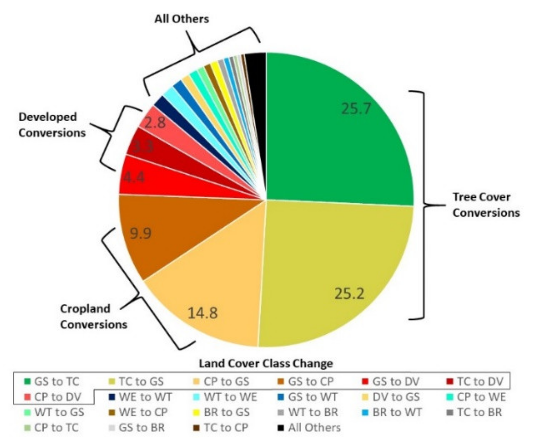
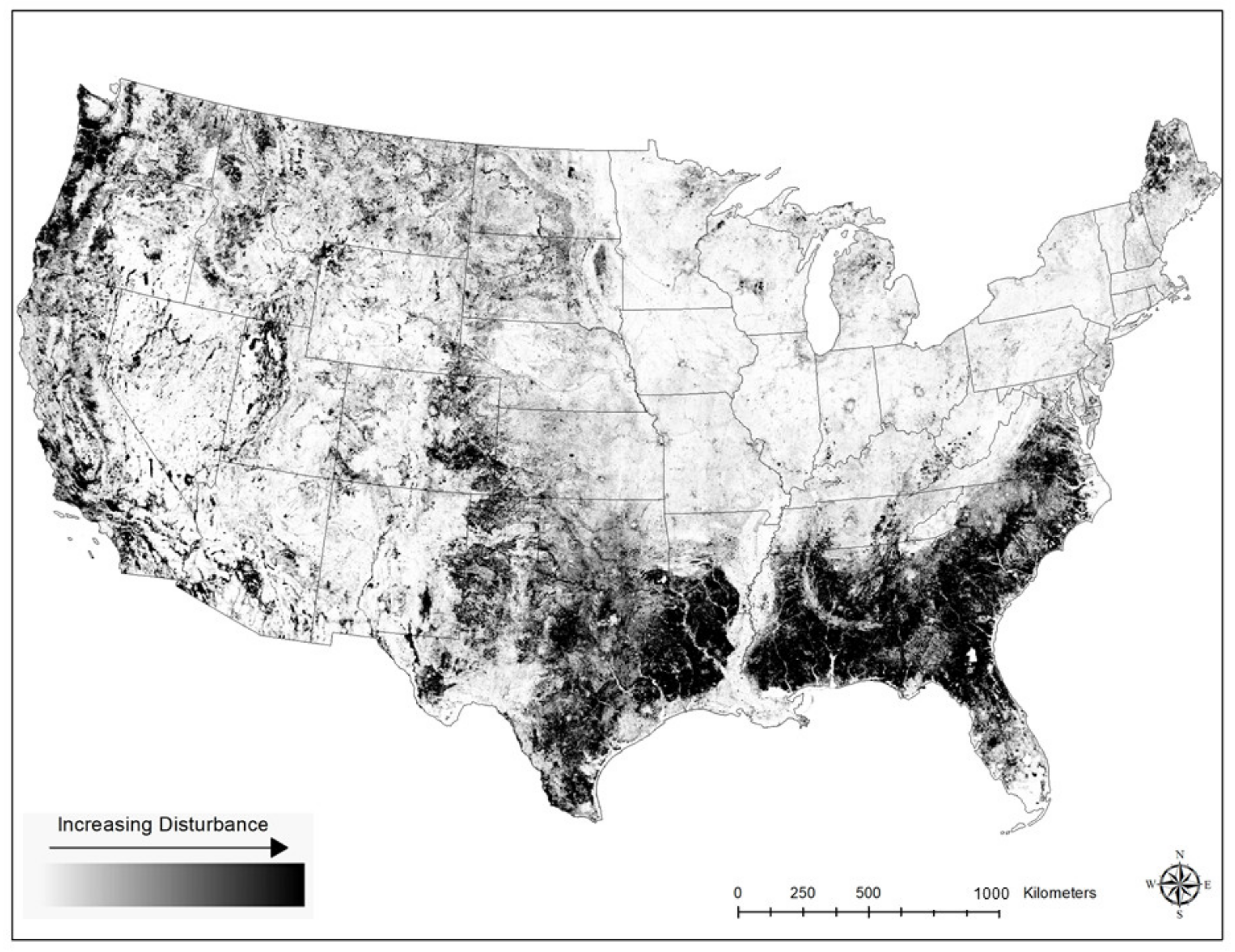
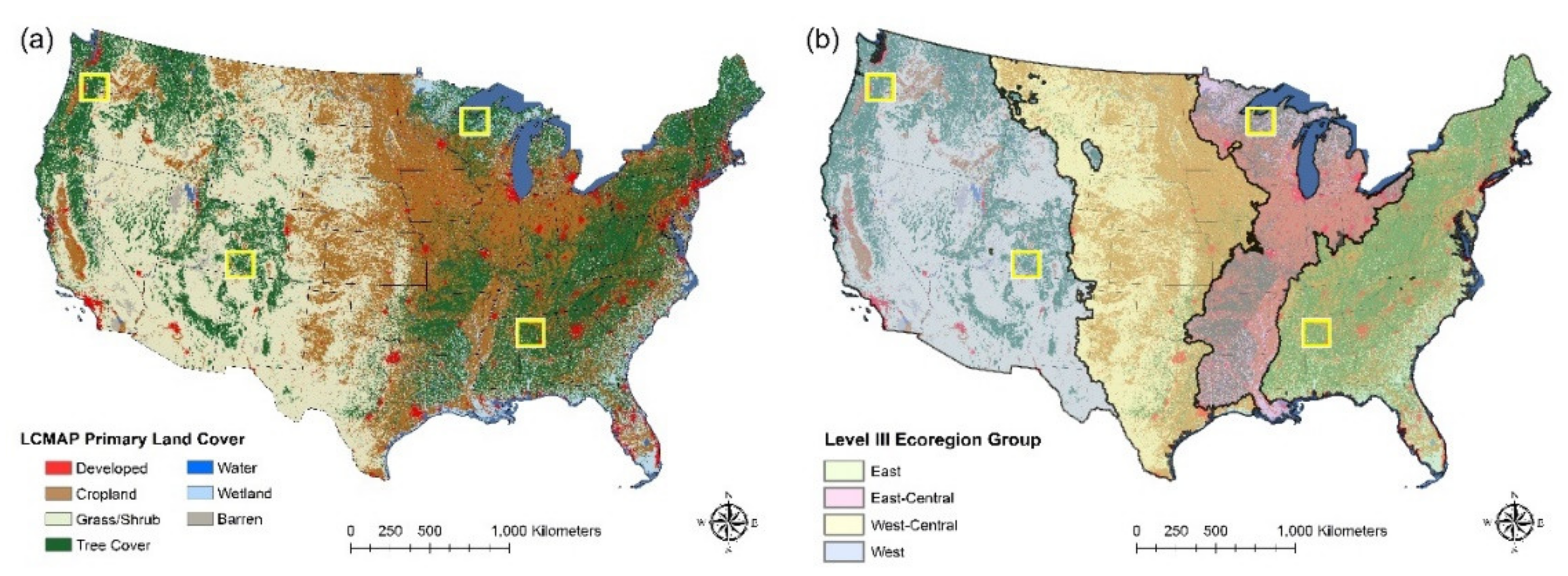
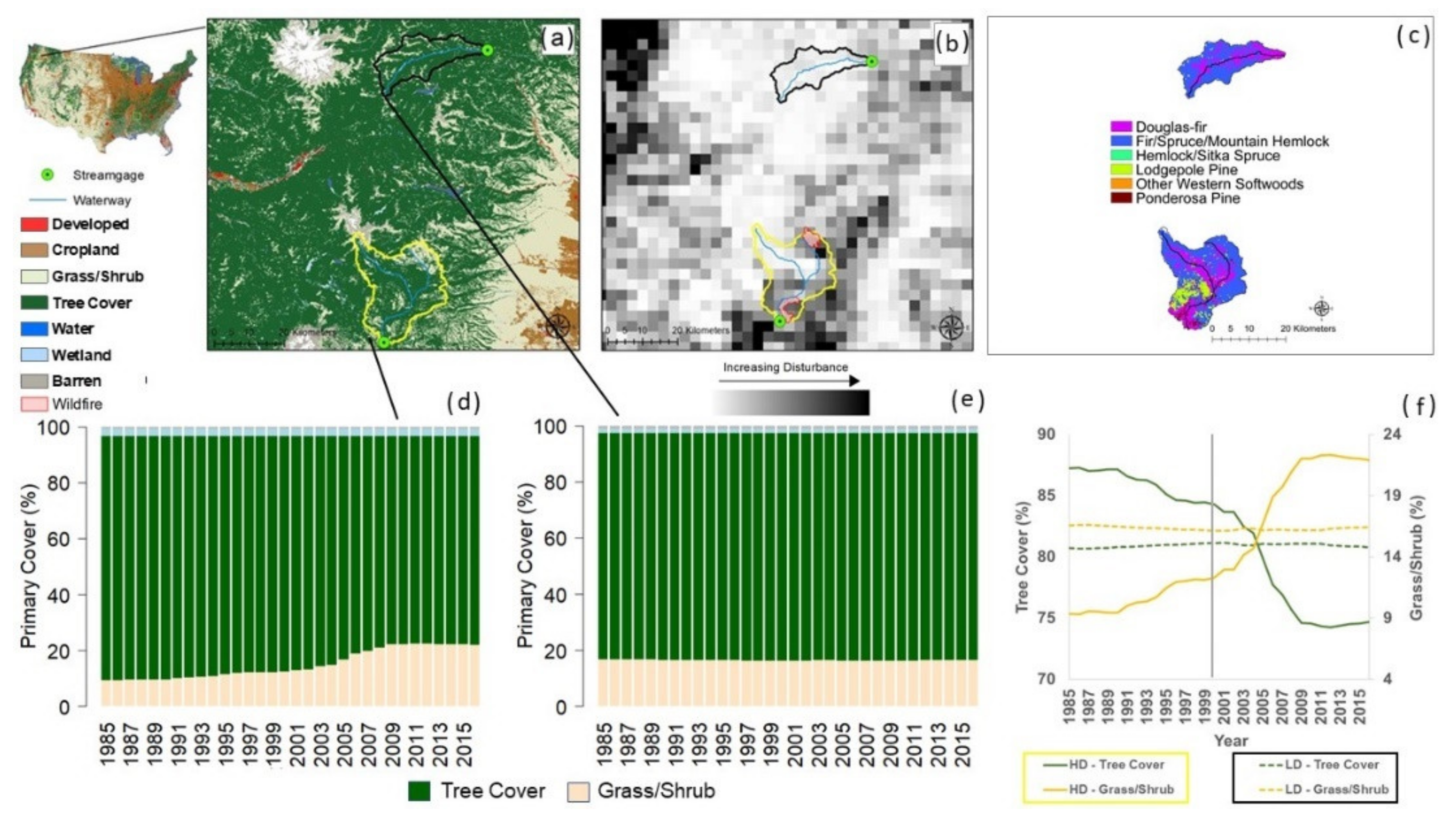
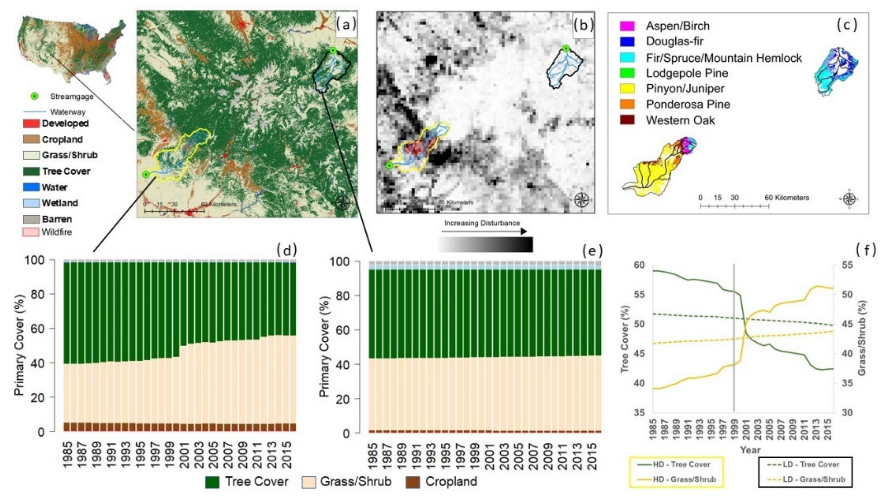
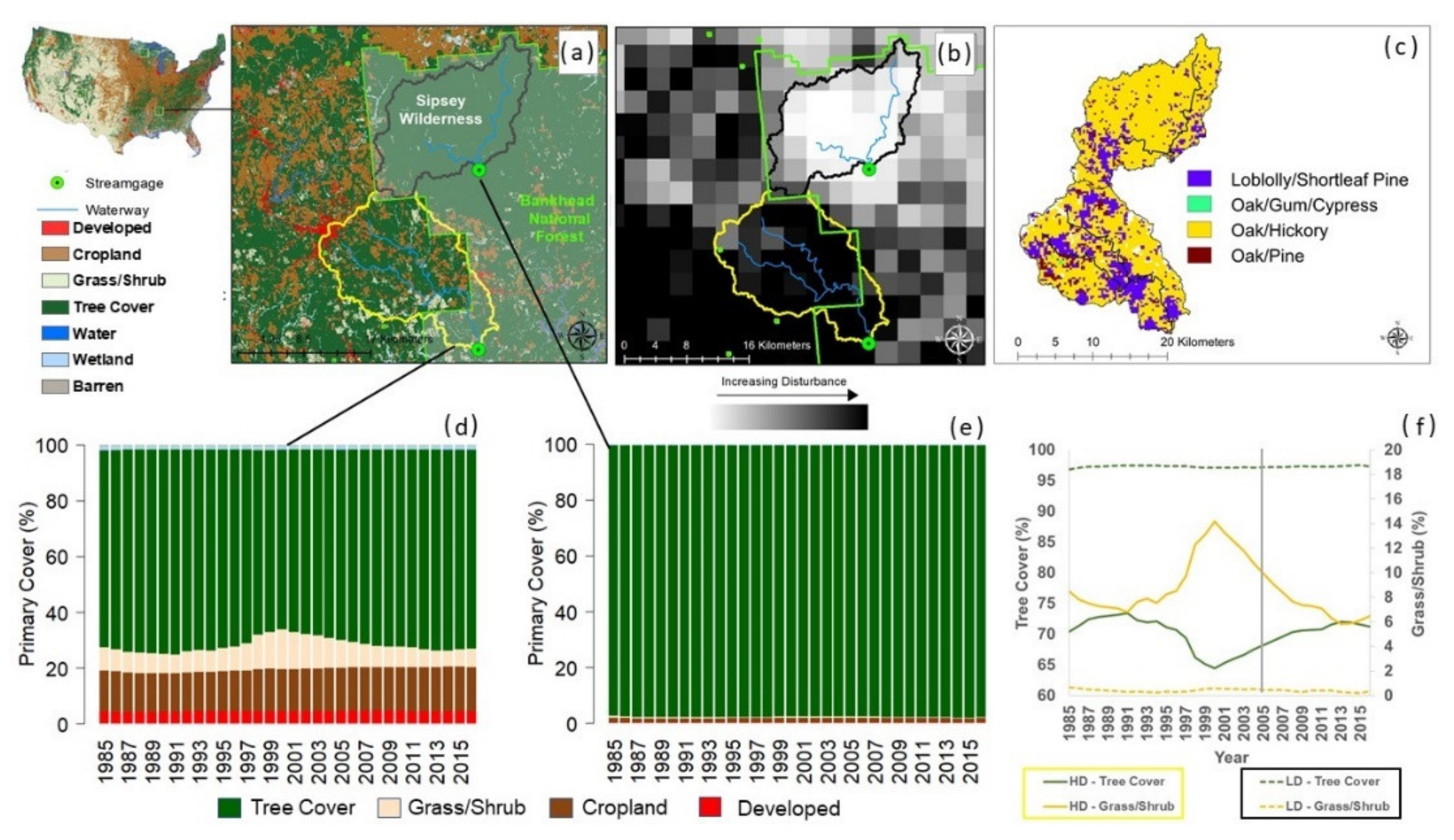
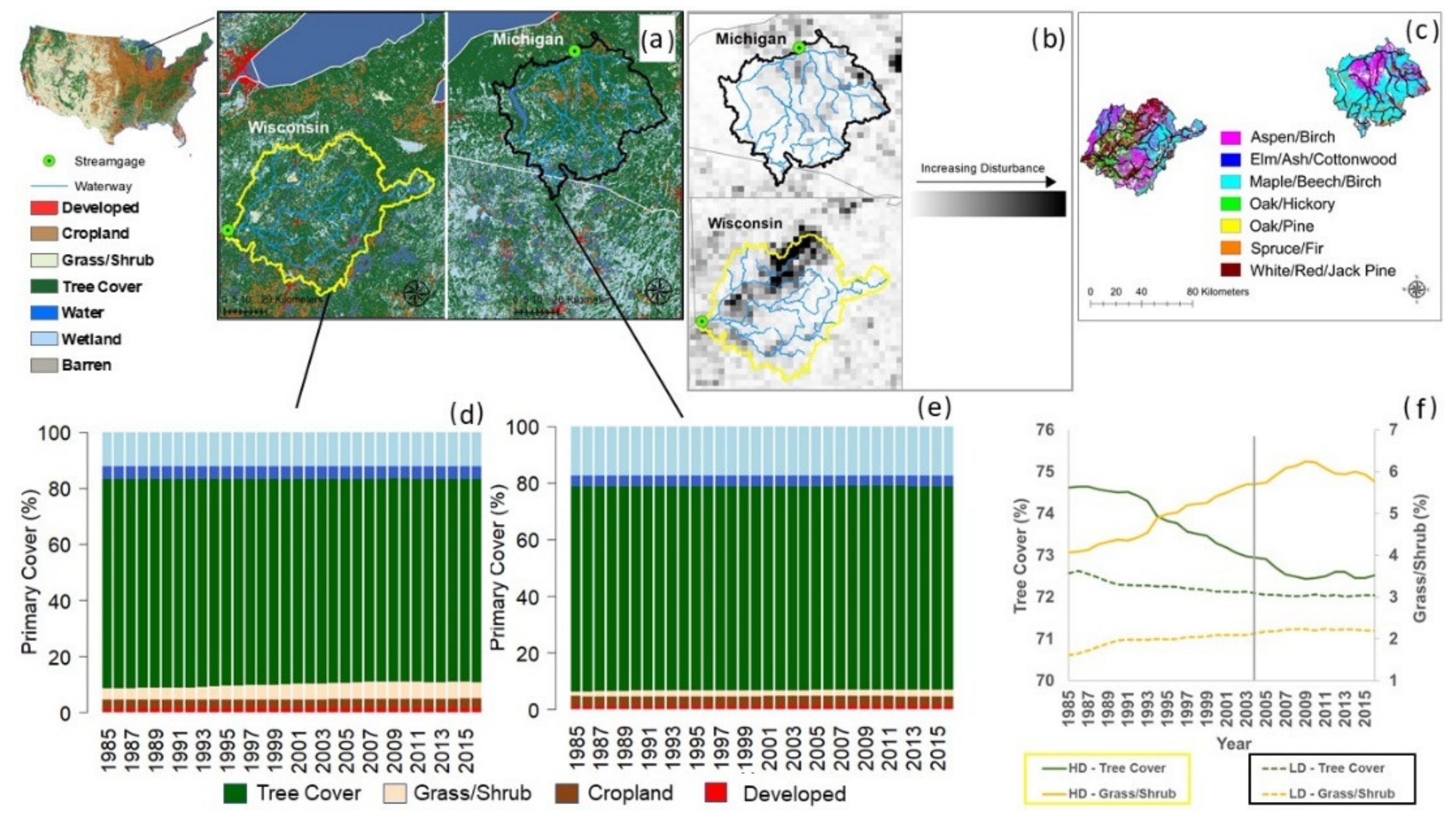
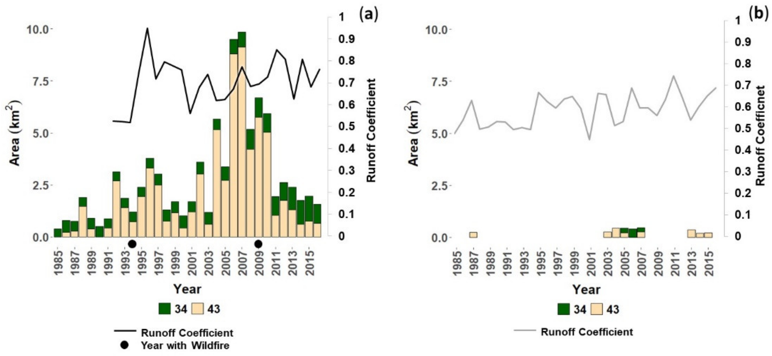
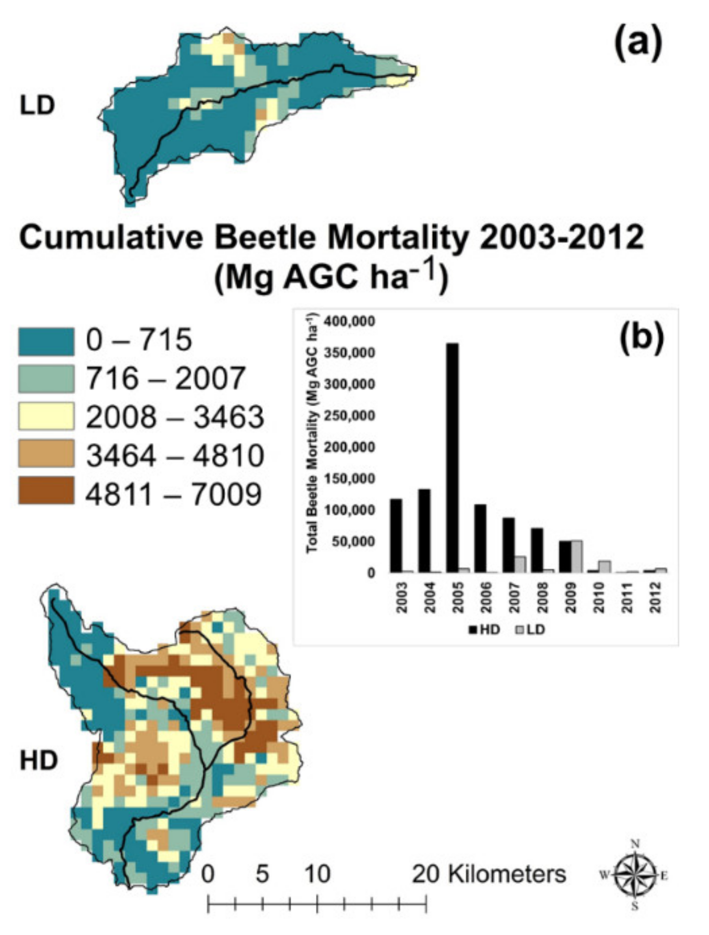
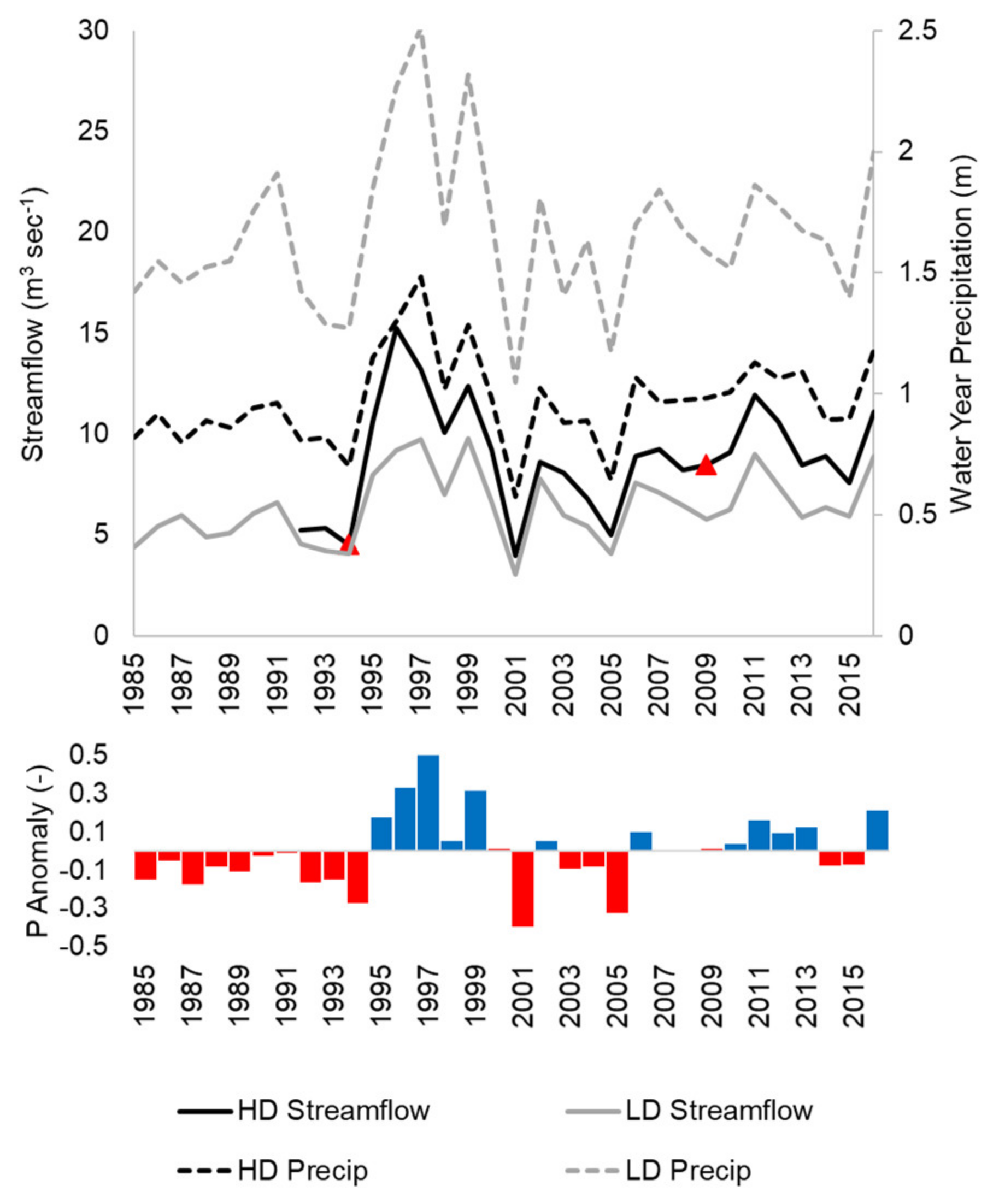
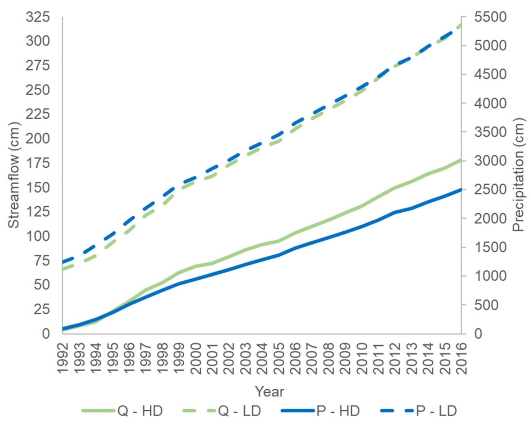
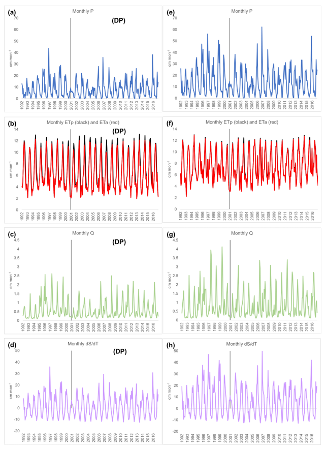
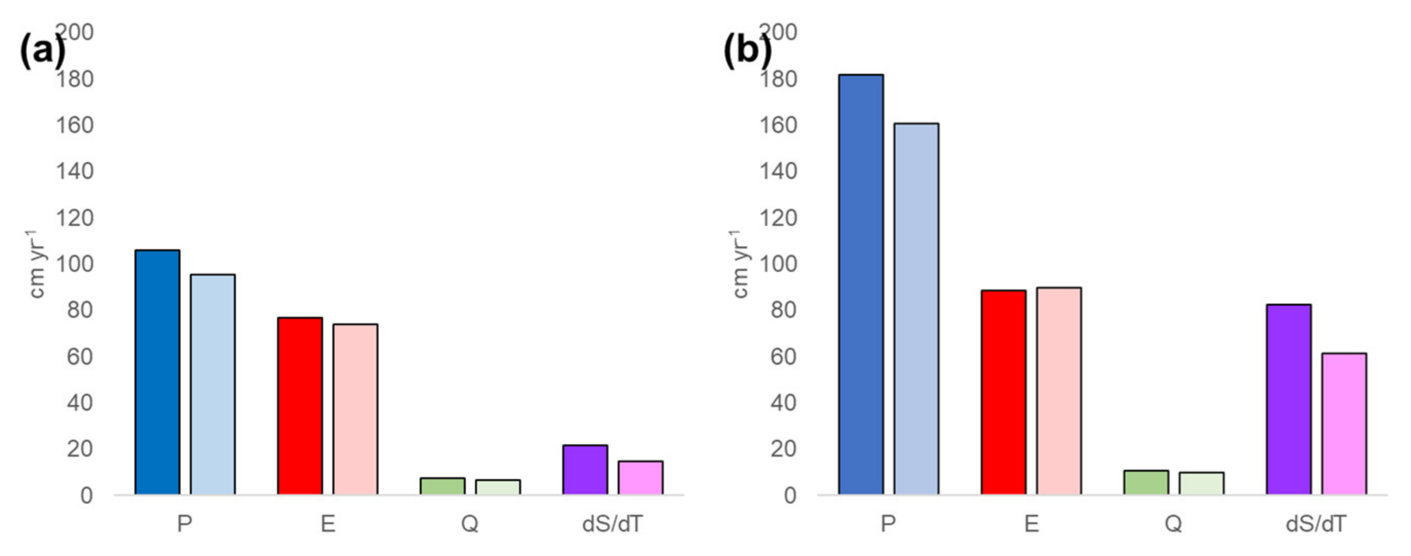
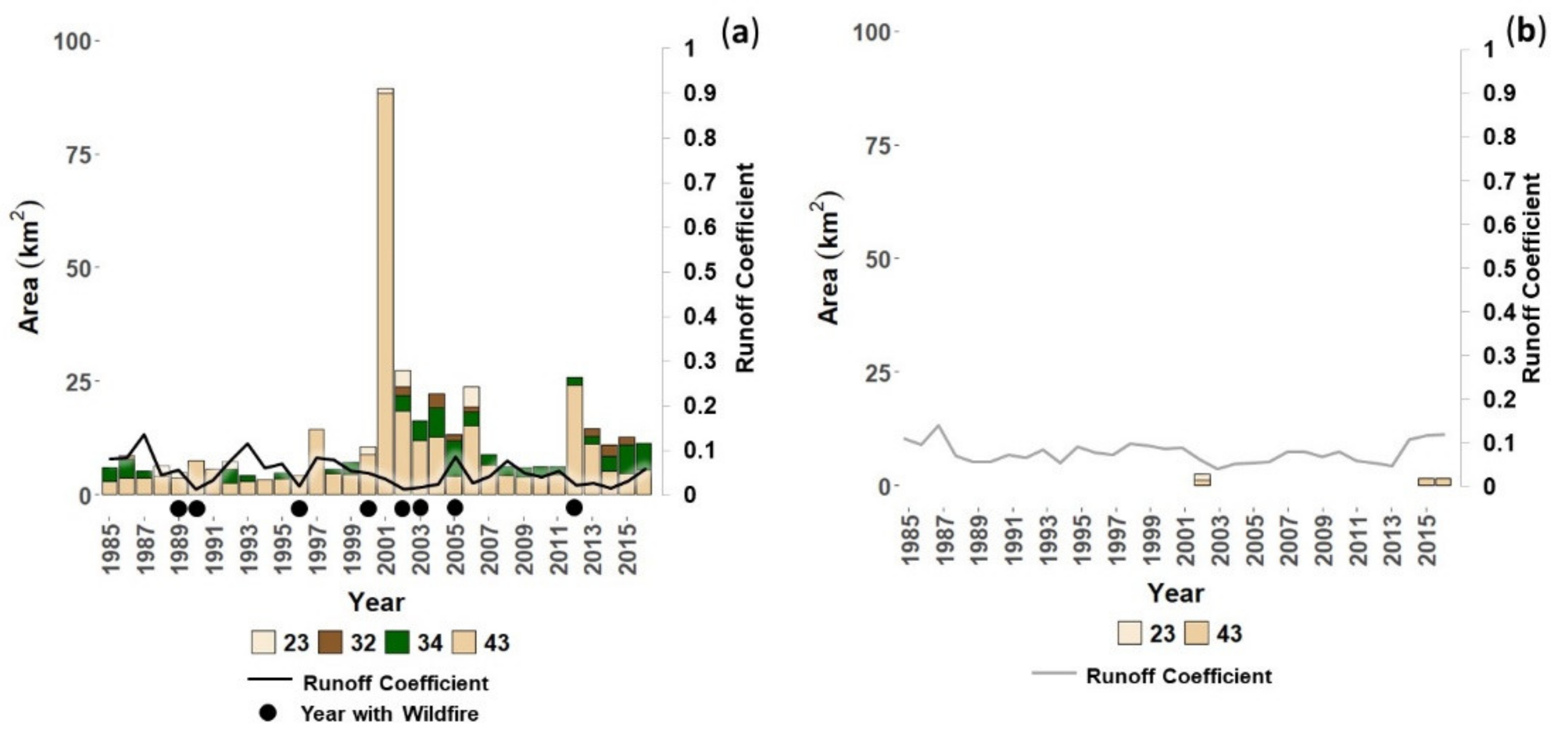
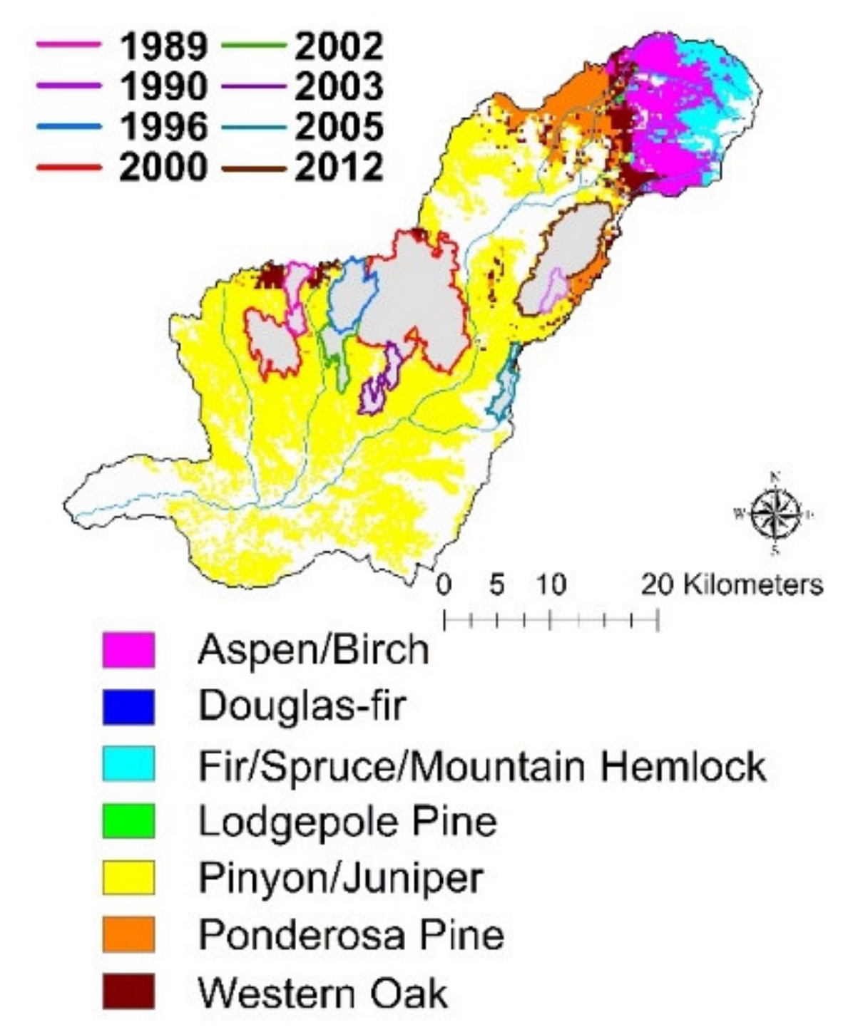
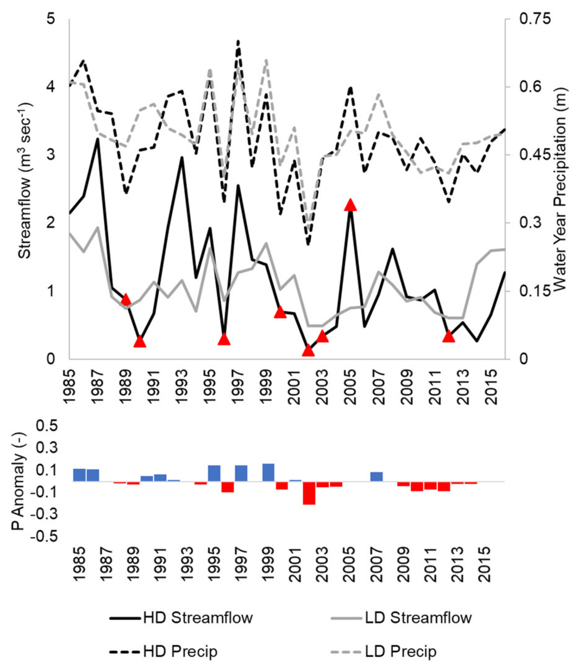
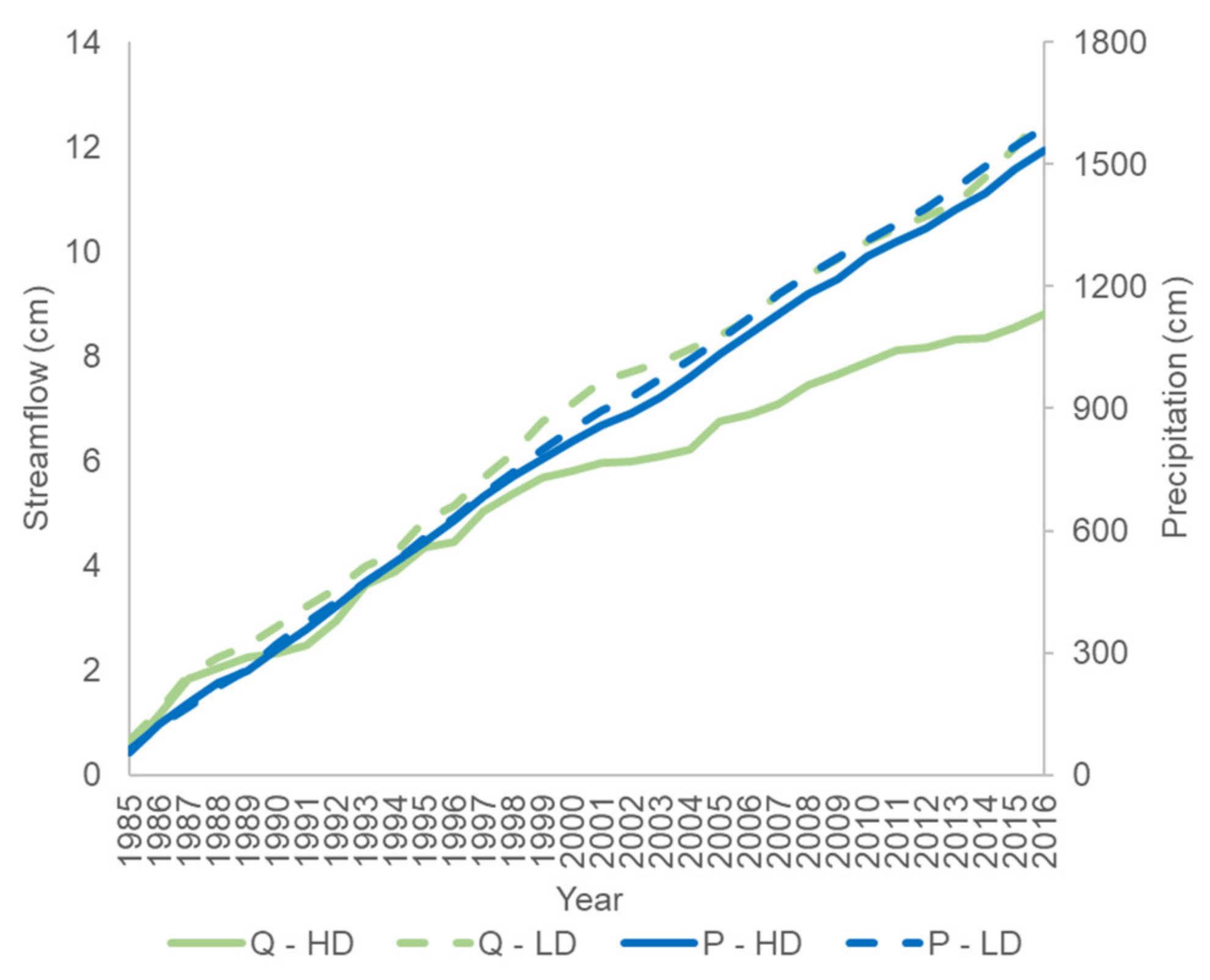
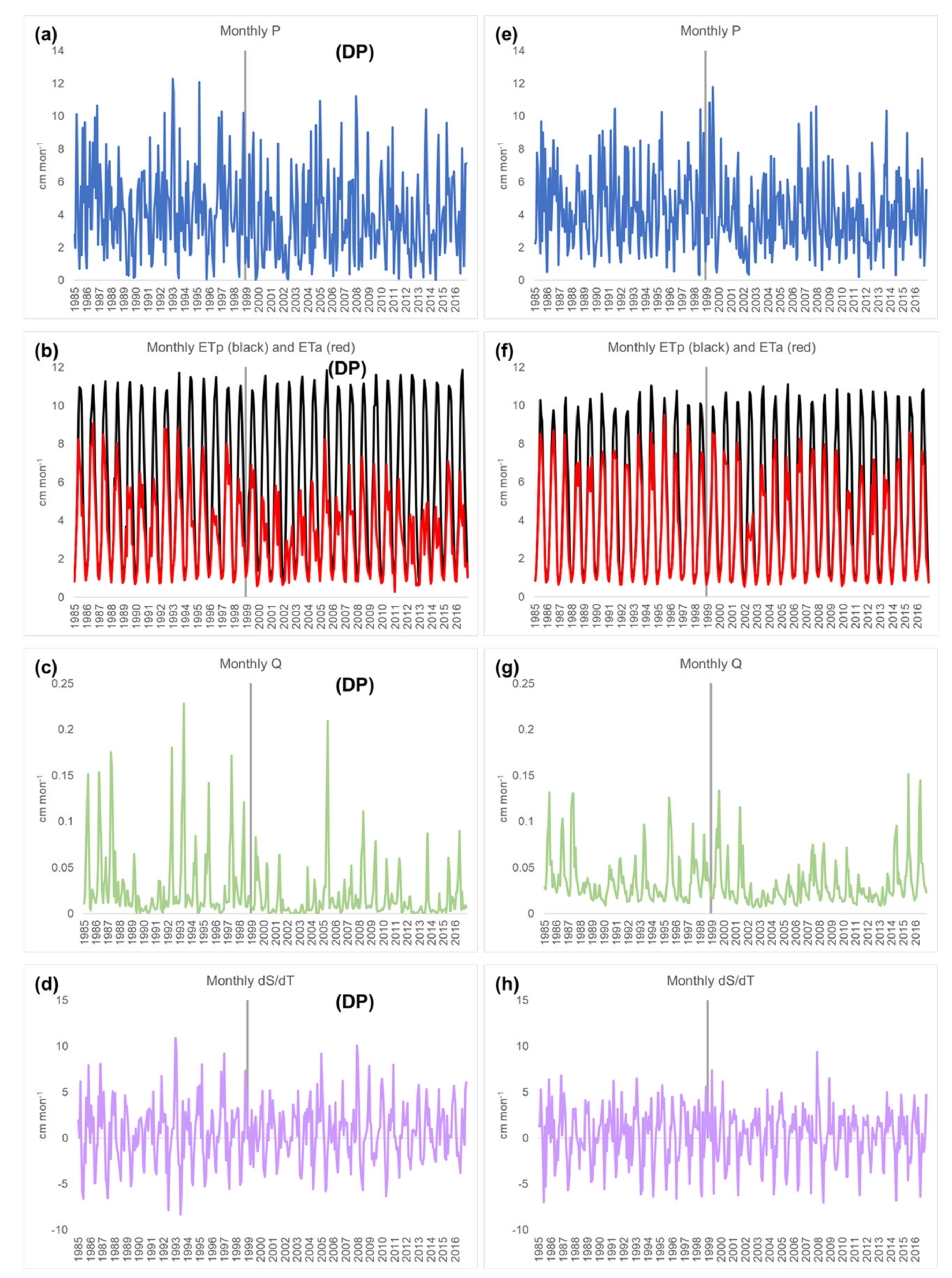
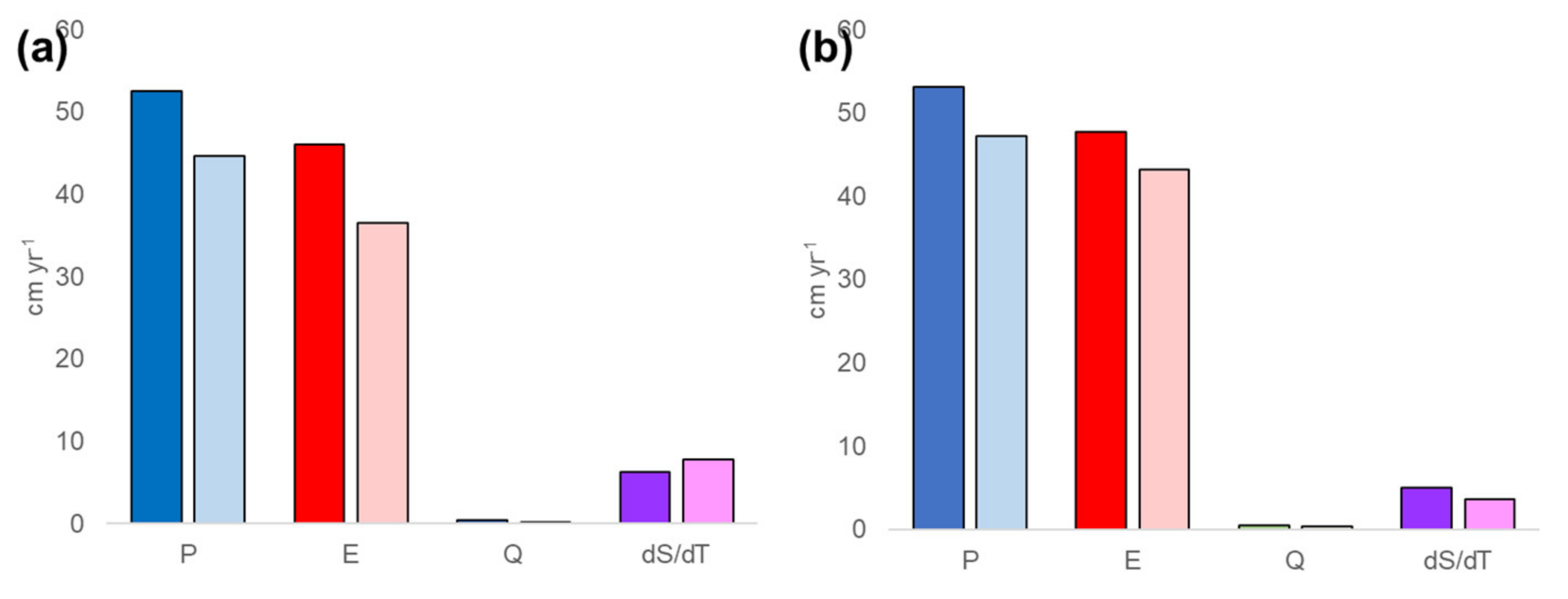
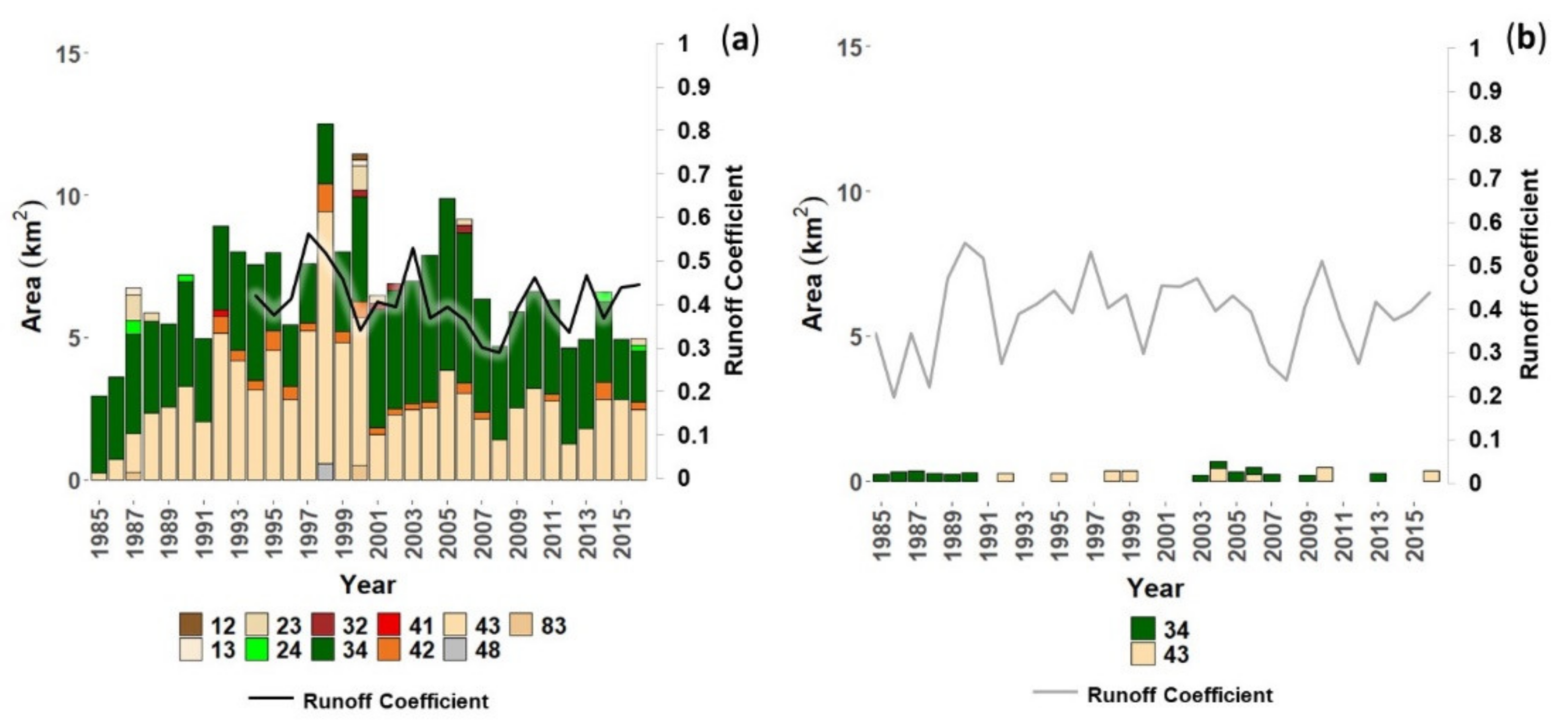
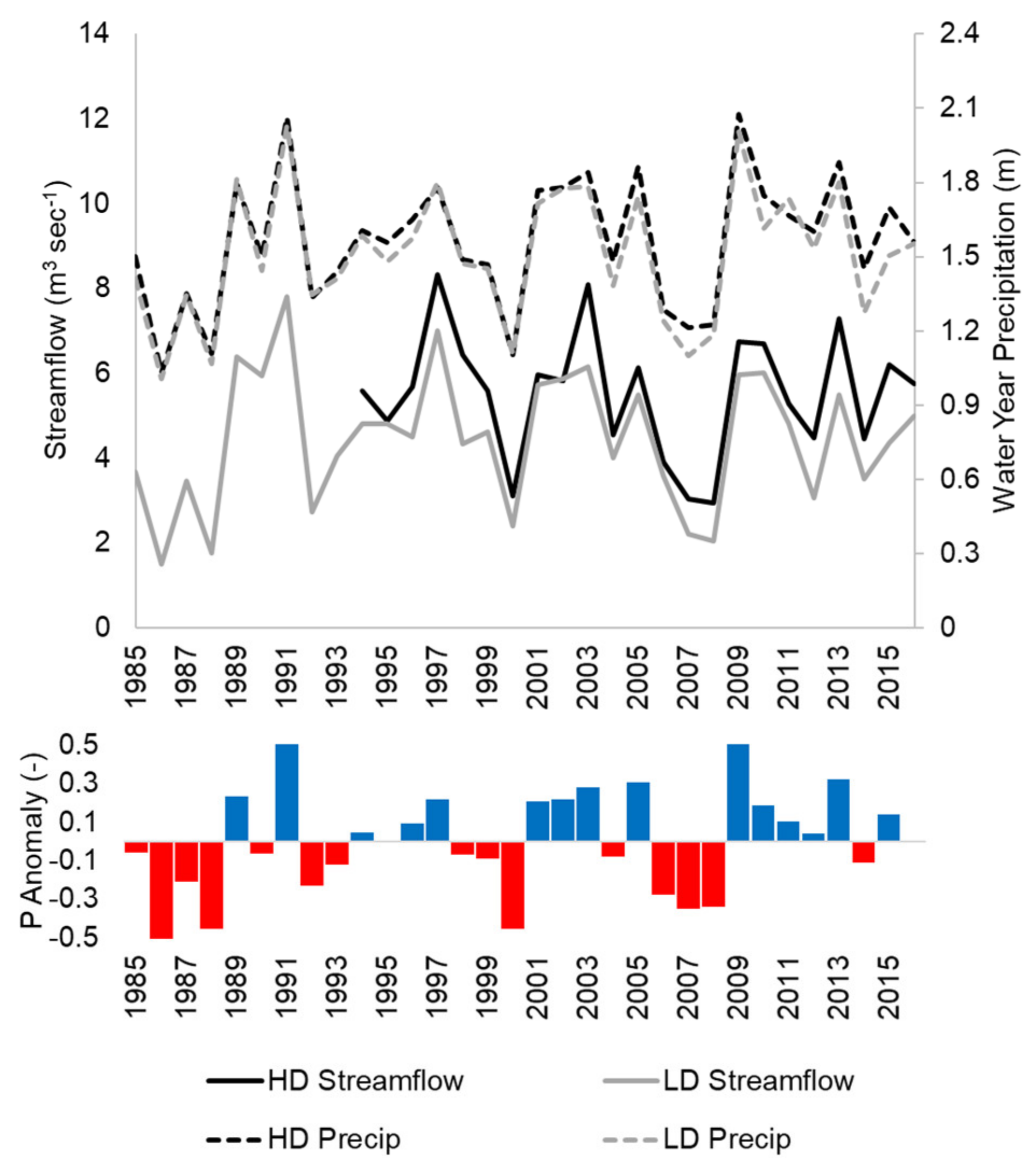
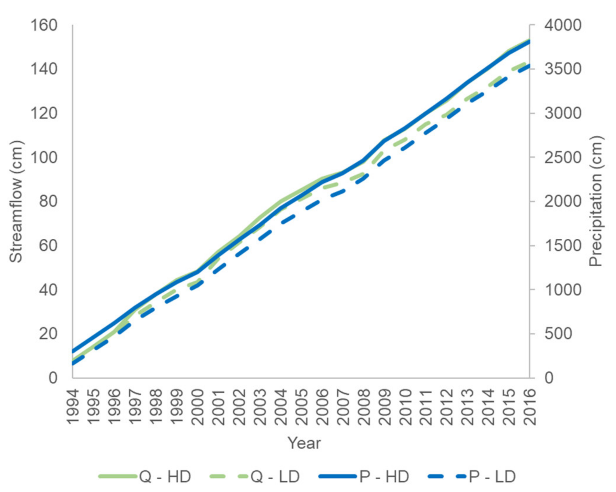
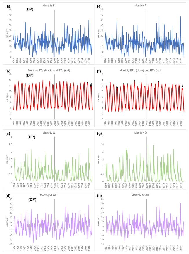
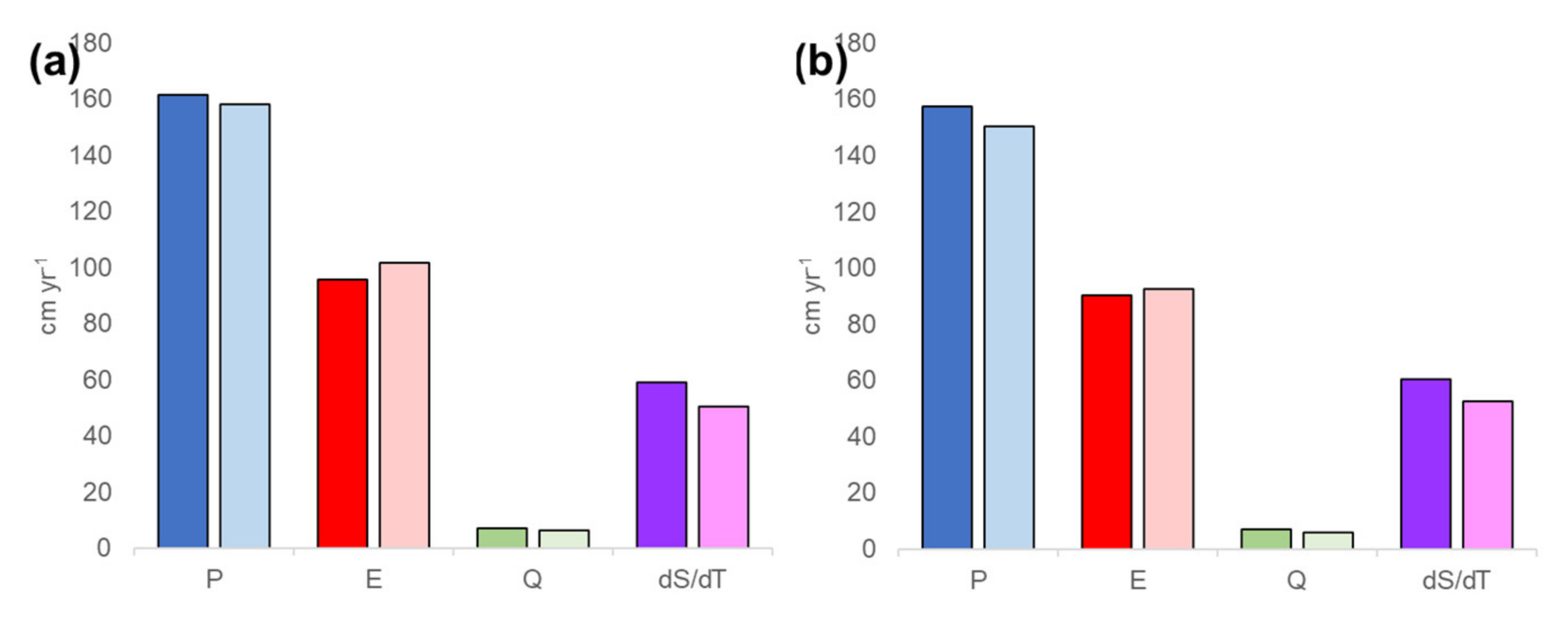
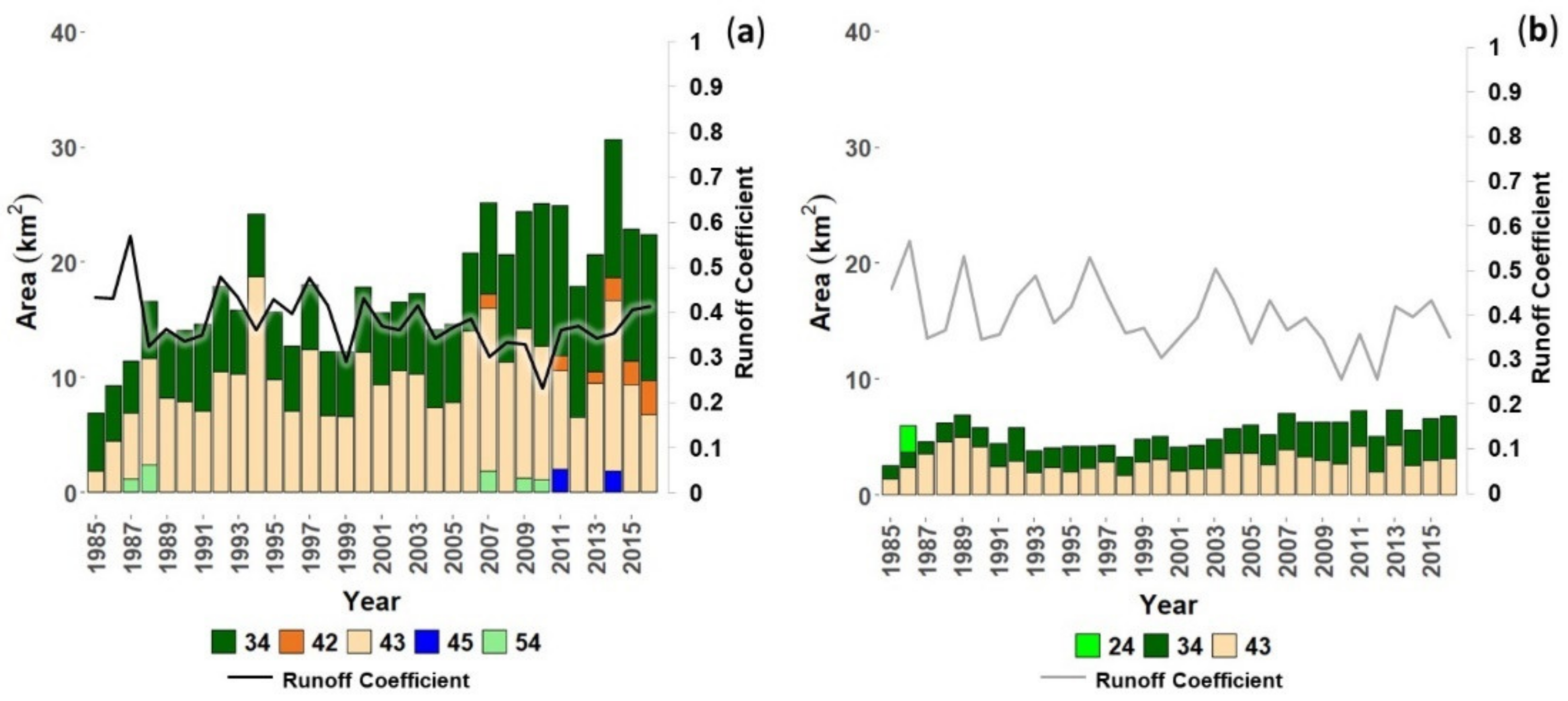
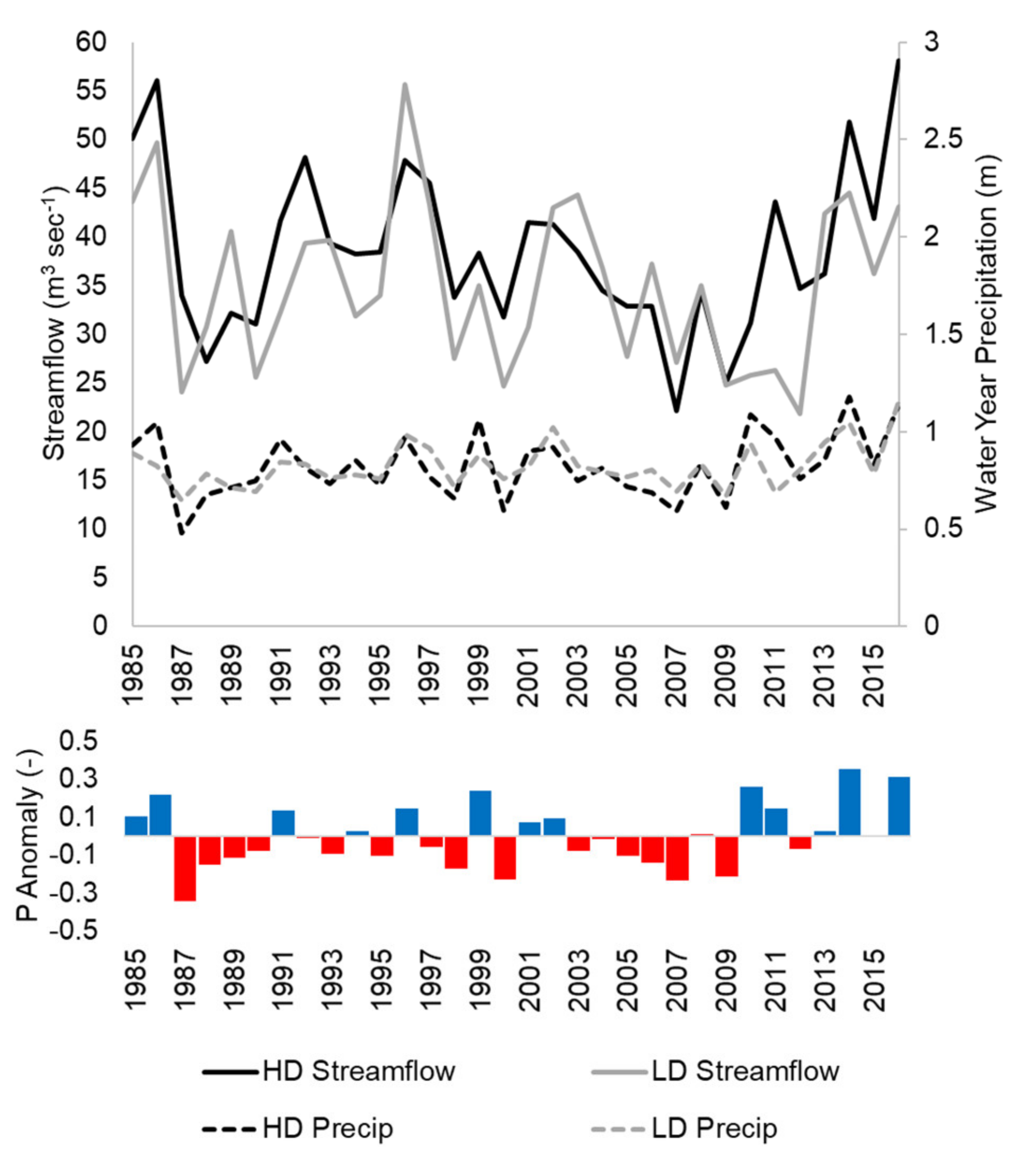
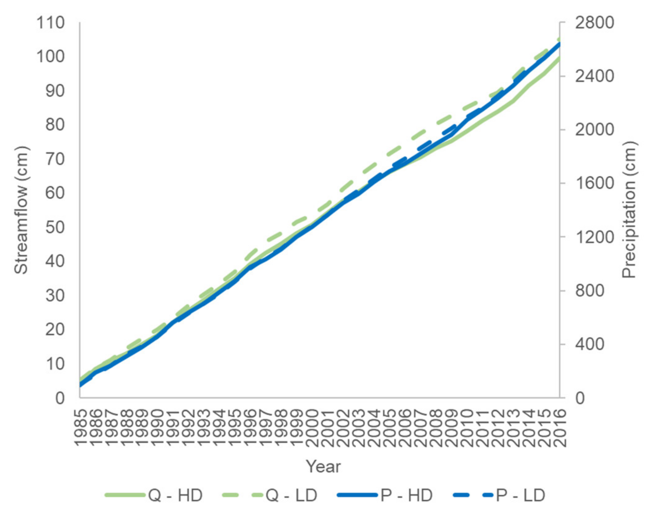
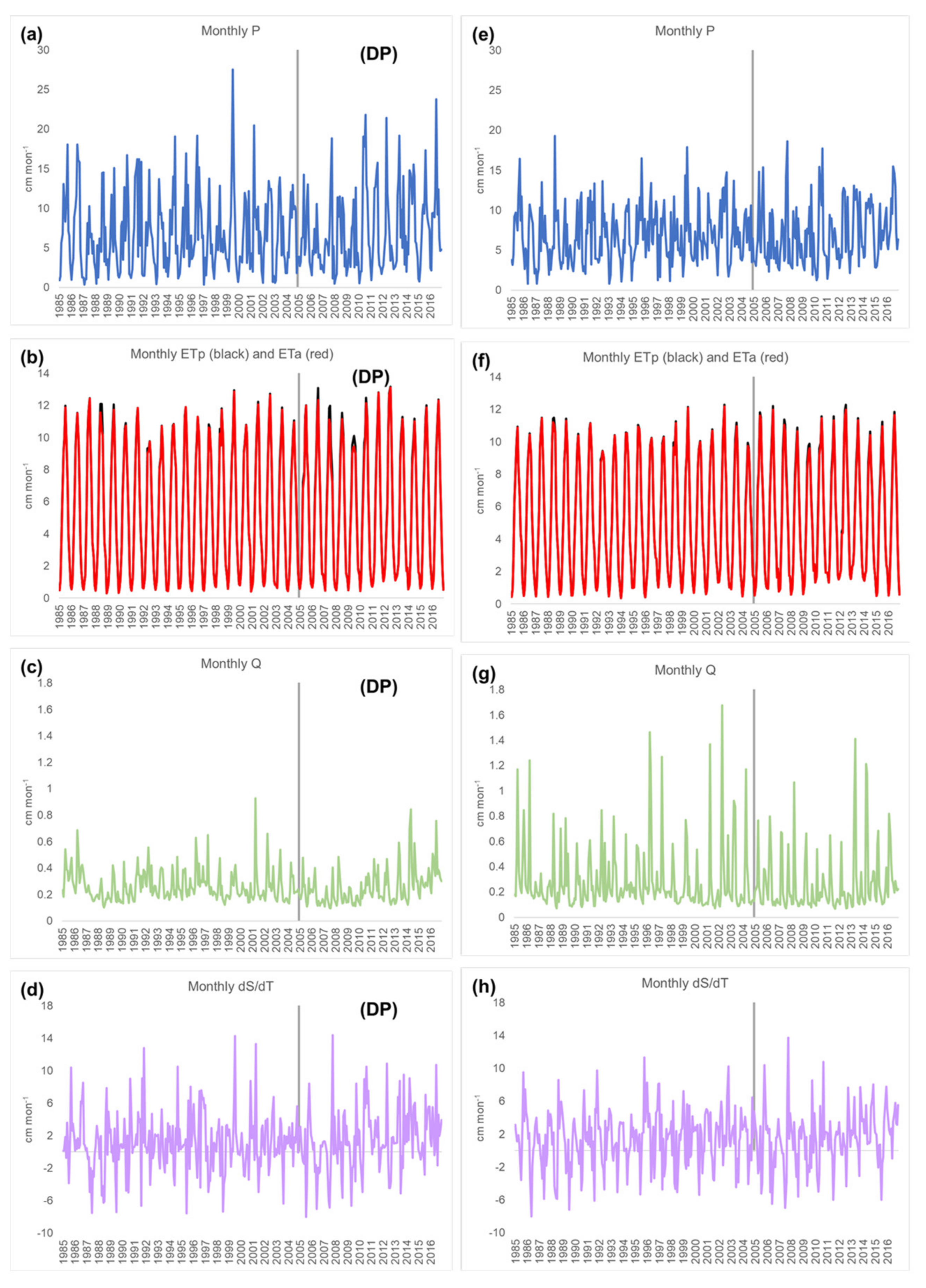
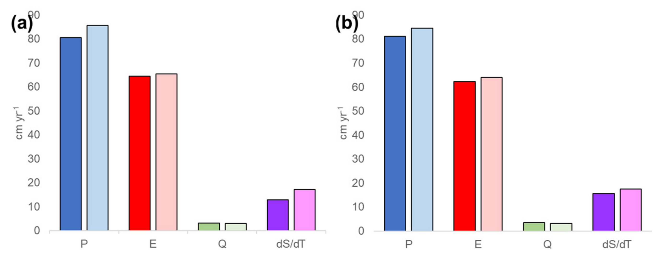
Table 1.
USGS streamgage information for all watersheds in this study. High-disturbance and low-disturbance watersheds are identified with HD and LD, respectively [50].
Table 1.
USGS streamgage information for all watersheds in this study. High-disturbance and low-disturbance watersheds are identified with HD and LD, respectively [50].
| State | USGS Streamgage | Latitude | Longitude | Area (km2) | Data Range | Missing Data |
|---|---|---|---|---|---|---|
| Washington (HD) | 14107000 | 46°15′54″ | 121°14′38″ | 391.34 | 1992–2020 | 1985–1991 |
| Washington (LD) | 12488500 | 46°58′40″ | 121°10′03″ | 205.22 | 1985–2020 | None |
| Colorado (HD) | 09371000 | 37°01′39″ | 108°44′27″ | 1353.00 | 1985–2020 | None |
| Colorado (LD) | 09118450 | 38°20′14″ | 106°46′25″ | 864.41 | 1985–2020 | None |
| Wisconsin (HD) | 05333500 | 46°04′34″ | 92°14′48″ | 3910.30 | 1985–2020 | None |
| Michigan (LD) | 04040000 | 46°43′15″ | 89°12′25″ | 3373.71 | 1985–2020 | None |
| Alabama (HD) | 02450825 | 34°04′52″ | 87°25′22″ | 262.05 | 1994–2020 | 1985–1993 |
| Alabama (LD) | 02450250 | 34°17′07″ | 87°23′56″ | 231.34 | 1985–2020 | None |
Table 2.
Details of watershed pairs [55,56,57] Precipitation represents annual average values from 1972 to 2000 [46,47,48,49]. Streamflow represents average annual values from 1985 to 2016 [50].
| State | Watershed | Level II Ecoregion | Level III Ecoregion(s) | Soil Textures | Annual Average Precipitation | Average Annual Streamflow | Main Disturbance(s) |
|---|---|---|---|---|---|---|---|
| (mm) | (m3 s−1) | ||||||
| Washington (HD) | Klickitat River | Western Cordillera | 75% Eastern Cascades Slopes and Foothills, 25% Cascades | Loam, silt loam, clay loam, cobbly loam, stony loam, stony silt loam, and sandy loam. | 500–3000 | 8.8 | Insect Infestation, Wildfire |
| Washington (LD) | American River | Western Cordillera | 25% Eastern Cascades Slopes and Foothills, 75% Cascades | Loam, silt loam, cobbly loam, stony loam, stony silt loam, and sandy loam. | 500–3000 | 6.4 | None |
| Colorado (HD) | Mancos River | Western Cordillera/Cold Deserts | 80% Colorado Plateaus, 20% Southern Rockies | Sand, sandy loam, cobbly loam, and ashy loam | 250–1000 | 1.2 | Wildfire |
| Colorado (LD) | Cochetopa Creek | Western Cordillera/Cold Deserts | Southern Rockies | Stony loam, sandy loam, and gravelly loam. | 250–1000 | 1.1 | None |
| Alabama (HD) | Clear Creek | Ozark/Ouachita-Appalachian Forest | Southwestern Appalachian | Shaley silt loam, sandy loam, clay loam, silty clay loam, and silty clay. | 1000–2000 | 5.5 | Logging, Timber Harvest |
| Alabama (LD) | Sipsy Fork | Ozark/Ouachita-Appalachian Forest | Southwestern Appalachian | Shaley silt loam, sandy loam, clay loam, silty clay loam, and silty clay. | 1000–2000 | 4.5 | None |
| Wisconsin (HD) | St. Croix and Namekagon Rivers | Mixed Wood Shield | Northern Lakes and Forests | Sand, sandy loam, cobbly loam, loam, and peat. | 600–900 | 38.6 | Logging, Timber Harvest |
| Michigan (LD) | Ontonagon River | Mixed Wood Shield | Northern Lakes and Forests | Sand, sandy loam, cobbly loam, loam, clay, peat, muck, and silt. | 600–900 | 35.1 | None |
Table 3.
Forest group types of each disturbed watershed [44].
Table 3.
Forest group types of each disturbed watershed [44].
| State | Watershed | Forest Group Types |
|---|---|---|
| Washington (HD) | Klickitat River | 58% fir/spruce/mountain hemlock (Abies spp., Picea spp., and Tsuga spp., respectively); |
| 27% Douglas-fir (Pseudotsuga menziesii); | ||
| 12% lodgepole pine (Pinus contorta); | ||
| 3% ponderosa pine (Pinus ponderosa). | ||
| Washington (LD) | American River | 70% fir/spruce/mountain hemlock (Abies spp., Picea spp., and Tsuga mertensiana, respectively); |
| 30% Douglas-fir (Pseudotsuga menziesii). | ||
| Colorado (HD) | Mancos River | 71% pinyon-juniper woodland (Pinus spp., and Juniperus spp.) |
| 9% oak (Quercus spp.); | ||
| 8% aspen and birch (Populus tremuloides and Betula spp.); | ||
| 7% ponderosa pine (Pinus ponderosa); | ||
| 4% fir/spruce/mountain hemlock (Abies spp., Picea spp., and Tsuga mertensiana, respectively). | ||
| Colorado (LD) | Cochetopa Creek | 61% fir/spruce/mountain hemlock (Abies spp., Picea spp., and Tsuga mertensiana, respectively); |
| 26% Douglas-fir (Pseudotsuga menziesii); | ||
| 10% aspen and birch (Populus tremuloides and Betula spp.); | ||
| 3% lodgepole pine (Pinus contorta). | ||
| Alabama (HD) | Clear Creek | 65% an oak and hickory (Quercus spp. and Carya spp., respectively); |
| 30% loblolly pine and shortleaf pine (Pinus taeda and Pinus echinate, respectively); | ||
| 5% oak and pine group (Quercus spp. and Pinus spp., respectively). | ||
| Alabama (LD) | Sipsy Fork | 84% an oak and hickory (Quercus spp. and Carya spp., respectively); |
| 13% loblolly pine and shortleaf pine (Pinus taeda and Pinus echinate, respectively); | ||
| 3% oak and pine (Quercus spp. and Pinus spp., respectively). | ||
| Wisconsin (HD) | St. Croix and Namekagon Rivers | 31% aspen and birch group (Populus tremuloides and Betula spp., respectively); |
| 24% white pine, red pine, and jack pine group (Pinus strobus, Pinus resinosa, and Pinus banksiana Lamb., respectively); | ||
| 23% maple, beech, and birch group (Acer spp., Fagus spp., and Betula spp., respectively); | ||
| 4% spruce and fir (Picea spp. and Abies spp., respectively); | ||
| 3% elm, ash, and cottonwood group (Ulmus spp., Fraxinus spp., and Populus deltoides). | ||
| Michigan (LD) | Ontonagon River | 62% maple, beech, and birch group (Acer spp., Fagus spp., and Betula spp., respectively); |
| 26% aspen and birch group (Populus tremuloides and Betula spp., respectively) | ||
| 3% white pine, red pine, and jack pine group (Pinus strobus, Pinus resinosa, and Pinus banksiana Lamb., respectively); | ||
| 8% spruce and fir group (Picea spp. and Abies spp., respectively). |
Table 4.
Average annual water year water balance (P: precipitation, E: evaporation, Q: outflow, dS/dT: storage change) for the Washington watershed pair during the stable period (SP) and the disturbed period (DP).
Table 4.
Average annual water year water balance (P: precipitation, E: evaporation, Q: outflow, dS/dT: storage change) for the Washington watershed pair during the stable period (SP) and the disturbed period (DP).
| Watershed | P | E | Q | dS/dT | ||
|---|---|---|---|---|---|---|
| (cm year−1) | (cm year−1) | (cm year−1) | (cm year−1) | |||
| Washington-HD | SP | 1992–2000 | 106.1 | 76.7 | 7.7 | 21.8 |
| Klickitat River | DP | 2001–2016 | 95.4 | 73.9 | 6.8 | 14.8 |
| Difference | cm year−1 (%) | −10.6 (−10.0) | −2.8 (−3.6) | −0.9 (−11.3) | −7.0 (−32.1) | |
| Washington-LD | SP | 1992–2000 | 181.6 | 88.4 | 10.8 | 82.4 |
| American River | DP | 2001–2016 | 160.9 | 89.6 | 9.9 | 61.4 |
| Difference | cm year−1 (%) | −20.7 (−11.4) | 1.2 (1.4) | −0.9 (−8.2) | −21.1 (−25.5) |
Table 5.
Average annual water year water balance (P: precipitation, E: evaporation, Q: outflow, dS/dT: storage change) for the Colorado watershed pair during the stable period (SP) and the disturbed period (DP).
Table 5.
Average annual water year water balance (P: precipitation, E: evaporation, Q: outflow, dS/dT: storage change) for the Colorado watershed pair during the stable period (SP) and the disturbed period (DP).
| Watershed | P | E | Q | dS/dT | ||
|---|---|---|---|---|---|---|
| (cm year−1) | (cm year−1) | (cm year−1) | (cm year−1) | |||
| Colorado-HD | SP | 1985–1998 | 52.6 | 46.0 | 0.4 | 6.2 |
| Mancos River | DP | 1999–2016 | 44.6 | 36.6 | 0.2 | 7.8 |
| Difference | cm year−1 (%) | −8.0 (−15.2) | −9.4 (−20.5) | −0.2 (−49.5) | 1.6 (26.3) | |
| Colorado-LD | SP | 1985–1998 | 53.1 | 47.7 | 0.4 | 5.0 |
| Cochetopa Creek | DP | 1999–2016 | 47.3 | 43.3 | 0.4 | 3.6 |
| Difference | cm year−1 (%) | −5.8 (−11.1) | −4.4 (−9.3) | −0.1 (−18.3) | −1.4 (−27.1) |
Table 6.
Average annual water year water balance (P: precipitation, E: evaporation, Q: outflow, dS/dT: storage change) for the Alabama watershed pair during the stable period (SP) and the disturbed period (DP).
Table 6.
Average annual water year water balance (P: precipitation, E: evaporation, Q: outflow, dS/dT: storage change) for the Alabama watershed pair during the stable period (SP) and the disturbed period (DP).
| Watershed | P | E | Q | dS/dT | ||
|---|---|---|---|---|---|---|
| (cm year−1) | (cm year−1) | (cm year−1) | (cm year−1) | |||
| Alabama-HD | DP | 1994–2005 | 161.6 | 95.5 | 7.0 | 59.1 |
| Clear Creek | SP | 2006–2016 | 158.2 | 101.5 | 6.2 | 50.5 |
| Difference | cm year−1 (%) | −3.4 (−2.1) | 6.0 (6.3) | −0.8 (−11.8) | −8.6 (−14.5) | |
| Alabama-LD | DP | 1994–2005 | 157.3 | 90.2 | 6.8 | 60.3 |
| Sipsey Fork | SP | 2006–2016 | 150.4 | 92.3 | 5.7 | 52.4 |
| Difference | cm year−1 (%) | −6.9 (−4.4) | 2.2 (2.4) | −1.1 (−15.9) | −7.9 (−13.2) |
Table 7.
Average annual water year water balance (P: precipitation, E: evaporation, Q: outflow, dS/dT: storage change) for the Wisconsin/Michigan watershed pair during the stable period (SP) and the disturbed period (DP).
Table 7.
Average annual water year water balance (P: precipitation, E: evaporation, Q: outflow, dS/dT: storage change) for the Wisconsin/Michigan watershed pair during the stable period (SP) and the disturbed period (DP).
| Watershed | P | E | Q | dS/dT | ||
|---|---|---|---|---|---|---|
| (cm year−1) | (cm year−1) | (cm year−1) | (cm year−1) | |||
| Wisconsin—HD | SP | 1985–2004 | 80.6 | 64.5 | 3.2 | 12.9 |
| St. Croix/ Namekagon Rivers | DP | 2005–2016 | 85.6 | 65.3 | 3.0 | 17.3 |
| Difference | cm year−1 (%) | 5.0 (6.2) | 0.8 (1.3) | −0.2 (−6.1) | 4.4 (34.2) | |
| Michigan—LD | SP | 1985–2004 | 81.2 | 62.2 | 3.4 | 15.6 |
| Ontonagon River | DP | 2005–2016 | 84.4 | 63.9 | 3.1 | 17.4 |
| Difference | cm year−1 (%) | 3.2 (4.0) | 1.7 (2.8) | −0.4 (−10.8) | 1.9 (12.0) |
Publisher’s Note: MDPI stays neutral with regard to jurisdictional claims in published maps and institutional affiliations. |
© 2022 by the authors. Licensee MDPI, Basel, Switzerland. This article is an open access article distributed under the terms and conditions of the Creative Commons Attribution (CC BY) license (https://creativecommons.org/licenses/by/4.0/).
Share and Cite
MDPI and ACS Style
Healey, N.C.; Rover, J.A. Analyzing the Effects of Land Cover Change on the Water Balance for Case Study Watersheds in Different Forested Ecosystems in the USA. Land 2022, 11, 316. https://0-doi-org.brum.beds.ac.uk/10.3390/land11020316
AMA Style
Healey NC, Rover JA. Analyzing the Effects of Land Cover Change on the Water Balance for Case Study Watersheds in Different Forested Ecosystems in the USA. Land. 2022; 11(2):316. https://0-doi-org.brum.beds.ac.uk/10.3390/land11020316
Chicago/Turabian StyleHealey, Nathan C., and Jennifer A. Rover. 2022. "Analyzing the Effects of Land Cover Change on the Water Balance for Case Study Watersheds in Different Forested Ecosystems in the USA" Land 11, no. 2: 316. https://0-doi-org.brum.beds.ac.uk/10.3390/land11020316
Note that from the first issue of 2016, this journal uses article numbers instead of page numbers. See further details here.