
Unravelling the Impacts of Climate Variability on Surface Runoff in the Mouhoun River Catchment (West Africa)


1
Laboratoire de Physique et Chimie de l’Environnement (LPCE), Institut de Génie de l’Environnement et du Développement Durable (IGEDD), Université Joseph KI-ZERBO (UJKZ), Ouagadougou 03 BP 7021, Burkina Faso
2
Service Régional des Etudes Statistiques et Sectorielles, Direction Régionale de l’Eau et de l’Assainissement du Centre-Nord, Ministère de l’Environnement, de l’Eau et de l’Assainissement, Ouagadougou 03 BP 7044, Burkina Faso
3
Laboratoire Eaux, Hydro-Systèmes et Agriculture (LEHSA), Institut International d’Ingénierie de l’Eau et de l’Environnement (2iE), Ouagadougou 01 BP 594, Burkina Faso
4
Département Information et Recherche (DIR), Centre Climatique Régional pour l’Afrique de l’Ouest et le Sahel (CCR-WAS), Centre Régional AGHRYMET, Niamey BP 11011, Niger
*
Author to whom correspondence should be addressed.
Land 2023, 12(11), 2017; https://0-doi-org.brum.beds.ac.uk/10.3390/land12112017
Submission received: 23 September 2023
/
Revised: 28 October 2023
/
Accepted: 3 November 2023
/
Published: 5 November 2023
(This article belongs to the Section Land–Climate Interactions)
Abstract
:This study assesses the impacts of climate variability on surface runoff generation in the Mouhoun River Catchment (MRC) in Burkina Faso, in the West African Sahel. The study uses a combination of observed and reanalysis data over the period 1983–2018 to develop a SWAT model (KGE = 0.77/0.89 in calibration/validation) further used to reconstitute the complete time series for surface runoff. Results show that annual rainfall and surface runoff follow a significant upward trend (rainfall: 4.98 mm·year−1, p-value = 0.029; runoff: 0.45 m3·s−1·year−1, p-value = 0.013). Also, rainfall appears to be the dominant driver of surface runoff (Spearman’s ρ = 0.732, p-value < 0.0001), leading surface runoff at all timescales. Surface runoff is further modulated by potential evapotranspiration with quasi-decadal timescales fluctuations, although being less correlated to surface runoff (Spearman’s ρ = −0.148, p-value = 0.386). The study highlights the added value of the coupling of hydrological modeling and reanalysis datasets to analyze the rainfall–runoff relationship in data-scarce and poorly gauged environments and therefore raises pathways to improve knowledge and understanding of the impacts of climate variability in Sahelian hydrosystems.
1. Introduction
Water is generally regarded as a fundamental natural resource underpinning economic and social development trajectories. This is particularly underscored by its inclusion in the Sustainable Development Goals (SDGs), which envision the universal access and the sustainable management of water resources by the year 2030. Yet, over the past few decades, numerous countries worldwide, notably those in semi-arid and arid regions, have grappled with an escalating series of water shortage issues, further heightened by the recent global climate crisis [1,2,3,4,5].
Extensive investigations in previous studies [2,6] have unveiled a disquieting portrait of climate change, characterized by substantial and significant changes in precipitation, increasing temperatures and water losses through evapotranspiration in West Africa. Moreover, the increase in hydrometeorological extremes, ranging from inundating floods to severe droughts and so-called compound risks, is consistently being reported [7,8,9]. In the Sahelian context, where rivers are the predominant water supply source while being primarily driven by rainfall, the impacts of climate change are alarming and therefore call for urgent assessment of appropriate management strategies [3,10,11,12,13,14,15].
Burkina Faso, like many other Sahelian countries, is peculiarly exposed to the repercussions of climate change. This vulnerability arises from the heavy reliance on water resources to sustain vital sectors such as agriculture and livestock husbandry and the indispensable provision of potable water to local populations [2,3,16,17]. Within the Mouhoun River Catchment (MRC), located in the south-western region of the country, 14,900 km² in size, the situation is further compounded by the escalating impact of climate change on water resources [18,19]. The MRC is of specific importance in Burkina Faso for several reasons: in terms of water supply, the Mouhoun River is the largest in Burkina Faso, and the catchment provides drinking water (to over 10 million people), irrigation (over 200,000 ha), and livestock. It is used to generate hydropower, which provides almost 20% of the country’s electricity needs. The MRC is also a major agricultural region, home to over 50% of the agricultural lands in the country and producing crops such as cotton, rice, and sorghum. Additionally, it is home to a variety of plant and animal life estimated at 1000 species, including some endangered species [18]. In addition to its importance to Burkina Faso, the MRC is also transboundary to neighbouring countries, such as Mali and Niger, therefore providing water and associated ecosystem services to their populations [18,20,21,22,23,24].
The MRC is already grappling with pronounced climatic fluctuations, including drought spells and episodes of extreme rainfall, affecting water provision to local populations [21,22,23,24]. Yet, the context is also depicted by the lack of long-term and consistent climate and hydrology data records, rarely gap-free, since gauging equipment is seldom and poorly maintained [15,19,23,25]. This further hinders the understanding of the rainfall–runoff relationship, the assessment of the available water resource, and the development of well-informed and adapted water management policies.
In this study, we aim to contribute to understanding the impacts of climate variability as a driver of surface runoff generation mechanisms in the MRC in Burkina Faso. In this regard, the study makes use of the agro-eco-hydrological Soil and Water Assessment Tool (SWAT) model [26,27], which has been extensively used in previous studies in various contexts in the study area, mostly because of its relative ability to accommodate data-scarce environments and its robustness in simulating the hydrological cycle [14,15,28,29,30,31]. The study focuses on the previous 1983–2018 period, upon which observation records for hydrometeorological variables are relatively abundant and of quality, therefore leveraging the opportunity for hydrological modeling. The objectives of the study are three-fold: (i) to characterize climate variability over the 1983–2018 period in the MRC; (ii) to reconstitute a complete time series for surface runoff in the MRC over the period 1983–2018 through hydrological modeling; and (iii), to analyze the temporal dynamics of surface runoff as affected by climate variables at various timescales.
The study not only proposes valuable insights into the specific challenges faced by the MRC but also offers a methodological contribution that has relevance and applicability in addressing global gaps in understanding climate-driven surface runoff in data-scarce environments globally.
2. Materials and Methods
2.1. Study Area
The MRC is located in the Upper Mouhoun, in the extreme south-western region of the country. The catchment lies within latitudes 10°46’ and 12°32′ North and longitudes 5°21′ and 3°24′ West (Figure 1). The catchment outlet is located at the gauging station of Nowkuy (12°31′ North and 3°33′ West), which drains a total area of 14,900 km², covering the Hauts-Bassins and Boucle du Mouhoun regions. The MRC is highly anthropized and the dominant land use/land cover (LULC) type consists of hydro-agricultural developments [18].
The increasing north–south rainfall gradient divides the catchment into three climatic zones: the Sudanian zone (over 900 mm of annual rainfall), the Sudano-Sahelian zone (600–900 mm of annual rainfall), and the Sahelian zone (less than 600 mm of annual rainfall). Rainfall is concentrated in June to September (i.e., four months) with an average cumulative rainfall of 960 mm per year, while the rest of the year (the months of October to May, i.e., 8 months) is characterized by a long dry period. The temperatures are increasing from south to north. On average, the daily temperatures range from 15 °C in December to 40 °C in April [18,25].
From a geological perspective, two geological units are found within the catchment, which are the basement and the sedimentary. The basement is made up of a wide range of rocks, from very acidic (granites) to very basic (amphibolites, greenstone, dolerites). The sedimentary catchment is mainly made of primary and infracambrian formations and clay alluvium of fluvial-lacustrine origin from the terminal continental period. The nature of the topsoil follows closely the geology, geomorphology, and climate patterns, resulting in six major types of soil in the catchment: arenosols, leptosols, lixisols, nitisols, plinthosols, and regosols [33,34,35]. The catchment is mainly dominated by lixisols, with arenosols representing only a tiny fraction of the catchment [36,37], as shown in Figure 2a.
The vegetation formations in the catchment are essentially composed of wooded savannahs, open forests, and deciduous forest galleries (Figure 2b) mainly concentrating along the Mouhoun River [36]. The dominant slope gradients fall within the 0–2% range, while a smaller portion of the catchment has a terrain slope above 2% (Figure 2c).
2.2. Hydroclimatic Data Pre-Processing
2.2.1. Presentation of Data Used in This Study
The following data have been collected for use in this study:
- Daily discharge data at the Nowkuy station, obtained from the Water Information Division (DEIE) for the period 1983–2018;
- Meteorological observation data, including daily rainfall, daily maximum and minimum temperature data at the synoptic stations at Bobo-Dioulasso (WMO Code: 1200004000, Latitude: 11.1667° North, Longitude: 4.3167° West) and Dédougou (WMO Code: 1200007900, Latitude: 12.4667° North, Longitude: 3.4667° West). The data cover the period 1983–2018 and are provided by the National Meteorology Agency in Burkina Faso (ANAM-BF);
- Meteorological reanalysis data, which includes daily rainfall and daily maximum and minimum temperature data for the period 1983–2018. The data are provided by the Modern-Era Retrospective Analysis for Research and Applications, Version 2 (MERRA-2 [38]), provided at a spatial resolution of nearly 50 km. The data were downloaded from the NASA Power platform through the nasapower R package [39]. The data were extracted at eight (08) locations within the catchment considered as dummy or fictitious stations;
- Soil map, collected from the Food and Agriculture Organization (FAO) soil database, commonly referred to as the Harmonized World Soil Database (HWSD) version 1.2 [37]. The map was resampled to 30 by 30 m through bilinear interpolation.
- Land use/land cover (LULC) map, taken from the national land use/land cover database inventory in 2012 [36], derived from remote sensing analysis and aerial maps and validated with field surveys at the national scale. The map was also resampled to 30 by 30 m through bilinear interpolation.
2.2.2. Gap-Filling of Observations, Spatial Interpolation, and Bias Correction of Reanalysis Data
The synoptic stations closest to the MRC are the stations of Bobo-Dioulasso and Dédougou. However, relying only on these single locations limits the consideration of the spatial variability of climate variables. Therefore, to increase the density of observation stations within the MRC, we created 8 fictitious (or dummy) stations, evenly spaced in the catchment area, at which daily MERRA-2 reanalysis data were collected over the study period 1983–2018. The location of these fictitious stations is given in Figure 1. MERRA-2 is a global gridded assimilation model, consistently providing daily estimates for most of the meteorological variables since 1980, with a spatial resolution of nearly 50 km [38]. In Burkina Faso, MERRA-2 has been used in many previous impact studies [15,31,41,42].
However, despite the relatively good accuracy shown by MERRA-2 in reproducing observation data, there are still biases which could be further treated. In this study, we used the daily observation data at the Bobo-Dioulasso and Dédougou synoptic stations to develop bias-correction transfer functions and further adjust MERRA-2 data in the same locations. Then, MERRA-2 data extracted at fictitious stations are bias-adjusted by referring to the bias-correction function of the nearest synoptic station.
The bias-correction approach used in this study is the univariate Cumulative Distribution Function transform (CDFt), which is an extension of the popular quantile mapping method [43,44]. The CDFt method accounts for the changes in CDF from reference to simulated (here, reanalysis) data through the construction of a transfer function, expressed as in Equation (1).
where is the downscaled CDF for bias correction of the univariate distribution of the variable , is the CDF of the observed data over the reference period, is the inverse CDF of the simulated (reanalysis) data over the reference period, and is the CDF of the simulated data over a projection period, which in this case refers to the same historical period. The bias-correction procedure was carried out with the R package CDFt [45].
2.2.3. Estimation of Potential Evapotranspiration (PET)
Potential evapotranspiration (PET) is a major component of the water balance, which represents the evaporative water demand in the hydrological system and therefore controls the surface runoff and the water availability [25]. This study estimates daily PET using the Hargreaves and Samani (HS) method [46,47]. The HS method is an empirical approach commonly used to estimate daily PET only from temperature data while accounting for extraterrestrial radiation, hence explaining its popular use in data-scarce environments. Previous studies reported the reliability of the HS equation for PET estimation in Burkina Faso [6,14,15,25,48]. The mathematical expression of the HS method is given in Equation (2):
where Ra is the extraterrestrial radiation (MJ·m−2·d−1), λ the latent heat of vaporization (= 2.45 MJ·kg−1), Tmax, Tmin, and Tm are the daily maximum and minimum and average temperatures (°C), respectively, and kRS, n, and b are coefficients originally defined as 0.17 (for interior locations), 0.5, and 17.8, respectively [47].
2.3. Hydrological Modeling
2.3.1. Definition of Warm-Up, Calibration, and Validation Periods
For the hydrological modeling step, a warm-up period of two years (1983–1984) is defined. The remaining years are further divided into a calibration and validation period following the standard single split-sampling procedure, with the period 1985–2008 (i.e., 26 years) for model calibration and the period 2009–2018 for validation (i.e., 10 years). Figure 3 shows the distribution of gaps in the daily discharge data, with three years of completely missing observed data: 1989, 1995 (in the calibration period), and 2012 (in the validation period).
2.3.2. The SWAT Model
The Soil and Water Assessment Tool (SWAT) is an agro-eco-hydrological model developed in 1999 by the United States Department of Agriculture (USDA). It is a widely adopted modeling tool for hydrological modeling and the assessment of external stressors on water resources at the watershed scale [26,27]. The SWAT model is physically based and semi-distributed. It operates through the discretization of the watershed into spatially connected sub-catchments through a hydrographic drainage network. The sub-catchments are further sub-divided into hydrologic response units (HRUs), which correspond to lumped homogeneous units in terms of land use, soil type, and slope class. Hydrological processes are evaluated at the scale of HRUs and summed up at the sub-catchment level. The surface runoff is then routed to the watershed global outlet through the channel network. The hydrological balance at the scale of HRUs in the SWAT model is calculated based on Equation (3) [27]:
where SWt and SW0 are the soil water content and the initial soil water content at the beginning of day i, t is the elapsed time (in days), Pi is the daily rainfall, Qs,i is the daily surface runoff, ETi is the daily actual evapotranspiration, wi is the daily seepage loss entering the vadose zone under the soil profile, and Qgw,i is the return flow from the aquifer. All these quantities are expressed in millimeters (mm). Surface runoff is estimated in this study through the Soil Conservation Service Curve Number (SCS-CN) method [26,27,49], given by Equation (4):
where Ia (in mm) is the initial abstraction defined as the amount of rainfall interception by plant canopy or to fill in soil surface depression storage, occurring at the onset of a rainfall event, S is the soil water retention parameter (in mm), defined as a function of soil, slope, and LULC type, and the CN parameter relates to S.
2.3.3. Selection of Model Parameters
In this study, based on a screening of previous SWAT model applications in the West African Sahel [14,15,28,29,30,31,51], a set of 28 model parameters are selected for sensitivity analysis. Table 1 provides the definition, update mode, and range for the different parameters. Overall, 1 parameter affects the surface runoff generation mechanism, 14 parameters control runoff routing, 10 parameters control infiltration and groundwater recharge, and 3 parameters control soil surface hydraulic properties [27].
2.3.4. Sensitivity Analysis
The global sensitivity analysis (GSA) procedure is used to assess the sensitivity of surface runoff to each of the considered model parameters while accounting for the possible interaction with the others [52]. The parameter sensitivities are determined through multiple regression of Latin hypercube sampling of parameters against an objective function, followed by a Student t-test to identify the relative significance of each parameter. In this study, the level of significance of 5% was initially applied and 500 simulations were run. The GSA procedure was carried out using the SWAT-CUP (Calibration Uncertainty Program) software, version 5.1.6.2 [52]. However, some parameters above the 5% significance level were later found to be useful since they were critical for the proper adjustment of specific processes, such as groundwater flow or surface channel routing. Therefore, these parameters were included in the calibration step which, definitively, used a total of 15 parameters.
2.3.5. Calibration, Validation, and Evaluation of Model Performance
The model calibration over the period 1985–2008 is carried out under the SWAT-CUP calibration software using the Sequential Uncertainty Fitting (SUFI-2) algorithm, with Latin Hypercube sampling for the generation of random sets of parameters at each simulation [52]. The objective function used in this study is the Kling–Gupta Efficiency (KGE) metric [53], defined as in Equation (5):
where r is the product-moment Pearson’s correlation coefficient between observed and simulated values, is the ratio of the averages of simulated and observed values, and is the ratio of coefficients of variations of simulated and observed values. The KGE is bounded and ranges between −∞ (poor performance) and 1 (perfect model). The KGE as an objective function is advantageous in that it simultaneously optimizes correlation, bias, and variability. The performance of a hydrological model operating at the daily timestep is considered poor if 0.00 ≤ KGE ≤ 0.50, satisfactory when 0.50 ≤ KGE ≤ 0.75, good when 0.75 ≤ KGE ≤ 0.90, and excellent when 0.90 ≤ KGE ≤ 1.00 [14,53,54].
Additionally, we used some other criteria to assess the model performance, namely the coefficient of determination (R², Equation (6)), the Nash–Sutcliffe Efficiency (NSE, Equation (7)), the percentage of bias (PBIAS, Equation (8)), the r_factor (Equation (9)), and p_factor. R² refers to the amount of variation in observations explained by the model and is bounded within 0 (poor model) and 1 (perfect model). The NSE is a popular predictive skill measure, bounded between −∞ (poor model) and 1 (perfect model), which determines the relative magnitude of the residual of simulated variance as compared to the observed data variance. PBIAS shows the average tendency of the model to underestimate (PBIAS > 0) or overestimate (PBIAS < 0) observations, the optimal value being 0. The r_factor measures the thickness of the 95% uncertainty prediction band (95PPU) around the simulated value, while the p_factor represents the percentage of observations which fall within the 95PPU envelope. Guidelines suggest satisfactory watershed-scale model performance at the daily timestep when R² > 0.60, NSE > 0.50, PBIAS ≤ ±15% (Moriasi et al., 2015) and r_factor < 1.50, p_factor > 0.70 [55,56,57].
where and refer to the observed and simulated discharges on day i, and are the average of observed and simulated values, and are the higher and lower limits (respectively) of the 95PPU band on day i across all simulations. In this study, a total of 5 iterations of 500 simulations each were needed to reach optimal results. The model validation over the period 2009–2018 is carried out through a single iteration of 500 simulations following the guidelines in [52]. The model performance is also evaluated using the same performance metrics. Also, a graphical evaluation of the simulated discharges is carried out using time series plots and flow duration curve plots.
2.4. Analysis of Hydrological Response to Climate Variability
2.4.1. Annual Trends and Correlation Analyses in P, PET, and Q
The trends in annual P, PET, and simulated Q values are evaluated using the non-parametric Mann–Kendall (M-K) trend test at a 5% significance level [58,59]. To account for autocorrelation, which is often present in hydrometeorological time series, a modified version of the M-K test including a trend-free serial correlation prewhitening correction [60] is applied using the tfpwmk function in the modifiedmk R package [61]. The magnitude of trend slopes is evaluated using the non-parametric Theil–Sen slope estimator, as given in Equation (10).
where xi and xj are sequential values in a time series at times i and j, respectively, β is a robust unbiased estimate of the trend slope magnitude [62,63]. To further assess the level of association between P and Q and PET and Q, the non-parametric Spearman’s correlation test at a 5% significance level is applied [64].
2.4.2. Sensitivity of Surface Runoff to P, PET, and Environmental Conditions (n)
To further explore how surface runoff is sensitive to P, PET, and environmental conditions (n), we used the concept of elasticity [65], as shown in the total differential Equation (11):
where , , and are P, PET, and n elasticities to surface runoff (Q), assuming that these variables are independent [66,67]. These elasticities are expressed as in Equation (12):
The elastic coefficients were therefore determined in this study from the linear regression between the partial derivatives. For a given variable, the higher the value of its elastic coefficient is, the more sensitive surface runoff is to the variable. In other terms, the elastic coefficient represents the rate of change in surface runoff for a 1% increase in a given causing variable.
2.4.3. Modes of Variability in P, PET, and Q
To investigate the variability in P, PET, and Q at various timescales (annual, decadal, and above) over the analysis period and investigate how short- to longer-term fluctuations in P and PET are further propagated to surface runoff, we use a continuous wavelet transform (CWT). The process entails the use of a non-orthogonal Morlet mother wavelet of order 6 to generate local wavelet spectra. Morlet wavelets are suitable for such transformations as they offer a good balance between time and frequency localization, therefore giving a good definition of the signal in the spectral space [71]. These wavelet spectra, in turn, enable us to discern the prevailing timescales of variability and their temporal progression [5,14,72,73].
The statistical significance of wavelet power can be assessed relative to the null hypotheses that the signal is generated by a stationary process with a given background power spectrum [71]. In this research, we calculated the CWTs for P, PET, and Q time series at a 10% significance level with the biwavelet R package [74]. Additionally, wavelet coherence plots were generated using 1000 Monte Carlo randomizations and used to analyze the time-phase correlation between P-Q signals and P-PET signals.
3. Results
3.1. Bias Correction of Meteorological Data over the Study Period 1983–2018
Figure 4 shows the empirical cumulative distribution plots for the meteorological variables analyzed in this study (rainfall, maximum and minimum temperature) over the period 1983–2018 at the synoptic stations of Bobo-Dioulasso and Dédougou between daily observations and MERRA-2 reanalysis estimates. It appears that discrepancies in distribution quantiles occur, especially a severe underestimation of rainfall, because of the so-called drizzle effect [75]. Also, MERRA-2 underestimates the highest values of daily maximum temperatures but underestimates the lowest values of daily minimum temperatures. The mismatch between the observations and reanalysis is adjusted through the CDFt bias-correction method, resulting in similar distributions.
The bias-correction transfer functions established are further used to adjust MERRA-2 estimates at the fictitious weather stations within the watershed, based on the proximity to the synoptic stations.
3.2. Modeling the Surface Runoff Response
3.2.1. Parameter Sensitivity
The model parameters retained through the GSA analysis procedure screening, their optimal fitted values, and uncertainty ranges are presented in Table 2.
The most sensitive parameter is CN2, which controls surface runoff generation, highlighting that soil surface conditions are quite deterministic in surface runoff production in the MRC, as picture in the calibrated SWAT model. Following are the GW_DELAY, GWQMN, SHALLST, GW_REVAP, GWHT, and GW_SPYLD parameters which control groundwater processes, further suggesting that according to the model, groundwater/surface water interactions are important in the MRC. This finding seems accurate since the Mouhoun River is permanent throughout the year, with a low-flow period probably sustained by groundwater. Next, soil hydraulic properties (SAL_AWC) and runoff routing parameters (CH_N2, CH_K2, ALPHA_BNK, CH_K1, EPCO, MSK_CO1, and TRNSRCH) appear to be effective for model adjustment, which could be related to the elongated shape of the catchment, suggesting that surface runoff transfer time is important in explaining discharge values at Nowkuy outlet downstream.
3.2.2. Model Calibration and Validation
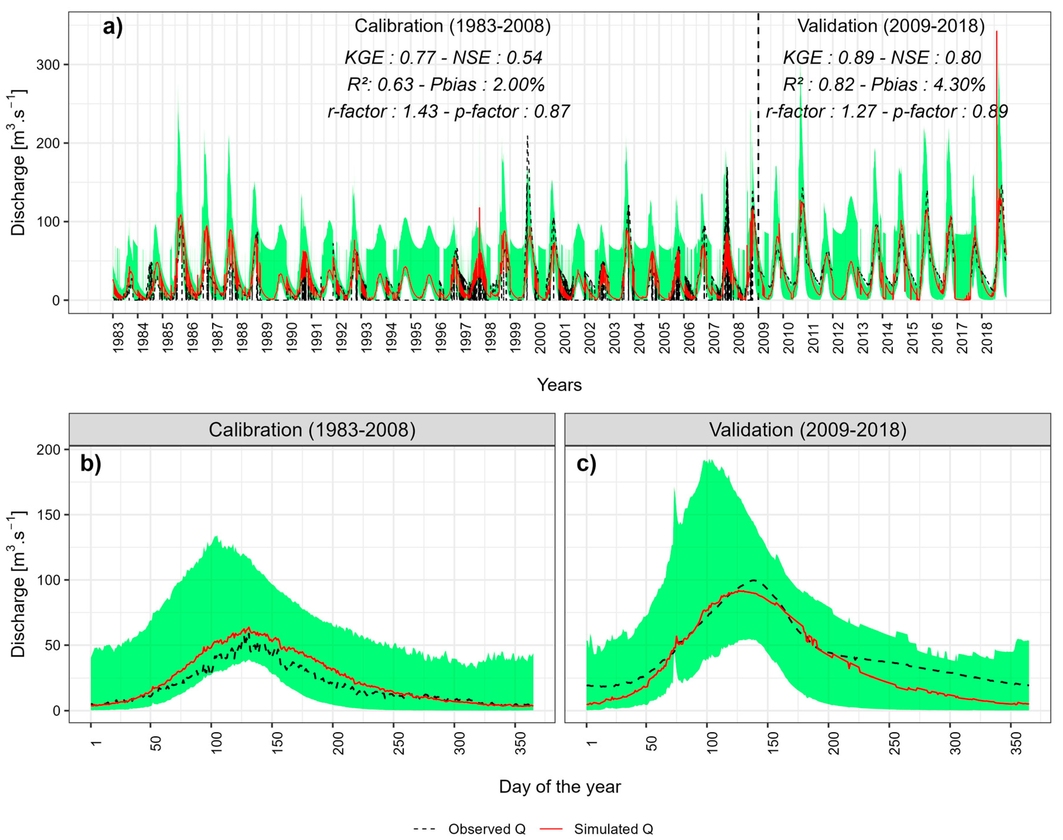
The model performance on both calibration and validation periods is evaluated according to performance metrics presented in Table 3. The calibrated model shows satisfactory performance in the period 1983–2008, which is further superior during the validation period, probably because this latter period is shorter. Nevertheless, it appears that the model is successful at simulating surface runoff in the MRC. The average value of the observed daily discharge is 31.94 ± 32.27 m3·s−1 (45.41 ± 29.78 m3·s−1), while the simulated value average is 32.59 ± 29.23 m3·s−1 (47.43 ± 28.59 m3·s−1), respectively, on the calibration and validation periods. It should also be noted that the r_factor and p_factor on both calibration and validation periods are optimal, meaning that the uncertainty 95PPU band around the simulated values is not significantly larger than the variability in observations and that a significant portion of those observations are captured within this envelope [52,55].
Figure 5 shows the time series of daily simulations over the study period 1983–2018, which further highlights the model performance at reproducing observed patterns in streamflow.
Figure 6 shows the Flow Duration Curve (FDC) for simulated and observed daily discharges, over the period 1983–2018, which shows that the model overall reproduces well the quantile distribution of daily values. However, it could be further noted that the high flows (having the lowest exceedance probabilities, <40%) are overestimated, while low flows (having the highest exceedance probabilities, >60%) are underestimated.
3.3. Hydrological Balance of the MRC
Table 4 shows the average annual values of the main hydrologic processes in the MRC as represented by the calibrated SWAT model. The average annual rainfall and PET are 952.1 ± 130.4 mm and 1940.4 ± 51.1 mm (respectively), of which 199.1 ± 72.2 mm are converted to surface runoff (i.e., a surface runoff coefficient of 20.91%). The actual evapotranspiration ET is estimated at 459.6 ± 33.6 mm on an annual average (i.e., 48.27% of the annual rainfall). Also, the average annual groundwater recharge (DEEPAQ) reaches 23.3 ± 5.6 mm, i.e., 2.44% of the annual rainfall.
Figure 7 shows the spatial variation of average annual rainfall, actual evapotranspiration ET, and surface runoff within the catchment. An increasing rainfall gradient (north to south) is observed (Figure 7a). ET follows the same gradient (Figure 7b), indicating that ET is mostly conditioned by available water excess in different sub-catchments in the MRC. The highest annual surface runoff amounts (Figure 7c) are generated in the north-western sub-catchments followed by the southernmost sub-catchments, where soil surface conditions are mostly barren or degraded and less natural vegetation is found, indicating that the rainfall–runoff generation is sensitive to soil surface conditions in the MRC.
3.4. Effects of Climate Variability on Surface Runoff
3.4.1. Correlation and Trends
The Spearman rank correlation analysis reveals that at the annual scale, rainfall is significantly and positively correlated with surface runoff (ρ = 0.732, p-value < 0.0001). On the other hand, PET shows a negative association with surface runoff, although not statistically significant (ρ = −0.148, p-value = 0.386). This could further be explained by the fact that evapotranspiration is a latent hydrological process, mostly active during dry periods between successive rainfall events, while rainfall is the major process providing entering flux in the hydrological system and responsible for the onset of surface runoff.
The trends in annual rainfall, ET, and surface runoff are presented in Figure 8.
The trend in annual rainfall in the MRC is significant (p-value = 0.029), with an increase of 4.98 mm·year−1 over the period 1983–2018. Annual PET, however, appears to be stationary (p-value = 0.307, not significant), with a slope of increase of about 1.55 mm·year−1. Annual surface runoff shows a significant increasing trend of 0.45 m3 s−1·year−1 (p-value = 0.013), largely caused by the trend observed in rainfall over the study period.
Figure 9 further highlights the patterns of increase in surface runoff over successive decades, from the 1980s to 2010s on both monthly averages (Figure 9a) and flow duration curves (Figure 9b). A decrease is observed from the 1980s to the 1990s, then an increase in average monthly surface runoff and high-to-median quantiles is observed from the 1990s onwards. This also highlights implications for the sizing of future hydraulic infrastructures, especially check dams [8].
3.4.2. Elasticity of P, PET, and Environmental Conditions in the MRC
Figure 10 shows the elasticities of P, PET, and environmental conditions to surface runoff in the MRC.
The analysis shows that surface runoff is highly sensitive to rainfall (R² = 0.54), as given by the elastic coefficient of 2.002, suggesting that an increase of 1% in the annual rainfall results in an increase of 2% in annual surface runoff. Also, surface runoff is less sensitive to PET, with an elasticity of −1.804, suggesting that an increase in annual PET results in drier catchment conditions, causing a decrease in annual surface runoff. Finally, surface runoff is also less sensitive to environmental conditions, with an elasticity of 0.270, which outlines that the catchment evolution tends towards an increase in annual surface runoff. Also, it should be noted that the sensitivities of surface runoff to PET and environmental conditions are not significant (R² = 0.022 and 0.012, respectively).
3.4.3. Modes of Variability in P, PET, and Surface Runoff
Figure 11 shows the modes of variability in rainfall, PET and surface runoff, as depicted by wavelet power spectra shown in Figure 10d–f. The annual rainfall wavelet power spectrum shows high and significant fluctuations in 2007–2012 in the 2–4-year band (Figure 10d). The annual PET wavelet power spectrum shows a hint of significant fluctuations in 1997–1998 and in 2010 in the 2–4-year band and strong quasi-decadal significant fluctuation in 1997–2008 in the 4–8-year band (Figure 10e). The annual surface runoff wavelet power spectrum shows only significant fluctuations in 2010–2012 in the 2–4-year band (Figure 10f), which appears to be related to rainfall fluctuations at the same timescale, although being further modulated by external factors, probably catchment properties [14,73].
Figure 12 further investigates the multiscale phase–antiphase relationship between rainfall and surface runoff and between PET and surface runoff through the analysis of wavelet coherence transform (WCT). The arrows indicate the phase relationship between the two variables: arrows point to the right (left) when the time series are in phase (anti-phase) or when they are positively (negatively) correlated. Also, arrows pointing up mean that the first variable leads the second by 90°, whereas arrows pointing down indicate that the second variable leads the first by 90° [5,73,74]. In Figure 11a, continuously over the 1983–2018 period in the 2–16-year band, the phase relationship reveals that rainfall is the primary driver of surface runoff at all timescales, with the two series being in phase (highly correlated). In Figure 11b, it appears that PET is significantly in phase from 2003–2012 with surface runoff, however, being led by 90° in the 2–4-year band. Also, a significant quasi-decadal zero-phase from 1993–2007 is observed, indicating that the two variables move together over this sub-period.
4. Discussion and Conclusions
This study analyzed the impact of climate variability on hydrological processes in the MRC in Burkina Faso, in the West African Sahel, with a focus on surface runoff response. Hydrological modeling is used to reconstitute complete and gap-free records of surface runoff and further analyze the various components of the hydrological balance over the period 1983–2018. Overall, it appears that rainfall is the dominant driver of surface runoff, further modulated to a lesser extent by potential evapotranspiration at a quasi-decadal timescale. Also, the findings suggest that catchment properties may also play a role in the variability of surface runoff in the MRC, considering that a significant proportion of variability in surface runoff remains unexplained by rainfall and PET, and that the evolution in environmental changes tends towards a higher surface runoff potential generation. However, the study did not address the quantification of the isolated contribution of these sources of variation.
The West African Sahel in general is already acknowledged in the literature as one of the regions marked by extreme climate variability, which has profound implications for the regional hydrology [13,18,73,79]. This further explains why populations in the region are particularly vulnerable to climate stress since the water availability is mostly driven by rainfall. Recent climate changes, including erratic rainfall patterns and temperature increases, have created significant challenges for the region’s hydrological response. Yet, the hydrology in the region, in terms of quantification, understanding of the processes operating at various timescales and interactions between such processes, and direct and indirect implications on the availability of water resources remain understudied [12]. This further creates severe impediments to the development of well-informed, adapted, and resilient water management policies.
The integration of hydrological modeling, as carried out in this study, coupled with the use of global gridded datasets can help alleviate the knowledge gap [14,31]. These models help researchers and policymakers understand how changes in precipitation and temperature affect water resources and runoff patterns but also soil erosion [80]. In this study, it was shown that the MRC at Nowkuy gauging station is characterized by a significant upward trend in cumulative rainfall and potential evapotranspiration (to a lesser extent), which is further propagated to surface runoff showing an increase over the period 1983–2018. These findings are in line with previous observations [10,11,14,15,81,82,83], which also highlighted the important role of climate in surface runoff generation, especially in West African environments. In this regard, it should be outlined that the use of the MERRA-2 reanalysis data helped in representing spatial patterns in the rainfall over the catchment, which was certainly critical in attaining optimal model calibration. Therefore, the potential of using reanalysis datasets in hydrological modeling should be further explored as a potential and viable pathway to improve hydrological modeling efforts in data-scarce, poorly gauged, or even ungauged catchments, which are quite common in the West African Sahel [19,42].
Finally, since surface runoff response is acknowledged to be mainly driven by rainfall patterns in the MRC in this study, implications for future water availability should be explored through climate models. Previous studies analyzing the future projections of climate consistently highlight the increase in temperature and, therefore, potential evapotranspiration, but also changes in rainfall patterns, which are likely to result in a decrease in surface water availability [1,2,84]. This has been highlighted in local assessments in the region, especially with the recent launch of the CMIP6 global gridded climate projections [15]. However, in-depth and large-scale studies are essential to bridging the knowledge gap regarding the impacts of climate variability on surface runoff in Burkina Faso and the wider West African Sahel. This will further enable researchers and policymakers to better understand and anticipate the hydrological consequences of climate change, facilitating the development of targeted adaptation strategies to address water resource challenges and enhance resilience in the face of a globally changing climate.
Author Contributions
Conceptualization, C.O.Z., A.K. and R.Y.; methodology, A.K., R.Y. and B.M.; software, A.K., R.Y. and B.M.; validation, C.O.Z., A.K., R.Y. and B.M.; formal analysis, C.O.Z., A.K. and R.Y.; investigation, C.O.Z., A.K., R.Y. and B.M.; resources, A.K. and B.M.; data curation, A.K. and R.Y.; writing—original draft preparation, C.O.Z., A.K. and R.Y.; writing—review and editing, A.K., R.Y. and B.M.; visualization, A.K. and R.Y.; supervision, R.Y. All authors have read and agreed to the published version of the manuscript.
Funding
This research received no external funding.
Data Availability Statement
The code (under the R programming language) and the generated data supporting the results and the figures in this study are all publicly available on GitHub (https://github.com/kiema97/HydroModelNowkuy (accessed on 21 September 2023)). The daily climate observations at the synoptic stations of Bobo-Dioulasso and Dédougou in Burkina Faso can be obtained through a request to the National Meteorology Agency in Burkina Faso (ANAM-BF).
Acknowledgments
The authors are thankful to the National Meteorology Agency (ANAM-BF) for their support during this study.
Conflicts of Interest
The authors declare no conflict of interest.
References
- Stanzel, P.; Kling, H.; Bauer, H. Climate Change Impact on West African Rivers under an Ensemble of CORDEX Climate Projections. Clim. Serv. 2018, 11, 36–48. [Google Scholar] [CrossRef]
- Sylla, M.B.; Pal, J.S.; Faye, A.; Dimobe, K.; Kunstmann, H. Climate Change to Severely Impact West African Basin Scale Irrigation in 2 °C and 1.5 °C Global Warming Scenarios. Sci. Rep. 2018, 8, 14395. [Google Scholar] [CrossRef]
- Lèye, B.; Zouré, C.O.; Yonaba, R.; Karambiri, H. Water Resources in the Sahel and Adaptation of Agriculture to Climate Change: Burkina Faso. In Climate Change and Water Resources in Africa; Diop, S., Scheren, P., Niang, A., Eds.; Springer International Publishing: Cham, Switzerland, 2021; pp. 309–331. ISBN 978-3-030-61224-5. [Google Scholar]
- Bagré, P.M.; Yonaba, R.; Sirima, A.B.; Somé, Y.C.S. Influence Des Changements d’utilisation Des Terres Sur Les Débits Du Bassin Versant Du Massili à Gonsé (Burkina Faso). Vertigo 2023, 23, 39765. [Google Scholar] [CrossRef]
- Fowé, T.; Yonaba, R.; Mounirou, L.A.; Ouédraogo, E.; Ibrahim, B.; Niang, D.; Karambiri, H.; Yacouba, H. From Meteorological to Hydrological Drought: A Case Study Using Standardized Indices in the Nakanbe River Basin, Burkina Faso. Nat. Hazards 2023, 1–25. [Google Scholar] [CrossRef]
- Ibrahim, B. Characterization of the Rainy Seasons in Burkina Faso under a Climate Change Condition and Hydrological Impacts in the Nakanbé Basin. Ph.D. Thesis, Université Pierre et Marie Curie—Paris VI, Paris, France, 2012. [Google Scholar]
- Diedhiou, A.; Bichet, A.; Wartenburger, R.; Seneviratne, S.I.; Rowell, D.P.; Sylla, M.B.; Diallo, I.; Todzo, S.; Touré, N.E.; Camara, M.; et al. Changes in Climate Extremes over West and Central Africa at 1.5 °C and 2 °C Global Warming. Environ. Res. Lett. 2018, 13, 065020. [Google Scholar] [CrossRef]
- Fowé, T.; Diarra, A.; Kabore, R.F.W.; Ibrahim, B.; Bologo/Traoré, M.; Traoré, K.; Karambiri, H. Trends in Flood Events and Their Relationship to Extreme Rainfall in an Urban Area of Sahelian West Africa: The Case Study of Ouagadougou, Burkina Faso. J. Flood Risk Manag. 2019, 12, e12507. [Google Scholar] [CrossRef]
- Todzo, S.; Bichet, A.; Diedhiou, A. Intensification of the Hydrological Cycle Expected in West Africa over the 21st Century. Earth Syst. Dyn. 2020, 11, 319–328. [Google Scholar] [CrossRef]
- Amogu, O.; Descroix, L.; Yéro, K.S.; Le Breton, E.; Mamadou, I.; Ali, A.; Vischel, T.; Bader, J.-C.; Moussa, I.B.; Gautier, E.; et al. Increasing River Flows in the Sahel? Water 2010, 2, 170–199. [Google Scholar] [CrossRef]
- Amogu, O.; Esteves, M.; Vandervaere, J.-P.; Malam Abdou, M.; Panthou, G.; Rajot, J.-L.; Souley Yéro, K.; Boubkraoui, S.; Lapetite, J.-M.; Dessay, N.; et al. Runoff Evolution Due to Land-Use Change in a Small Sahelian Catchment. Hydrol. Sci. J. 2015, 60, 78–95. [Google Scholar] [CrossRef]
- Paturel, J.E.; Mahé, G.; Diello, P.; Barbier, B.; Dezetter, A.; Dieulin, C.; Karambiri, H.; Yacouba, H.; Maiga, A. Using Land Cover Changes and Demographic Data to Improve Hydrological Modeling in the Sahel: Improving Hydrological Modelling in the Sahel. Hydrol. Process. 2017, 31, 811–824. [Google Scholar] [CrossRef]
- Descroix, L.; Guichard, F.; Grippa, M.; Lambert, L.; Panthou, G.; Mahé, G.; Gal, L.; Dardel, C.; Quantin, G.; Kergoat, L.; et al. Evolution of Surface Hydrology in the Sahelo-Sudanian Strip: An Updated Review. Water 2018, 10, 748. [Google Scholar] [CrossRef]
- Yonaba, R.; Biaou, A.C.; Koïta, M.; Tazen, F.; Mounirou, L.A.; Zouré, C.O.; Queloz, P.; Karambiri, H.; Yacouba, H. A Dynamic Land Use/Land Cover Input Helps in Picturing the Sahelian Paradox: Assessing Variability and Attribution of Changes in Surface Runoff in a Sahelian Watershed. Sci. Total Environ. 2021, 757, 143792. [Google Scholar] [CrossRef]
- Yonaba, R.; Mounirou, L.A.; Tazen, F.; Koïta, M.; Biaou, A.C.; Zouré, C.O.; Queloz, P.; Karambiri, H.; Yacouba, H. Future Climate or Land Use? Attribution of Changes in Surface Runoff in a Typical Sahelian Landscape. Comptes Rendus Géosci. 2023, 355, 1–28. [Google Scholar] [CrossRef]
- Fox, P.; Rockström, J. Supplemental Irrigation for Dry-Spell Mitigation of Rainfed Agriculture in the Sahel. Agric. Water Manag. 2003, 61, 29–50. [Google Scholar] [CrossRef]
- Doto, C.V.; Yacouba, H.; Niang, D.; Lahmar, R.; Kossi Agbossou, E. Mitigation Effect of Dry Spells in Sahelian Rainfed Agriculture: Case Study of Supplemental Irrigation in Burkina Faso. Afr. J. Agric. Res. 2015, 10, 1863–1873. [Google Scholar] [CrossRef]
- Zougmoré, F.; Damiba, L.; D’Haen, S.; Dayamba, S.D. Projet d’Appui Scientifique Aux Processus de Plans Nationaux d’Adaptation (PAS-PNA)—État Des Lieux Des Connaissances Scientifiques Sur Les Ressources En Eau Au Burkina Faso et de l’impact Des Changements Climatiques Sur Ces Ressources (Scientific Support Project for National Adaptation Plan Processes—State of Scientific Knowledge on Water Resources in Burkina Faso and the Impact of Climate Change on These Resources); Climate Analytics gGmbH: Berlin, Germany, 2019. [Google Scholar]
- Dembélé, M.; Vrac, M.; Ceperley, N.; Zwart, S.J.; Larsen, J.; Dadson, S.J.; Mariéthoz, G.; Schaefli, B. Contrasting Changes in Hydrological Processes of the Volta River Basin under Global Warming. Hydrol. Earth Syst. Sci. 2022, 26, 1481–1506. [Google Scholar] [CrossRef]
- Nka, B.N.; Oudin, L.; Karambiri, H.; Paturel, J.E.; Ribstein, P. Trends in Floods in West Africa: Analysis Based on 11 Catchments in the Region. Hydrol. Earth Syst. Sci. 2015, 19, 4707–4719. [Google Scholar] [CrossRef]
- Tirogo, J.; Jost, A.; Biaou, A.; Valdes-Lao, D.; Koussoubé, Y.; Ribstein, P. Climate Variability and Groundwater Response: A Case Study in Burkina Faso (West Africa). Water 2016, 8, 171. [Google Scholar] [CrossRef]
- Kouanda, B.; Coulibaly, P.; Niang, D.; Fowe, T.; Karambiri, H.; Paturel, J.E. Analysis of the Performance of Base Flow Separation Methods Using Chemistry and Statistics in Sudano-Sahelian Watershed, Burkina Faso. Hydrol. Curr. Res. 2018, 9, 1000300. [Google Scholar] [CrossRef]
- Belemtougri, A.P.; Ducharne, A.; Tazen, F.; Oudin, L.; Karambiri, H. Understanding Key Factors Controlling the Duration of River Flow Intermittency: Case of Burkina Faso in West Africa. J. Hydrol. Reg. Stud. 2021, 37, 100908. [Google Scholar] [CrossRef]
- Tirogo, J.; Jost, A.; Biaou, A.; Koussoubé, Y.; Ribstein, P.; Dakouré, D. Impacts of Climate Change and Pumping on Groundwater Resources in the Kou River Basin, Burkina Faso. Comptes Rendus Géosci. 2023, 355, 1–25. [Google Scholar] [CrossRef]
- Yonaba, R.; Tazen, F.; Cissé, M.; Mounirou, L.A.; Belemtougri, A.; Ouedraogo, V.A.; Koïta, M.; Niang, D.; Karambiri, H.; Yacouba, H. Trends, Sensitivity and Estimation of Daily Reference Evapotranspiration ET0 Using Limited Climate Data: Regional Focus on Burkina Faso in the West African Sahel. Theor. Appl. Clim. 2023, 153, 947–974. [Google Scholar] [CrossRef]
- Arnold, J.; Srinivasan, R.; Muttiah, R.S.; Williams, J.R. Large Area Hydrologic Modeling and Assessment Part I: Model Development. J. Am. Water Resour. Assoc. 1998, 34, 73–89. [Google Scholar] [CrossRef]
- Neitsch, S.; Arnold, J.; Kiniry, J.R.; Williams, J.R. Soil and Water Assessment Tool Theoretical Documentation: Version 2009; Texas Water Resources Institute: College Station, TX, USA, 2011. [Google Scholar]
- Angelina, A.; Gado Djibo, A.; Seidou, O.; Seidou Sanda, I.; Sittichok, K. Changes to Flow Regime on the Niger River at Koulikoro under a Changing Climate. Hydrol. Sci. J. 2015, 60, 1709–1723. [Google Scholar] [CrossRef]
- Chaibou Begou, J.; Jomaa, S.; Benabdallah, S.; Bazie, P.; Afouda, A.; Rode, M. Multi-Site Validation of the SWAT Model on the Bani Catchment: Model Performance and Predictive Uncertainty. Water 2016, 8, 178. [Google Scholar] [CrossRef]
- Yonaba, R. Spatiotemporal Land Use and Land Cover Dynamics and Impact on Surface Runoff in a Sahelian Landscape: Case of Tougou Watershed (Northern Burkina Faso). Ph.D. Thesis, International Institute for Water and Environmental Engineering (2iE), Ouagadougou, Burkina Faso, 2020. [Google Scholar]
- Gbohoui, Y.P.; Paturel, J.-E.; Fowe, T.; Mounirou, L.A.; Yonaba, R.; Karambiri, H.; Yacouba, H. Impacts of Climate and Environmental Changes on Water Resources: A Multi-Scale Study Based on Nakanbé Nested Watersheds in West African Sahel. J. Hydrol. Reg. Stud. 2021, 35, 100828. [Google Scholar] [CrossRef]
- Hawker, L.; Neal, J. FABDEM V1-0 2021; University of Bristol: Bristol, UK, 2021. [Google Scholar]
- Bonzi, W.M.-E.; Vanderhaeghe, O.; Van Lichtervelde, M.; Wenmenga, U.; André-Mayer, A.-S.; Salvi, S.; Poujol, M. Petrogenetic Links between Rare Metal-Bearing Pegmatites and TTG Gneisses in the West African Craton: The Mangodara District of SW Burkina Faso. Precambrian Res. 2021, 364, 106359. [Google Scholar] [CrossRef]
- Kafando, M.B.; Koïta, M.; Le Coz, M.; Yonaba, O.R.; Fowe, T.; Zouré, C.O.; Faye, M.D.; Leye, B. Use of Multidisciplinary Approaches for Groundwater Recharge Mechanism Characterization in Basement Aquifers: Case of Sanon Experimental Catchment in Burkina Faso. Water 2021, 13, 3216. [Google Scholar] [CrossRef]
- Kafando, M.B.; Koïta, M.; Zouré, C.O.; Yonaba, R.; Niang, D. Quantification of Soil Deep Drainage and Aquifer Recharge Dynamics According to Land Use and Land Cover in the Basement Zone of Burkina Faso in West Africa. Sustainability 2022, 14, 14687. [Google Scholar] [CrossRef]
- IGB. Base de Données d’Occupation Des Terres (BDOT) 2012, Burkina Faso; IGNFI: Paris, France, 2012. [Google Scholar]
- FAO; IIASA; ISRIC; ISSCAS; JRC. Harmonized World Soil Database (Version 1.2); Food and Agriculture Organization: Rome, Italy; International Institute for Applied Systems Analysis: Laxenburg, Austria, 2012. [Google Scholar]
- Gelaro, R.; McCarty, W.; Suárez, M.J.; Todling, R.; Molod, A.; Takacs, L.; Randles, C.A.; Darmenov, A.; Bosilovich, M.G.; Reichle, R.; et al. The Modern-Era Retrospective Analysis for Research and Applications, Version 2 (MERRA-2). J. Clim. 2017, 30, 5419–5454. [Google Scholar] [CrossRef]
- Sparks, A.H. Ropensci/Nasapower, V4.0.9; 2023. Available online: https://cran.r-project.org/web/packages/nasapower/index.html (accessed on 10 September 2023).
- Hawker, L.; Uhe, P.; Paulo, L.; Sosa, J.; Savage, J.; Sampson, C.; Neal, J. A 30 m Global Map of Elevation with Forests and Buildings Removed. Environ. Res. Lett. 2022, 17, 024016. [Google Scholar] [CrossRef]
- Dembélé, M.; Zwart, S.J. Evaluation and Comparison of Satellite-Based Rainfall Products in Burkina Faso, West Africa. Int. J. Remote Sens. 2016, 37, 3995–4014. [Google Scholar] [CrossRef]
- Dembélé, M.; Schaefli, B.; van de Giesen, N.; Mariéthoz, G. Suitability of 17 Gridded Rainfall and Temperature Datasets for Large-Scale Hydrological Modelling in West Africa. Hydrol. Earth Syst. Sci. 2020, 24, 5379–5406. [Google Scholar] [CrossRef]
- Michelangeli, P.-A.; Vrac, M.; Loukos, H. Probabilistic Downscaling Approaches: Application to Wind Cumulative Distribution Functions. Geophys. Res. Lett. 2009, 36, L11708. [Google Scholar] [CrossRef]
- Vrac, M.; Drobinski, P.; Merlo, A.; Herrmann, M.; Lavaysse, C.; Li, L.; Somot, S. Dynamical and Statistical Downscaling of the French Mediterranean Climate: Uncertainty Assessment. Nat. Hazards Earth Syst. Sci. 2012, 12, 2769–2784. [Google Scholar] [CrossRef]
- Vrac, M.; Michelangeli, P.-A. CDFt: Downscaling and Bias Correction via Non-Parametric CDF-Transform. 2021. Available online: https://rdrr.io/cran/CDFt/ (accessed on 10 September 2023).
- Hargreaves, G.H.; Samani, Z.A. Reference Crop Evapotranspiration from Temperature. Appl. Eng. Agric. 1985, 1, 96–99. [Google Scholar] [CrossRef]
- Raziei, T.; Pereira, L.S. Estimation of ETo with Hargreaves–Samani and FAO-PM Temperature Methods for a Wide Range of Climates in Iran. Agric. Water Manag. 2013, 121, 1–18. [Google Scholar] [CrossRef]
- Zouré, C.; Queloz, P.; Koïta, M.; Niang, D.; Fowé, T.; Yonaba, R.; Consuegra, D.; Yacouba, H.; Karambiri, H. Modelling the Water Balance on Farming Practices at Plot Scale: Case Study of Tougou Watershed in Northern Burkina Faso. Catena 2019, 173, 59–70. [Google Scholar] [CrossRef]
- Mockus, V. Estimation of Direct Runoff from Storm Rainfall. In Part 630 Hydrology; National Engineering Handbook; USDA: Washington, DC, USA, 1972; Volume 4. [Google Scholar]
- Williams, J.R. Flood Routing with Variable Travel Time or Variable Storage Coefficients. Trans. ASAE 1969, 12, 100–103. [Google Scholar] [CrossRef]
- Sood, A.; Muthuwatta, L.; McCartney, M. A SWAT Evaluation of the Effect of Climate Change on the Hydrology of the Volta River Basin. Water Int. 2013, 38, 297–311. [Google Scholar] [CrossRef]
- Abbaspour, K.C.; Vejdani, M.; Haghighat, S.; Yang, J. SWAT-CUP Calibration and Uncertainty Programs for SWAT. In Proceedings of the MODSIM 2007 International Congress on Modelling and Simulation, Modelling and Simulation Society of Australia and New Zealand, Christchurch, New Zealand, 10–13 December 2007; pp. 1596–1602. [Google Scholar]
- Kling, H.; Fuchs, M.; Paulin, M. Runoff Conditions in the Upper Danube Basin under an Ensemble of Climate Change Scenarios. J. Hydrol. 2012, 424–425, 264–277. [Google Scholar] [CrossRef]
- Knoben, W.J.M.; Freer, J.E.; Woods, R.A. Technical Note: Inherent Benchmark or Not? Comparing Nash–Sutcliffe and Kling–Gupta Efficiency Scores. Hydrol. Earth Syst. Sci. 2019, 23, 4323–4331. [Google Scholar] [CrossRef]
- Abbaspour, K.C.; Johnson, C.A.; van Genuchten, M.T. Estimating Uncertain Flow and Transport Parameters Using a Sequential Uncertainty Fitting Procedure. Vadose Zone J. 2004, 3, 1340–1352. [Google Scholar] [CrossRef]
- Abbaspour, K.C.; Rouholahnejad, E.; Vaghefi, S.; Srinivasan, R.; Yang, H.; Kløve, B. A Continental-Scale Hydrology and Water Quality Model for Europe: Calibration and Uncertainty of a High-Resolution Large-Scale SWAT Model. J. Hydrol. 2015, 524, 733–752. [Google Scholar] [CrossRef]
- Moriasi, D.N.; Gitau, M.W.; Pai, N.; Daggupati, P. Hydrologic and Water Quality Models: Performance Measures and Evaluation Criteria. Trans. ASABE 2015, 58, 1763–1785. [Google Scholar] [CrossRef]
- Mann, H.B. Nonparametric Tests against Trend. Econometrica 1945, 13, 245. [Google Scholar] [CrossRef]
- Kendall, M.G. Multivariate Analysis; Griffin: London, UK, 1975; ISBN 978-0-85264-234-4. [Google Scholar]
- Yue, S.; Pilon, P.; Phinney, B.; Cavadias, G. The Influence of Autocorrelation on the Ability to Detect Trend in Hydrological Series. Hydrol. Process. 2002, 16, 1807–1829. [Google Scholar] [CrossRef]
- Patakamuri, S.K.; O’Brien, N. Modifiedmk: Modified Versions of Mann Kendall and Spearman’s Rho Trend Tests 2021. R Package Version 2020, 1. [Google Scholar]
- Sen, P.K. Estimates of the Regression Coefficient Based on Kendall’s Tau. J. Am. Stat. Assoc. 1968, 63, 1379–1389. [Google Scholar] [CrossRef]
- Theil, H. A Rank-Invariant Method of Linear and Polynomial Regression Analysis. In Henri Theil’s Contributions to Economics and Econometrics; Raj, B., Koerts, J., Eds.; Advanced Studies in Theoretical and Applied Econometrics; Springer: Dordrecht, The Netherlands, 1992; Volume 23, pp. 345–381. ISBN 978-94-010-5124-8. [Google Scholar]
- Spearman, C. The Proof and Measurement of Association between Two Things. Am. J. Psychol. 1904, 15, 72. [Google Scholar] [CrossRef]
- Schaake, J.C. From Climate to Flow. In Climate Change and US Water Resources.; Waggoner, P.E., Ed.; Wiley Series in Climate and the Biosphere; Wiley: Hoboken, NJ, USA, 1990; pp. 177–206. ISBN 978-0-471-61838-6. [Google Scholar]
- Ma, Y.; Sun, D.; Niu, Z.; Wang, X. Contribution of Climate Change and Human Activities to Runoff and Sediment Discharge Changes Based on Budyko Theory and Water–Sediment Relationships during 1960–2019 in the Taohe River Basin, China. Atmosphere 2023, 14, 1144. [Google Scholar] [CrossRef]
- Mo, C.; Lai, S.; Yang, Q.; Huang, K.; Lei, X.; Yang, L.; Yan, Z.; Jiang, C. A Comprehensive Assessment of Runoff Dynamics in Response to Climate Change and Human Activities in a Typical Karst Watershed, Southwest China. J. Environ. Manag. 2023, 332, 117380. [Google Scholar] [CrossRef] [PubMed]
- Mezentsev, V. More on the Calculation of Average Total Evaporation. Meteorol. Gidrol. 1955, 5, 24. [Google Scholar]
- Choudhury, B. Evaluation of an Empirical Equation for Annual Evaporation Using Field Observations and Results from a Biophysical Model. J. Hydrol. 1999, 216, 99–110. [Google Scholar] [CrossRef]
- Yang, H.; Yang, D.; Lei, Z.; Sun, F. New Analytical Derivation of the Mean Annual Water-energy Balance Equation. Water Resour. Res. 2008, 44, 2007WR006135. [Google Scholar] [CrossRef]
- Grinsted, A.; Moore, J.C.; Jevrejeva, S. Application of the Cross Wavelet Transform and Wavelet Coherence to Geophysical Time Series. Nonlinear Process. Geophys. 2004, 11, 561–566. [Google Scholar] [CrossRef]
- Torrence, C.; Compo, G.P. A Practical Guide to Wavelet Analysis. Bull. Amer. Meteor. Soc. 1998, 79, 61–78. [Google Scholar] [CrossRef]
- Sidibe, M.; Dieppois, B.; Eden, J.; Mahé, G.; Paturel, J.-E.; Amoussou, E.; Anifowose, B.; Lawler, D. Interannual to Multi-Decadal Streamflow Variability in West and Central Africa: Interactions with Catchment Properties and Large-Scale Climate Variability. Glob. Planet. Change 2019, 177, 141–156. [Google Scholar] [CrossRef]
- Gouhier, T.C.; Grinsted, A.; Simko, V. Biwavelet: Conduct Univariate and Bivariate Wavelet Analyses. 2019. Available online: https://rdrr.io/rforge/biwavelet/ (accessed on 10 September 2023).
- Stephens, G.L.; L’Ecuyer, T.; Forbes, R.; Gettelmen, A.; Golaz, J.-C.; Bodas-Salcedo, A.; Suzuki, K.; Gabriel, P.; Haynes, J. Dreary State of Precipitation in Global Models: Model and Observed Precipitation. J. Geophys. Res. 2010, 115. [Google Scholar] [CrossRef]
- Mounirou, L.A.; Zouré, C.O.; Yonaba, R.; Paturel, J.-E.; Mahé, G.; Niang, D.; Yacouba, H.; Karambiri, H. Multi-Scale Analysis of Runoff from a Statistical Perspective in a Small Sahelian Catchment under Semi-Arid Climate. Arab. J. Geosci. 2020, 13, 154. [Google Scholar] [CrossRef]
- Mounirou, L.A.; Yonaba, R.; Koïta, M.; Paturel, J.-E.; Mahé, G.; Yacouba, H.; Karambiri, H. Hydrologic Similarity: Dimensionless Runoff Indices across Scales in a Semi-Arid Catchment. J. Arid Environ. 2021, 193, 104590. [Google Scholar] [CrossRef]
- Yonaba, R.; Koïta, M.; Mounirou, L.A.; Tazen, F.; Queloz, P.; Biaou, A.C.; Niang, D.; Zouré, C.; Karambiri, H.; Yacouba, H. Spatial and Transient Modelling of Land Use/Land Cover (LULC) Dynamics in a Sahelian Landscape under Semi-Arid Climate in Northern Burkina Faso. Land Use Policy 2021, 103, 105305. [Google Scholar] [CrossRef]
- Sidibe, M.; Dieppois, B.; Mahé, G.; Paturel, J.-E.; Amoussou, E.; Anifowose, B.; Lawler, D. Trend and Variability in a New, Reconstructed Streamflow Dataset for West and Central Africa, and Climatic Interactions, 1950–2005. J. Hydrol. 2018, 561, 478–493. [Google Scholar] [CrossRef]
- Mounirou, L.A.; Yonaba, R.; Tazen, F.; Ayele, G.T.; Yaseen, Z.M.; Karambiri, H.; Yacouba, H. Soil Erosion across Scales: Assessing Its Sources of Variation in Sahelian Landscapes under Semi-Arid Climate. Land 2022, 11, 2302. [Google Scholar] [CrossRef]
- Lebel, T.; Ali, A. Recent Trends in the Central and Western Sahel Rainfall Regime (1990–2007). J. Hydrol. 2009, 375, 52–64. [Google Scholar] [CrossRef]
- Gal, L.; Grippa, M.; Hiernaux, P.; Pons, L.; Kergoat, L. The Paradoxical Evolution of Runoff in the Pastoral Sahel: Analysis of the Hydrological Changes over the Agoufou Watershed (Mali) Using the KINEROS-2 Model. Hydrol. Earth Syst. Sci. 2017, 21, 4591–4613. [Google Scholar] [CrossRef]
- Panthou, G.; Lebel, T.; Vischel, T.; Quantin, G.; Sane, Y.; Ba, A.; Ndiaye, O.; Diongue-Niang, A.; Diopkane, M. Rainfall Intensification in Tropical Semi-Arid Regions: The Sahelian Case. Environ. Res. Lett. 2018, 13, 064013. [Google Scholar] [CrossRef]
- Roudier, P.; Ducharne, A.; Feyen, L. Climate Change Impacts on Runoff in West Africa: A Review. Hydrol. Earth Syst. Sci. 2014, 18, 2789–2801. [Google Scholar] [CrossRef]
Figure 1.
Location of the Mouhoun River Catchment (MRC) in Burkina Faso, West Africa. Elevation data are provided by FABDEM [32].
Figure 1.
Location of the Mouhoun River Catchment (MRC) in Burkina Faso, West Africa. Elevation data are provided by FABDEM [32].

Figure 2.
Physical characterization of the Mouhoun River Catchment (MRC). (a) Soil types. (b) Land use/land cover (LULC) types. (c) Slope classes, calculated from the FABDEM dataset [32] used in this study.
Figure 2.
Physical characterization of the Mouhoun River Catchment (MRC). (a) Soil types. (b) Land use/land cover (LULC) types. (c) Slope classes, calculated from the FABDEM dataset [32] used in this study.

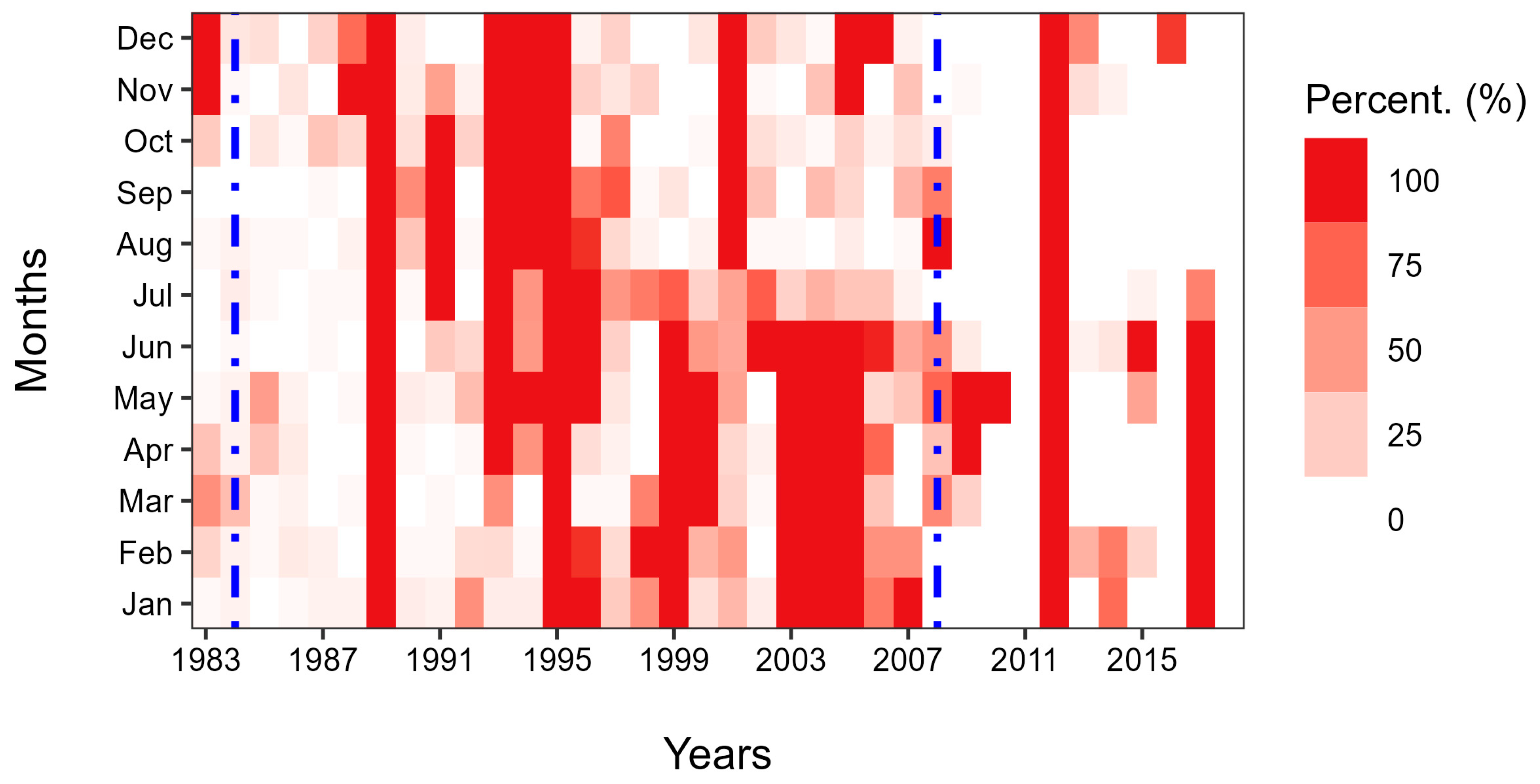
Figure 3.
Distribution of gaps in the observed dataset of daily discharge at Nowkuy gauging station. The years 1989, 1995, and 2012 are completely missing observed data. The dashed blue lines indicate the limits of the warm-up (1983–1984), calibration (1985–2008), and validation (2009–2018) periods.

Figure 4.
Empirical cumulative distribution functions showing bias-correction adjustment through the CDFt method for MERRA-2 reanalysis and observed data. The top panels are for the synoptic station of Bobo-Dioulasso, while the bottom panels are for the station of Dédougou. On each row, panels show, left to right, daily rainfall, maximum temperature (Tmax), and minimum temperature (Tmin) over the period 1983–2018.

Figure 5.
Observed and simulated discharge of the calibrated SWAT model in the MRC over the period 1983–2018. (a) Daily time series. (b) Daily average annual observed and simulated discharge over the calibration period. (c) Daily average annual observed and simulated discharge over the validation period. The green band shows the 95PPU envelope around simulated values.

Figure 6.
Observed and simulated flow duration curves (FDCs) in the MRC over the period 1983–2018.

Figure 7.
Spatial variation of average annual values for: (a) Rainfall; (b) ET; (c) Surface runoff in the Mouhoun River Catchment (MRC) over the period 1983–2018.
Figure 7.
Spatial variation of average annual values for: (a) Rainfall; (b) ET; (c) Surface runoff in the Mouhoun River Catchment (MRC) over the period 1983–2018.

Figure 8.
Annual trend analysis using the modified Mann–Kendall test (at 5% significance level) in the MRC. (a) Annual rainfall. (b) Annual PET. (c) Annual discharge.
Figure 8.
Annual trend analysis using the modified Mann–Kendall test (at 5% significance level) in the MRC. (a) Annual rainfall. (b) Annual PET. (c) Annual discharge.

Figure 9.
Decadal changes in surface runoff over the 1983–2018 period in the MRC. (a) Decadal changes in average monthly discharges. (b) Decadal changes in interannual Flow Duration Curves (FDCs).
Figure 9.
Decadal changes in surface runoff over the 1983–2018 period in the MRC. (a) Decadal changes in average monthly discharges. (b) Decadal changes in interannual Flow Duration Curves (FDCs).

Figure 10.
Elastic coefficients of rainfall (in (a)), PET (in (b)), and environmental conditions (in (c)) to surface runoff in the MRC over the period 1983–2018 in the MRC.
Figure 10.
Elastic coefficients of rainfall (in (a)), PET (in (b)), and environmental conditions (in (c)) to surface runoff in the MRC over the period 1983–2018 in the MRC.

Figure 11.
Modes of variability in rainfall, PET, and surface runoff over the period 1983–2018 in the MRC. (a–c) show the standardized values of rainfall, PET, and runoff, respectively. (d–f) show the continuous wavelet power spectra of rainfall, PET, and runoff, respectively. The thick black contour lines delimit the cone of influence (COI) outside which edge effects distort the signal and, therefore, are not considered in the analysis. Within the COI, significant fluctuations at a 10% level against red noise are outlined in thick black contour lines [14,72,73,74].

Figure 12.
Wavelet coherence over the period 1983–2018 in the MRC for (a) rainfall–surface runoff (P-Q) relationship and (b) PET–surface runoff (PET-Q) relationship. The thick black contour lines delimit the cone of influence (COI) outside which edge effects distort the signal and, therefore, are not considered in the analysis. Within the COI, significant fluctuations at a 10% level against red noise are outlined in thick black contour lines. Arrow line orientation indicates the phase relationship between the variables: pointing to the right indicates in-phase (0°) relationship, pointing to the left is out of phase (180°) relationship; pointing upward (downward) indicate that Q is led (Q is leading) by 90° the other variable.Overall, it appears that rainfall is the primary driver of surface runoff, at small to quasi-decadal timescales, and is leading surface runoff [76,77]. However, at quasi-decadal timescales, part of the variability in surface runoff is explained by PET. Finally, a significant portion of the variability in surface runoff remains unexplained by rainfall and PET, indicating that external factors, most likely changes in catchment properties (i.e., changes in LULC, [78]), are also affecting surface runoff generation mechanisms in the MRC.


Table 1.
SWAT Model parameters were selected for global sensitivity analysis in this study.
| Parameter Name | Description | Initial Range | Unit |
|---|---|---|---|
| Soil management, runoff generation parameters (1) | |||
| CN2 | SCS runoff curve number | 35–98 | - |
| Groundwater control parameters (10) | |||
| ALPHA_BF | Baseflow alpha factor | 0–1 | days−1 |
| GW_DELAY | Groundwater delay | 0–500 | days |
| SHALLST | Initial depth of water in the shallow aquifer | 0–50,000 | mm |
| DEEPST | Initial depth of water in the deep aquifer | 0–50,000 | mm |
| GWQMN | Depth of water (in the shallow aquifer) triggering return flow | 0–5000 | mm |
| GW_REVAP | Groundwater re-evaporation coefficient | 0.02–0.20 | - |
| REVAPMN | Water depth (in the shallow aquifer) triggering re-evaporation | 0–500 | mm |
| RCHRG_DP | Deep aquifer percolation fraction | 0–1 | - |
| GWHT | Initial groundwater height | 0–25 | m |
| GW_SPYLD | Specific yield of the shallow aquifer | 0.0–0.4 | m3 m−3 |
| Soil parameters (3) | |||
| SOL_Z | Depth from the soil surface to the bottom of the layer | 0–3500 | mm |
| SOL_AWC | Available water capacity of the soil layer | 0–1 | mm·m−1 |
| SOL_K | Saturated hydraulic conductivity | 0–2000 | mm h−1 |
| Channel and flow routing parameters (14) | |||
| CH_N2 | Manning’s roughness for the main channel | 0.01–0.3 | s·m−1/3 |
| CH_K2 | Effective hydraulic conductivity in main channel alluvium | 0.01–500 | mm·h−1 |
| ALPHA_BNK | Baseflow alpha factor for bank storage | 0–1 | days |
| CH_N1 | Manning’s roughness for tributary channels | 0.01–30 | s·m−1/3 |
| CH_K1 | Effective hydraulic conductivity in tributary channel alluvium | 0–300 | mm·h−1 |
| OV_N | Manning’s roughness for overland flow | 0.01–30 | s·m−1/3 |
| LAT_TTIME | Lateral flow travel time | 0–180 | days |
| CANMX | Maximum canopy storage | 0–100 | mm |
| ESCO | Soil evaporation compensation factor | 0–1 | - |
| EPCO | Plant uptake compensation factor | 0–1 | - |
| MSK_CO1 | Storage time constant for normal flow | 0–10 | - |
| MSK_CO2 | Storage time constant for low flow | 0–10 | - |
| MSK_X | Inflow/outflow rate in reach segment control weighting | 0–0.3 | - |
| TRNSRCH | Loss fraction from the main channel entering the deep aquifer | 0–1 | - |
Table 2.
Model parameters’ sensitivity ranking, fitted values, and uncertainty ranges.
| Sensitivity Rank | Parameter | Fitted Value | Uncertainty Range |
|---|---|---|---|
| 1 | r__CN2 | 0.265 | [0.101…0.464] |
| 2 | v__GW_DELAY | 56.649 | [0.000…112.623] |
| 3 | v__GWQMN | 1833.929 | [33.210…2110.164] |
| 4 | v__SHALLST | 14,511.832 | [13441.771…30983.770] |
| 5 | v__GW_REVAP | 0.195 | [0.143…0.196] |
| 6 | v__GWHT | 6.017 | [3.230…9.695] |
| 7 | v__GW_SPYLD | 0.117 | [0.087…0.195] |
| 8 | r__SOL_AWC | −0.841 | [−0.891…−0.293] |
| 9 | v__CH_N2 | 0.173 | [0.005…0.218] |
| 10 | v__CH_K2 | 374.704 | [289.448…452.462] |
| 11 | v__ALPHA_BNK | 0.799 | [0.509…0.846] |
| 12 | v__CH_K1 | 154.571 | [100.138…162.205] |
| 13 | v__EPCO | 0.359 | [0.036…0.372] |
| 14 | r__MSK_CO1 | −0.661 | [−0.690…−0.368] |
| 15 | v__TRNSRCH | 0.550 | [0.422…0.597] |
The prefix before each parameter name describes how the parameter is updated during the calibration process in SWAT-CUP: the relative mode (r__), in which the current value of the parameter is multiplied at each simulation by 1 + x, x being the given value; the value mode (v__), in which the current value of the parameter is replaced by a new value taken in a given interval. The uncertainty range around each parameter defines the uncertainty band (95PPU) around the simulated values [52]. The 15 parameters are ranked out in a decreasing order of global sensitivity, ranging from 1 (more sensitive) to 13 (less sensitive).
Table 3.
Model performance on calibration and validation periods.
| Performance Metric | Calibration (1983–2008) | Validation (2009–2018) |
|---|---|---|
| Observed/simulated mean Q (m3·s−1) | 31.94/32.59 | 45.41/47.43 |
| Observed/simulated standard deviation Q (m3·s−1) | 32.27/29.23 | 29.78/28.59 |
| KGE (objective function) | 0.77 | 0.89 |
| R² | 0.63 | 0.82 |
| NSE | 0.54 | 0.80 |
| PBIAS | 2.00% | 4.30% |
| r_factor | 1.43 | 1.27 |
| p_factor | 0.83 | 0.89 |
Table 4.
Average annual values of the hydrological processes simulated in the MRC over the period 1983–2018.
Table 4.
Average annual values of the hydrological processes simulated in the MRC over the period 1983–2018.
| Hydrological Process | Average Annual Values (±Standard Deviation) |
|---|---|
| Annual rainfall (P, mm) | 952.1 (±130.4) |
| Potential evapotranspiration (PET, mm) | 1940.4 (±51.1) |
| Actual evapotranspiration (ET, mm) | 459.6 (±33.6) |
| Surface runoff (Q, mm) | 199.1 (±72.2) |
| Soil water content (SW, mm) | 5.2 (±1.0) |
| Lateral flow (LATQ, mm) | 0.9 (±0.1) |
| Deep aquifer recharge (DEEPAQ, mm) | 23.3 (±5.6) |
Disclaimer/Publisher’s Note: The statements, opinions and data contained in all publications are solely those of the individual author(s) and contributor(s) and not of MDPI and/or the editor(s). MDPI and/or the editor(s) disclaim responsibility for any injury to people or property resulting from any ideas, methods, instructions or products referred to in the content. |
© 2023 by the authors. Licensee MDPI, Basel, Switzerland. This article is an open access article distributed under the terms and conditions of the Creative Commons Attribution (CC BY) license (https://creativecommons.org/licenses/by/4.0/).
Share and Cite
MDPI and ACS Style
Zouré, C.O.; Kiema, A.; Yonaba, R.; Minoungou, B. Unravelling the Impacts of Climate Variability on Surface Runoff in the Mouhoun River Catchment (West Africa). Land 2023, 12, 2017. https://0-doi-org.brum.beds.ac.uk/10.3390/land12112017
AMA Style
Zouré CO, Kiema A, Yonaba R, Minoungou B. Unravelling the Impacts of Climate Variability on Surface Runoff in the Mouhoun River Catchment (West Africa). Land. 2023; 12(11):2017. https://0-doi-org.brum.beds.ac.uk/10.3390/land12112017
Chicago/Turabian StyleZouré, Cheick Oumar, Arsène Kiema, Roland Yonaba, and Bernard Minoungou. 2023. "Unravelling the Impacts of Climate Variability on Surface Runoff in the Mouhoun River Catchment (West Africa)" Land 12, no. 11: 2017. https://0-doi-org.brum.beds.ac.uk/10.3390/land12112017
Note that from the first issue of 2016, this journal uses article numbers instead of page numbers. See further details here.