Article

Identifying Visual Quality of Rural Road Landscape Character by Using Public Preference and Heatmap Analysis in Sabak Bernam, Malaysia

1
Department of Landscape Architecture, Faculty of Design and Architecture, Universiti Putra Malaysia, Serdang 43400, Malaysia
2
Kulliyyah of Architecture and Environmental Design, International Islamic University Malaysia, Kuala Lumpur 53100, Malaysia
*
Authors to whom correspondence should be addressed.
Submission received: 28 June 2023 / Revised: 14 July 2023 / Accepted: 18 July 2023 / Published: 19 July 2023
(This article belongs to the Special Issue Landscape Architecture and Design in Urban and Peri-Urban Environment)

Abstract

:
The rural road landscape is crucial in forming rural areas’ landscape character (LC). As a platform for portraying the rural landscape, the rural roads demonstrate the area’s unique natural and cultural characteristics to visitors. However, with the continuous development of rural areas, the rural LC has been severely impacted, thus impacting visitors’ visual experience. In order to preserve and protect the rural landscape, this study aims to assess the visual quality of rural road landscapes based on public preference and heatmap analysis. The results indicated that most of the participants had a higher level of preference for rural landscapes with open horizontal views represented by agricultural areas, such as paddy fields. It was also found that different paddy field characters based on their planting stages can also positively affect the visual quality of rural road landscapes. The study also revealed that rural LCs with roadside settlements, commercial structures, mixed agricultural crops, and vegetation received low preference ratings. These characters negatively impact the visual quality of the rural road landscape. These findings provide significant insight for planners and decision-makers regarding protecting and preserving the essential rural road landscapes for the rural tourism experience.

1. Introduction

Rural regions have very distinct landscape patterns due to the effect of the region’s natural beauty, the style and form of the local architecture, and local cultural aspects [1]. In other words, the rural landscape is a particular sort of landscape that uses the countryside as the focal point and is characterized by a unique landscape [2]. The rural roads’ landscape characteristics typically consist of various land cover types, landforms, land use, rural historical sites, and artistic features [3]. As an essential component of the rural road, the rural plays a crucial role in the scenic experience in the local tourism industry [4]. Rural roads not only serve as vital connectors between communities but also as potential tourist routes for rural life experiences, scenic landscapes tours, and other relevant tourist attractions [5]. To some extent, the rural road landscape could be considered a valuable resource that can be used to promote and enhance local tourism activities. It can provide visitors a quick, easy, safe, and scenic experience to explore the countryside. Studies have shown that the rural roads’ landscapes could provide travelers with a positive experience through rural scenery and local cultural engagement [6,7,8].
However, in recent decades, rapid development and urban sprawl have changed and threatened the landscape’s appearance in rural areas [9,10]. Although the modernization processes have improved the living quality and enhanced basic facilities in the rural environment, they have also altered the appearance of the rural landscape [11,12]. Primdahl et al. [13] have identified that these changes are perceived as a threat, a harmful development that could damage the richness and distinctiveness of the original landscape. Changes in nature and the original appearance of the landscape in rural areas, without reasonable control, may lead to a decrease in the visual quality of the rural landscape [1,14]. Meanwhile, the change of land in rural areas has accelerated the process of fragmentation of the rural landscape, further generating negative impacts on the characteristics and affecting visual comfort in rural areas [15,16]. These changes may also decrease rural population satisfaction and a reduction in the usefulness of the landscape [17]. Many countries also emphasize the significance of protecting cultural and natural landscapes in response to development pressure [18]. Because of the numerous environmental changes related to these pressures, the idea of LC has been expanded to embrace not just extraordinary landscapes but also typical daily landscapes [19]. Therefore, nowadays, it can be seen that the awareness in the preservation of the original form of the landscape has received more attention and become particularly important.

Literature Review

Landscape character (LC) is defined as “a distinct, recognizable, and consistent pattern of elements in the landscape that makes one landscape different from another, rather than better or worse” [20]. The physical elements of the scene vary from one another, and bringing them together in one distinctive scene is known as “character” [21]. Koç and Yılmaz [22] have highlighted that LC could be seen as a notion and a process of differentiation based on its diversity, organization, and layout, ultimately providing each area a distinct personality that distinguishes it from the surrounding landscape. Each LC area is made up of a unique set of variables that reflect the landscape’s overall characteristics. LC may be defined as the landscape’s overall expression, which is reflected in several features, such as natural, cultural, visual, or symbolic. The quantification of LC as an indicator could describe and identify the scene, further measuring human preferences using visual quality [23]. Nonetheless, nature and culture are the most fundamental in defining LC. For instance, Simensen et al. [24] pointed out that the natural and cultural character of the landscapes has been included as an essential factor within the landscape character assessment (LCA) framework. LCA is a collection of tools and processes used to classify and describe landscapes, as well as to comprehend and convert the evolution of their physical and cultural traits into the development of the related management or planning policy [25]. As a result, LCA lays the groundwork for several policies to balance the contradictions that arise when multiple sectors use landscape resources [26].
Landscapes’ visual quality is determined by how an observer values the elements of the surrounding environment through their perception, emotional and psychological processes [27]. The landscape’s visual quality is based on the perceptual interaction between visitors and the landscape; hence, it can be subjectively quantified [28,29]. In contrast, some studies consider the landscape’s visual quality as dependent on the intrinsic characteristics of the environment [30]. Therefore, the visual quality of a landscape could be seen as coming from two primary sources: one is the elements and combinations of the landscape itself, while the other is the observer’s perception and perception of the landscape [14]. The first approach evaluates both the intensity of the characteristics and the objective and inherent beauty of the landscape itself [31,32]. These aspects can be evaluated quantitatively based on their physical or aesthetic components or other factors [33]. However, this approach ignores the observer’s subjective feelings, personal preferences, and psychological components, i.e., it leaves out the underlying hidden qualities of the landscape [34]. The second is a more intuitive way of assessing the landscape, using respondents’ preferences for the landscape, which means that each person needs to incorporate their understanding of the landscape into the assessment to reach a consensus [35]. Furthermore, certain authors have proposed a fusion of the two approaches [36,37], modifying the emphasis on integrating them based on practical considerations and aiming to establish a clearer relationship between landscape elements and the observer [38,39,40,41]. Therefore, landscape character and visual quality are essential to comprehending and assessing landscapes. However, their application requires careful consideration of the integration of objective and subjective assessments and the incorporation of different dimensions. Adopting a multidisciplinary approach encompassing diverse perspectives and disciplines can contribute to a more comprehensive and robust understanding of landscapes.
In Malaysia, rural-tourism-related projects have been progressing in recent years, with predominantly agricultural and agrarian tourism becoming popular, and the revenue from tourism gradually increasing [1]. However, along with development and other influences, the visual experience of Malaysia’s rural landscape has declined [42]. During this time, large portions of the rural population migrated to the city, resulting in a loss of cultural identity that may impact how the rural LC develops [13]. Hence, Malaysia’s rural visual experience and quality have become increasingly bleak. As mentioned earlier, the rural road is a significant component of rural areas and could indicate a place’s identity. It not only provides visitors with a taste of the local conditions or culture as they pass through but could also allow emotional attachment to the rural landscapes. Hence, the rural road landscapes’ visual quality has become a significant factor that can impact people’s experience. However, in Malaysia, only a few studies have focused on the visual aspect of rural road landscapes, leading to poor understanding among the decision-makers regarding its importance and future protection. Therefore, this study has three aims:
  • To classify and identify types of rural road LCs in Sabak Bernam in Malaysia;
  • To identify public preferences towards the visual quality based on rural road LCs in Sabak Bernam in Malaysia;
  • To identify preferred rural road landscape elements and socio-demographic factors that affect the preferences of rural road landscapes in Sabak Bernam, Malaysia.

2. Materials and Methods
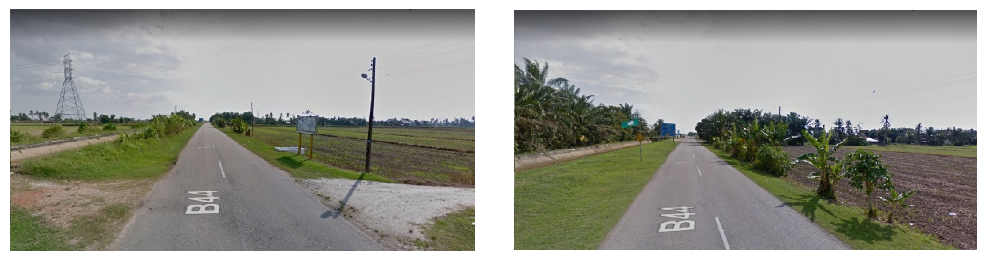
2.1. Study Area

The proposed study area is located within the Sabak Bernam district on the Malaysian Peninsula’s west coast. It borders Lower Perak District, Perak, to the north, the District of Kuala Selangor to the south, and the upper Hulu District to the east. It takes approximately 2 h of travel from Kuala Lumpur, the capital of Malaysia, to the study area. The majority of the district land areas are occupied by agriculture (47%) and forestry (40.18%), with less than 5% of the land being settlements and known as one of Malaysia’s major rice producer areas. Ibrahim et al. [43] mention that the road from Kuala Selangor to Sabak Bernam in the Malaysian government’s planning could be an attractive tourism route demonstrating the local rural landscape, such as culture, heritage, paddy fields, rural settlements, and tourist attractions. In addition to this, the related tourist services are relatively well equipped within the area. However, due to the conversion of paddy fields into commodity crops, housing, commercial and industrial, the acreage of paddy fields in Sabak Bernam has decreased over the past ten years, dropping from 26,645 hectares in 2000 to 13,375 hectares in 2013. Fortunately, due to food security and supply concerns, the government has recently started adopting measures and policies to protect the paddy field areas.
As one of the small towns in the district of Sabak Bernam, Sungai Besar, an area that retains its charms of rural character with traditional Malay architecture of “kampung houses”, vast areas of paddy fields and coconut plantations [44]. Sungai Besar is also well renowned for its homestay programs, which continue to preserve the rural way of life for tourists to enjoy. This study was specifically conducted on the rural road in Sungai Besar, starting from the junction of Jalan Sungai Panjang and Jalan Parit Cabang until the junction of Jalan Sungai Panjang and the rural path near Maktab Rendah Sains Mara Sungai Besar (Figure 1). This rural road is approximately 18.0 km (11.18 mi) long and is rich in scenic views of the rural landscape on both sides of the road.

2.2. Methods of the Study

Studies examining visual aesthetics have asserted that public preference for a landscape is an interactive phenomenon that results from the interplay between the physical attributes of the landscape and the psychological responses of individuals who observe it [45,46]. This study proposes a user-centered evaluation method based on a public understanding of landscape preferences using the Likert scale technique. The Likert scale, widely employed in educational and social science research, is one of the most basic and extensively utilized instruments in psychological measurement [47]. In general, using the Likert scale often balances both positive and negative items, aiming to mitigate bias in the response set [48]. The participants utilize a bipolar scale, consisting of options such as, “strongly disagree, disagree, neutral, agree, strongly agree”, to express their sentiments towards each item.
Furthermore, the photo survey method is one of the most direct approaches to assessing visual quality in the rural landscape [14]. The photo survey visually shows the scenic beauty of the landscape and allows the observer to assess its aesthetic appeal. Google Street View (https://www.google.com/maps, accessed on 1 February 2023) provided the photos for this investigation because it employs more comprehensive and high-resolution panoramic photographs and could be more effective, quicker, and more convenient than field-based techniques [49]. Besides, the heatmap analysis allows respondents to understand which LCs and elements are preferred. Today, heatmaps have gained popularity as a prevalent method of presenting information-rich data in 2D and 3D space. In terms of visualization, the graphical depiction of a heatmap provides a means of revealing coherent patterns within data by compressing a large amount of information into a small space [50]. Typically, two main categories of heatmaps exist the image-based heatmap and the data matrix heatmap [51]. The former refers to numerical data overlaid with an image, object, or geographic location, enabling visual information representation. The latter shows numerical information using a pseudo-color table or matrix format, presenting the information in a visual representation with specific color coding. Matrix heatmap finds extensive usage in the natural and biological sciences [52]. For this study, image-based heatmaps are an appropriate means of demonstrating data visualization and emphasizing the visual impact of specific landscape elements.

2.3. The First Phase

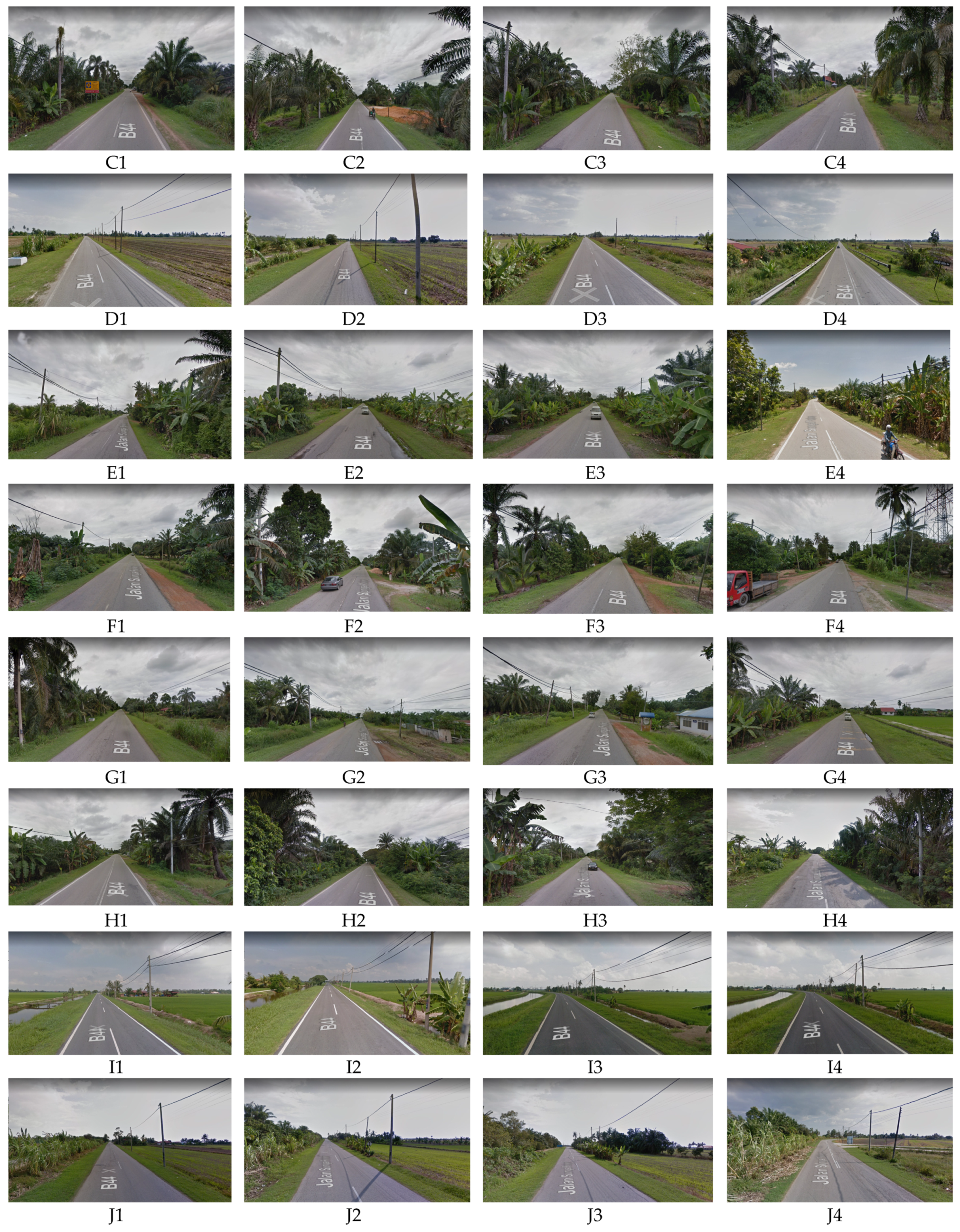
  • Collection of Photos
Photos along the rural road were captured through Google Street View at every 250 m interval to cover the selected rural road (approximately 18.0 km long, Figure 2). The interval was decided based on the rural roads’ 60 km/h speed restriction, equating to 60,000 m in 60 min. A vehicle traveling at this speed would cover a distance of 250 m in 15 s. The 15 s interval was chosen assuming that it would be a reasonable duration for a visitor to experience the totality of the landscape offered by driving through the rural road. Based on this approach, 72 photos were captured. The details of capturing and classifying photos were be explained in the next section.
  • Landscape Character Identification
This study classified the LCs in the collected photographs based on land use, landform, land cover, vegetation, and human-made structures. Twelve categories of LCs were eventually identified, each including at least four images of the same LC. There were 12 groups, from A to L, using upper case letters in sequential sequence as a code. Each group was labeled based on a particular LC, such as Group A: “Barren paddy fields with roadside vegetation”. To ensure that only dominant LC groups were selected for the survey, each group must have at least four photos. Based on this selection criteria, only 48 images were selected for this study after classification (Appendix A). Table 1 shows the code and label for each group with one photo.

2.4. The Second Phase

  • Survey
This study’s survey was administered and distributed online using a platform called Qualtrics. To avoid repetition of survey respondents’ responses, the images were randomly organized, and no images from the same group were allowed to be placed consecutively. Besides, two additional images were added (one at the beginning and another at the end) to allow respondents to familiarize themselves s with the survey procedures and to avoid having a misled result. However, results from these two additional images were excluded from the analysis.
This online preference survey has two sections: (A) the demographic and (B) the photo survey. Section (A) contains 11 general questions: age, gender, income, educational background, experience with rural road landscapes, and other questions that are also important to the study. Section (B) contains two parts. One is the use of a five-point Likert scale from 1 (least preferred) to 5 (highly preferred). Participants were asked to view and evaluate a rural road landscape scene in the photo. Each photo was given a visual quality score ranging from −2 (least preferred scene) to +2 (highly preferred scene), where 0 value means it is a moderate scene. Positive scores represent positive visual quality and vice versa. Using this categorization of the Likert scale, Wartmann et al. [53] successfully identified what the public considered an influential visual quality. Mundher et al. [54] successfully utilized this Likert scale to classify landscape characters into negative and positive visual quality categories. Another section is to allow respondents to click and identify two elements of photos that they like the most in the rural road landscape. Heatmap analysis will be automatically generated based on the recorded clicks’ intensity. The Qualtrics heatmap analysis was utilized to identify the LC that impacts the visual quality.
The final survey was distributed through social media using purposive sampling, limiting people living in Malaysia as participants. The survey data were collected over 30 days beginning 25 February 2023. The SPSS V26 program was used to analyze the survey results and identify the variables that influence visual quality evaluation. Figure 3 provides an overview of the research methodology employed in this study.

3. Results

3.1. Demographic Statistics Description

As shown in Table 2, 250 respondents out of 282 completed the survey, with more females (N = 155, 62%) than males (N = 95, 38%). A majority of the respondents (45.6%, N = 114) fell within the age group of 26 to 35 years old, while a significant portion (42%, N=105) belonged to the age group 18 to 25 years old. The remaining respondents (N = 31, 12.4%) were over 36 years old. Additionally, 108 respondents were foreigners, making up 43.2% of the total respondents, while 142 were Malaysians. Among Malaysians, the majority were Malays (N = 65, 26%) and Chinese (N = 67, 26.8%), while Indians were the minority (N = 10, 4%). On the other hand, among the international respondents, there were significantly more Chinese respondents (N = 97, 38.8%) than respondents from other nations (N = 11, 4.4%). More than half of the respondents were students (N = 131, 52.4%), which may indicate that their average monthly income was less than RM 2500 (N = 148, 48%). Moreover, over 80% of respondents (N = 222, 88%) in this group were educated higher than the high school level. Almost two-thirds of the (N = 160, 64%) respondents had a home in an urban area, while 35.2% (N = 88) reported visiting rural areas less than once a year. When the respondents were asked about the type of transportation they use when traveling to rural areas, the majority commented that the primary means of transport when traveling to rural areas was by car (N = 216, 86.4%). However, only a relatively small number of respondents stated that they have been to Sungai Besar. This accounted for 47 samples, representing 18.8% of the total respondents. Based on the results, it can be concluded that the respondents are predominantly female, students, and local; have a good education level; and are relatively familiar with rural areas but have limited information about the study area.
  • Statistics Description of Landscape Experience in Demographic Survey
This part depicted the extent to which respondents were intrigued by the experience of the rural environment (Table 3). In general, respondents exhibited a higher interest in the natural landscape (AM = 3.75) compared to cultural ones (AM = 3.288), particularly demonstrating the highest interest in the hills and mountains (IM = 3.83) in the natural landscape. However, traditional houses (IM = 3.67) and orchards (IM = 3.56) had a much higher average individual value in the cultural group than other LCs. Interestingly, the individual mean value for traditional houses (IM = 3.67) in the cultural LC variable was even higher than the forests (IM = 3.63) in the natural landscape variable. This result suggested that traditional rural houses could be of interest to some respondents because of their specific memories of their hometowns and their preference for traditional heritage. Paddy fields, mixed agricultural crops, and oil palm plantations were comparable within the cultural landscape, with oil palm plantations being the lowest at 2.94. This may be because planting large areas of oil palm has reduced respondents’ experience of the diversity of the rural landscape.

3.2. Photo Survey

  • Rating of Each Photo Survey
The Likert scale used in this visual photo survey ranged from negative two to positive two. According to this criterion, the mean value from the respondents’ survey was analyzed for all 48 photos and ranked (refer to Table 4). The number of photos with positive visual quality was slightly less (N = 21) than those with negative (N = 27). Surprisingly, neither the positive nor the negative visual quality photos had a mean value greater than +1 or −1, with the highest mean value of +0.74 for positive visual quality and the lowest mean value of −0.53 for negative visual quality. These results could indicate that respondents for the rural road landscape were within their acceptable range. No specific landscape elements significantly influenced respondents’ visual preferences as either exceptionally good or bad. Instead, the overall landscape of the rural road was perceived to be in relatively good condition and maintenance, suggesting a general satisfaction with the overall rural road landscape. Next, six images from the highest positive and lowest negative visual quality values were selected to provide a general overview of the visual quality trends (Table 5).
Based on Table 5, notably in the positive visual quality category, four of the six photos were from group I (I3 M = +0.74; I1 M = +0.62; I4 M = +0.59; I2 M = +0.54), which predominantly displayed the view with “green paddy fields with irrigation canals”. Other photos were from group K (K2 M = +0.64; K4 M = +0.51), featuring “partially grown paddy fields” and “roadside vegetation with irrigation canals”. It can be seen that the entire top six is only from groups I and K. These photos showed most likely similar LCs and elements that contribute to high visual quality and overall popularity among the survey respondents. Even the top 11 images fit this pattern (Table 4). However, the presence of water significantly enhanced the visual appeal to a certain degree, which has been consistently proven in many studies. Table 3 indicates that water experience was highly preferred in rural areas, while the experience of paddy fields was only the second least preferred among all the LCs. Thus, the element of water and its role can be considered vital in rural areas. However, most of the photos in the negative visual quality group also shared a similar LC of vegetation (F4 M = −0.35; G2 M = −0.24; E2 M = −0.14; H3 M = −0.13; F2 M = −0.12) except for L3 (M = −0.53), which had the poorest visual quality with “roadside settlements and commercial structures”. The top four photos of the negative visual quality group showed a lack of coherence and a higher sense of complexity among elements within the scenes. In particular, L3, “human-made elements” without proper management, as the main LC, were more likely to result in the lowest preference for landscapes. The remaining two showed a slightly more orderly coherence, but the overall scene gave a sense of being enclosed, causing respondents to prefer this scene less.
Average values of visual quality across different groups are presented in Table 6. A surprising finding is that groups having paddy fields as a main LC were classified in the positive visual group. In contrast, groups characterized by mixed vegetation as the dominant LC were classified as the negative visual group. In the positive LC groups, the top three (I M = +0.6625; K M = +0.3925; B M= +0.3) featured “paddy fields and irrigation canals”, with the only differentiating factor being the phases of paddy plantation observed in the fields. The higher the maturity from semi-barren to green, the higher the respondent’s preference. Next, in fourth place was group D (M = +0.3), which provided a complete view of the paddy field landscape. The last two groups (A M = +0.11, J M = +0.085) featured “paddy fields and vegetation”. The value of visual quality for group D is lower than the first three groups, mainly due to the absence of a water landscape, which confirms that the existence of a water character in the landscape improves its visual appeal. However, group D has a higher visual quality rating than the other two (A and J) mainly because of its broader field of view. Group A and J, with a limited line of sight due to vegetation obstruction, received a lower rating.
Subsequently, in the negative visual group, nearly all groups, except for group L (M = −0.19), which had the lowest preference for “roadside settlements and commercial structures”, showed a landscape mostly covered in vegetation. Essentially, the top three views (C M = −0.0275; H M = −0.0575; E M = −0.0775) were simple plant-based views, with the oil palm (group C and group H) slightly more popular than the banana tree (E). The following three views showed a slightly more varied LC: group G (M = −0.0925) with “a mix of vegetation with settlements”; group F (M = −0.175) with “dense roadside vegetation”; and group L (M = −0.19) with “roadside settlements and commercial structures”, causing those surveyed to feel confused, disordered, and complex. Notably, Groups G and F with vegetation were better than Group L, in which artificial landscapes dominate. Hence, the preference for vegetation landscapes is generally better than artificial ones in the negative visual group. In comparing vegetation landscape groups only in this group, visual quality in vegetation landscapes can be changed by specific characters or elements.

3.3. Heatmap and Landscape Characters Effect on Visual Quality Assessment

This study used heatmap analysis on specific landscape elements that affect the overall visual quality of the rural areas. Heatmap analysis relied on respondents’ click density, with areas shaded in red indicating the most clicks, while those in blue representing the fewest clicks (Table 7). The focal concentration of red areas suggested a greater preference among the respondents towards specific or dominant elements, while scattered and lighter red areas indicated the opposite. Thus, photos and heatmap analysis provided a more accurate indication of the landscape elements that the respondents preferred. Table 7 provides examples of heatmap analysis based on positive and negative visual groups presented in Table 6. In the positive group, the red zones are more concentrated mainly towards paddy fields or irrigation canals, indicating a strong preference for these two specific characters among respondents. Despite some clusters of red regions on the vegetation, the red intensity was notably lesser than in the paddy fields and irrigation canals. This suggests that the visual appeal of paddy fields accompanied by irrigation canals is superior to the combination of paddy fields with roadside vegetation. Furthermore, the photographs belonging to the positive group depicted a scene with an open or semi-open view. The arrangement and integration of the landscape elements in the scene also appear coherent and harmonious, which may be attributed to the paddy field dominating a more significant portion of the scene, creating a sense of unity and order.
However, in the negative group, the absence of paddy fields and irrigation canals as dominating elements resulted in more scattered clusters of red areas. Notably, in the negative group, the preference for the view with enclosed horizons was higher than that with partially open horizons. The initial two scenes within the negative group exhibited a relatively uniform arrangement of the oil palm, albeit with a narrower field of enclosed view. The LCs maintained relatively high coherence in the scenes, with the oil palm dominating. However, these two groups caused negative visual quality probably because the vegetation created a more enclosed visual space. Next, although Group E was also a relatively homogeneous vegetation landscape (banana tree), the unity and integrity of the scene were less than that of the previous two groups. The subsequent scenes depicted diverse landscape elements; the overall scenery lacked more coherence and was abundant in human-made characters, causing the respondents to dislike it more. Hence, the scene’s complexity and coherence could impact the respondent’s visual preference. To some extent, it could be contended that the tidiness and coherence of the scenery hold greater significance than the openness of the scenery in terms of rural negative visual quality.

3.4. Factors Affecting Visual Quality on Rural Road Landscape

This section has focused on the influence of different respondents’ demographic factors on the visual quality of rural road LCs. Following the previous grouping of means, the reliability of the two groups of positive and negative visual quality was examined separately. The reliability test indicated that the result is greater than 0.7 (PVQ Cronbach’s Alpha = 0.969, NVQ Cronbach’s Alpha = 0.961, total Cronbach’s Alpha = 0.976), which is within the acceptable range, as shown in Table 8. Additionally, the normality of the survey sample was also tested to determine the appropriate analysis. Based on the results indicated in Table 9, the Kolmogorov–Smirnov and Shapiro–Wilk significant values for the positive and negative groups were greater than 0.05 (p > 0.05), meaning the null hypothesis should be accepted. The results satisfied a normal distribution.
Parametric analytical tests, such as t-tests and one-way ANOVA, were used in the following analysis with results that only presented significant differences (p < 0.05) listed. The independent t-test, as shown in Table 10, shows two factors influencing the positive visual quality: the respondents’ citizenship and previous experience visiting Sungai Besar. However, these effects were limited to some specific LCs.
The factor “Local or Foreigner” influenced Group D, “Semi-barren paddy fields with open horizon view”; Group A, “Barren paddy fields with roadside vegetation”; and Group J, “Partially grown paddy fields with roadside vegetation”, indicating there was a significant difference in the perception of these landscapes between locals and foreigners, with higher mean scores for these LCs in locals than foreigners. This difference may be attributed to Malaysians’ familiarity with similar landscapes in real life, leading to a more pronounced perception of local landscapes. In contrast, non-Malaysians may have viewed the landscapes as unremarkable paddy fields without personal interaction, causing lower mean scores. Similarly, the factor “With or without experience” affecting the LC groups was almost the same as the previous one. Respondents who were familiar with and had visited the study area provided higher mean scores than those who had not been there. It is implied that respondents who have visited the study area may have had more associations with the local landscape, which influenced their visual judgments. Conversely, respondents who had not been there could only rate by visual impression in photos, resulting in lower average scores. These findings indicated that familiarity with specific local landscapes and the associated local landscape could influence respondents’ visual judgments in rural road landscapes.
In the negative group, the factor “Local or Foreigner” only exhibited a significant difference in influencing group L’s LC. Group L, “Roadside settlements and commercial structures”, was the last one among the negative groups. The Malaysians rated this group better than the foreigners, indicating that they might have had prior exposure to this landscape and found it more familiar. On the other hand, non-Malaysians were less familiar with this type of landscape, leading to a more intuitive judgment with a lower mean score. Therefore, the degree of familiarity with some particular landscape could significantly affect people’s visual experience, as evidenced by the results of these factors.
Next, the one-way ANOVA analysis data are presented. The age groups of 46–55 and over 55 were merged into the 36–45 age range due to limited respondents. This new age range was then adjusted to above 36. After analyzing the socio-demographic data for all options equal to or greater than 3, it was discovered that only the age factor displayed a statistically significant difference (p < 0.05) in some positive groups (B, “Semi-barren paddy fields with irrigation canals”; D, “Semi-barren paddy fields with open horizon view”; A, “Barren paddy fields with roadside vegetation”; J, “Partially grown paddy fields with roadside vegetation”), as demonstrated in Table 11 and Table 12. The data presented in Table 11 only show significant differences, with significant values below 0.05, indicating a significant difference among at least one pair of the three age options. Next, Table 12 presents comparative data for these positive groups. Notably, the average scores for the photos provided to the 18–25 age group were higher than those for the 26–35 age group across all four groups. This suggests that younger respondents were more drawn to these LCs. However, there were no significant differences between those aged 18–25 and 26–35 to those aged 36 and above. This may be due to the small sample size of those aged 36 and above compared to the larger sample sizes of the 18–25 and 26–35 age groups.

4. Discussion

4.1. The Impact of Landscape Elements on Visual Quality

This study shows that the rural road landscape elements play a significant role in terms of influencing public preferences toward determining visual quality. The overall results show a distinct shift in the landscape’s visual quality, transitioning from a predominantly paddy fields with a positive visual quality to predominantly mixed vegetation or human-made structures with a negative visual quality. Within the positive visual group, the landscape elements paddy field is a critical determinant of visual quality. The paddy field not only provides economic value but also plays a crucial role in preserving local traditions and culture, protecting the environment, and offering educational and recreational opportunities [55]. When investigating rural tourism routes in a similar area, Sungai Besar, it is discovered that tourists are also intensely interested in the paddy fields that typify the scenery along those rural routes [43]. The preference for paddy fields is consistent with findings from studies on highway landscapes in Malaysia [56]. Paddy fields have the highest preferences compared to other landscape elements. Hence, it can be seen that paddy fields are an irreplaceable part of a scenic drive in Malaysia.
Additionally, other landscape elements alongside the paddy field can affect the visual quality of the paddy field, such as water-related elements or vegetation. Landscapes containing water-related elements are the most preferred by the public in rural areas, contributing to a positive emotion and higher perceived recuperation [57,58]. The presence of water-related elements in the scene positively impacts human preference. As the proportion of water in the scene increases, so does the degree of human preference [57]. However, the excessive addition of elements are added to the paddy field landscape could result in a decline in its visual quality [59]. For example, abundant vegetation elements in paddy fields could result in a lower overall visual quality than in paddy fields with water-related elements. Hence, the visual quality of the groups with “paddy fields with irrigation canals” is better than groups with “paddy fields with vegetation”.
Within the negative visual group, vegetation or human-made structure landscape elements become the main character. These landscape elements, especially scenes dominated by the human-made landscape, are unpopular in the Malaysian road landscape, offering the most unpleasant visual experience [56]. Similarly, Akbar et al. [60] found that most respondents regarded roadside vegetation as unpleasant and monotonous in their study. Besides, when visibly distinct and incongruous with the surrounding environment, human-made structures and elements such as electricity poles and settlements result in a lower public preference. Without proper management and maintenance, these elements could be perceived as visual pollutants [61]. Hence, the public’s perception of these visual qualities is negative. Among the negative visual group, the visual quality of the group focusing on vegetation alone is better than the others, likely because, to some extent, road users consider roadside vegetation to be the primary aspect of scenic beauty on the road [62]. However, vegetation leading to the negative visual quality in this study may be specifically the excessive density of vegetation, which creates a more confined environment. On the other hand, the groups in which human-made landscape elements are distinctive and dominant are often perceived as a type of visual pollution, causing more visual discomfort and emotional disgust, further lowering public preference for such landscapes. Hence, these landscape elements are in the last group within the negative visual group, representing the poorest visual experience.

4.2. The Impact of Visual Character on Visual Quality

Visual characters are also a key factor affecting visual quality [63]. Each concept comes with its description and attributes; scholars only choose the corresponding concept to access based on the current context [64]. Given the landscape scenes presented in this study, we have further identified four key characteristics—visual scale, coherence, complexity, and disturbance—to provide a more detailed visual quality analysis.
For the positive visual group, the combination of unified and orderly landscape elements, paddy fields with water-related or vegetation elements, and the presence of more open views contribute to the public an excellent visual experience. The unified and orderly environmental components could be attributed to the coherence [65]. In other words, coherence, the degree to which scenes are put together using organized materials, textures, structures, repetition, and continuity, could be seen as unity [66]. The concept of unity in aesthetics results in a harmonious and balanced composition, allowing the various elements of the scene to be integrated cohesively [67]. The unity, in turn, creates an orderly arrangement of spaces and plants. Hence, there is connectivity with coherence, which pertains to the extent of association between perceivable features or elements within the environment and their potential significance in the broader context [68]. Landscapes with a more organized visual appearance are preferred over those that appear disorderly [69]. Additionally, there is a direct correlation between the extent of openness in a landscape and individuals’ preferences [70]. This implies that landscape scenes characterized by a high degree of openness and a high sense of order are preferred by more respondents [71]. Hence, the landscape elements of the predominantly paddy fields, combined with other complementary landscape elements, present a more harmonious and comfortable composition, providing visual enjoyment for the public.
Conversely, within the negative visual group, a mixture of diverse, intricate, and disorderly landscape elements, vegetation and human-made elements, and a relatively closed view gives the public a negative visual experience. The entire negative visual group has a slightly worse field of view than the positive visual group. Since this degree of openness is generally low, the public’s preference for such landscapes is also diminished. Furthermore, the concepts of diversity, intricacy, and disorder can be summarized as complexity in the visual LC [63,72]. Kaplan et al. [66] have subsequently mentioned that complexity could serve as a representation of both order and disorder. An orderly complexity contributes to the visual richness of a setting, whereas a disorganized complexity may be regarded as a chaotic element [73]. Therefore, the visual quality of a single-vegetation-dominated landscape is better than others in this negative visual group. The disturbance in the landscape’s visual character is also a factor causing negative visual quality. The disturbance is generally the absence of contextual suitability and coherence in the scene of the landscape [64]. In some negative visual groups, the main distracting elements are the human-made landscape elements that do not harmonize with the surroundings and indirectly become visual pollution. Hence, the presence of such elements can distract and lead to an unpleasant visual experience for the public.

4.3. Respondent Background and Its Influence on Preference

This study reveals that only a limited number of specific landscape characteristics are impacted by demographics, such as citizenship, experience in Sungai Besar, and age. These factors are primarily related to specific positive visual groups. Citizenship or experience in Sungai Besar could be seen as a familiarity. Previous studies have demonstrated the significance of familiarity in the visual assessment of landscapes, where familiarity mainly refers to the place of presence and current residence [74]. The relationship between people and place appears to be an essential element influencing visual landscape preferences [6]. Familiarity with landscape type is an important factor in preference for visual landscapes [75]. However, the impact of familiarity on preference is not always clear-cut [76], which may explain why citizenship or experience in Sungai Besar have little effect on the rest of the LCs. Other familiarity-related factors, such as hometown, are also found to have no relationship with LCs in this study. Besides, regarding age, some research has discovered that landscape preferences change with age [77,78]. The main differences in preference are typically observed between children and adults or young and elderly individuals [58]. However, in this study, the observed difference in preference is primarily between two closely related age groups, namely 18–25 and 26–35, which is very different from the results of previous studies. Hence, there is a lack of relevant evidence to explain the difference between these two age groups.

5. Limitations and Future Studies

This study provides valuable information about people’s preferences and the visual quality of rural roads. However, it is crucial to acknowledge its limitation. Firstly, most respondents were ethnic Chinese, while other ethnicities were under-represented. The high number of Chinese participants may be because there are more links to the surveys distributed through WeChat, a popular social media platform widely used by the Chinese population. There were also many other social media, but a large number of people were still in the process of completing the survey by the deadline. However, this imbalance in the proportions may have potentially influenced the results. Future research should strive to establish a more equal representation of different ethnicities in order to provide more inclusive and representative outcomes.
The second limitation is related to the difficulty in ensuring the seriousness of some respondents while answering the questionnaires. As most surveys were distributed through online links or QR codes, controlling the respondents’ level of attentiveness and engagement was challenging. For example, the number of respondents who completed the survey was higher among younger respondents and students, probably because they have more time and are rarely interrupted by other things. It is also possible that older people were less familiar with the QR code and online survey links, leading to concerns about potential scams and subsequently abandoning the survey quickly. Hence, to improve this limitation, it is recommended to consider incorporating measures to assess and ensure the seriousness and attentiveness of respondents, such as conducting in-person interviews or implementing validation techniques.
Next, the study relied mainly on Google Street View images as the source of the landscape scenes. However, these images may not wholly reflect the actual visual experience due to the limitations of uploading and updating images. Hence, to guarantee that the sceneries are as accurate and realistic as possible, it is recommended to validate the visual data by visiting the actual locations and confirming the accuracy of the photographs. This is crucial for research or decision-making processes when visual data are used. Doing so can avoid biases and inaccuracies from relying solely on images from platforms, such as Google Street View.
Lastly, it is proposed to include both qualitative interviews and quantitative questionnaires in future studies. This mixed-methods approach can provide a more comprehensive understanding of the visual quality of the rural road landscape and other related information. By integrating qualitative and quantitative data, researchers can discover more about the respondent’s perceptions and preferences and capture subtle characteristics that quantitative measures alone may miss.

6. Conclusions

This study examined the visual quality of rural road LCs in Sabak Bernam, Malaysia, through a combination of heatmap analysis and public preference surveys. The findings emphasized the significance of preserving the original appearance and scenery of the rural landscape in the face of rapid rural development. The study indicated that paddy fields hold a very high status in the Malaysian rural landscape and contribute significantly to enhancing the overall visual quality of the area. Although the public did not prefer the vegetation-based LC regarding visual quality, it was still essential in the rural road landscape. On the other hand, human-made elements in the rural road LC have significantly negatively impacted the landscape’s visual experience and original appearance. It is essential to integrate human-made elements thoughtfully into the rural landscape to complement and enhance the rural environment rather than detract from it. This research contributes to valuable knowledge about the visual quality of rural road landscapes and offers the groundwork for future landscape planning and conservation initiatives in Sabak Bernam and surrounding areas. Moreover, by taking the public’s preferences into account, stakeholders may make well-informed decisions to maintain and enhance the visual quality of rural road landscapes. The study also emphasizes the necessity of sustainable development strategies that preserve the rural regions’ unique natural beauty, cultural diversity, and customs. Overall, the results of this study can provide valuable insights for decision-makers, landscape architects, and planners, enabling them to make informed decisions regarding future landscape conservation and planning, particularly in rural tourism and preservation.

Author Contributions

Conceptualization, H.G. and S.A.B.; methodology, H.G. and R.M.; software, S.A.B. and R.M.; validation, M.J.M.Y. and S.M.; formal analysis, H.G.; investigation, S.A.B. and K.Z.; writing—original draft preparation, H.G.; writing—review and editing, S.A.B. and K.Z.; visualization, H.G. and S.A.B.; supervision, M.J.M.Y. and S.M. All authors have read and agreed to the published version of the manuscript.

Funding

This research received no external funding.

Data Availability Statement

Not applicable.

Conflicts of Interest

The authors declare no conflict of interest.

Appendix A

Figure A1. The group of landscape characters.
Land 12 01440 g0a1aLand 12 01440 g0a1bLand 12 01440 g0a1c

References

  1. Zakariya, K.; Ibrahim, P.H.; Abdul Wahab, N.A. Conceptual Framework of Rural Landscape Character Assessment to Guide Tourism Development in Rural Areas. J. Constr. Dev. Ctries. 2019, 24, 85–99. [Google Scholar] [CrossRef]
  2. Sandker, M.; Campbell, B.C.; Ruiz-Pérez, M.; Sayer, J.; Cowling, R.M.; Kassa, H.; Knight, A.T. The Role of Participatory Modeling in Landscape Approaches to Reconcile Conservation and Development. Ecol. Soc. 2010, 15, 13. [Google Scholar] [CrossRef] [Green Version]
  3. De Aranzabal, I.; Schmitz, M.F.; Pineda, F.D. Integrating Landscape Analysis and Planning: A Multi-Scale Approach for Oriented Management of Tourist Recreation. Environ. Manag. 2009, 44, 938–951. [Google Scholar] [CrossRef] [PubMed]
  4. Lokocz, E.; Ryan, R.L.; Sadler, A.J. Motivations for land protection and stewardship: Exploring place attachment and rural landscape character in Massachusetts. Landsc. Urban Plan. 2011, 99, 65–76. [Google Scholar] [CrossRef]
  5. Liu, Y. The Exploration of Diversity of Rural Road Landscape Forms. Acad. J. Humanit. Soc. Sci. 2018, 3, 117–123. [Google Scholar]
  6. Walker, A.J.; Ryan, R.L. Place attachment and landscape preservation in rural New England: A Maine case study. Landsc. Urban Plan. 2008, 86, 141–152. [Google Scholar] [CrossRef]
  7. Gordon, J.R. Geoheritage, Geotourism and the Cultural Landscape: Enhancing the Visitor Experience and Promoting Geoconservation. Geosci. J. 2018, 8, 136. [Google Scholar] [CrossRef] [Green Version]
  8. Tian, M.M.; Fang, M.Q.; Zhang, Y. Exploration about the Ecological Model of Road Landscape in the Construction of New Rural Landscape. Appl. Mech. Mater. 2012, 193, 235–238. [Google Scholar]
  9. Antrop, M. Landscape change and the urbanization process in Europe. Landsc. Urban Plan. 2004, 67, 9–26. [Google Scholar] [CrossRef]
  10. Long, H.; Zou, J.; Liu, Y. Differentiation of rural development driven by industrialization and urbanization in eastern coastal China. Habitat Int. 2009, 33, 454–462. [Google Scholar] [CrossRef]
  11. Cao, Y.; Li, G.; Cao, Y.; Wang, J.; Fang, X.; Zhou, L.; Liu, Y. Distinct types of restructuring scenarios for rural settlements in a heterogeneous rural landscape: Application of a clustering approach and ecological niche modeling. Habitat Int. 2020, 104, 102248. [Google Scholar] [CrossRef]
  12. Cao, Y.; Zhang, X.; Ma, Z. Collective Action in maintaining rural infrastructures: Cadre-farmer relationship, institution rules and their interaction terms. Land Use Policy 2020, 99, 105043. [Google Scholar] [CrossRef]
  13. Primdahl, J.; Andersen, E.; Swaffield, S.; Kristensen, L. Intersecting Dynamics of Agricultural Structural Change and Urbanisation within European Rural Landscapes: Change Patterns and Policy Implications. Landsc. Res. 2013, 38, 799–817. [Google Scholar] [CrossRef]
  14. Arriaza, M.; Cañas-Ortega, J.; Cañas-Madueño, J.; Ruiz-Aviles, P. Assessing the visual quality of rural landscapes. Landsc. Urban Plan. 2004, 69, 115–125. [Google Scholar] [CrossRef]
  15. Lu, Y.; De Vries, W.T. A Bibliometric and Visual Analysis of Rural Development Research. Sustainability 2021, 13, 6136. [Google Scholar] [CrossRef]
  16. Wang, D.; Ji, X.; Jiang, D.; Liu, P. Importance assessment and conservation strategy for rural landscape patches in Huang-Huai plain based on network robustness analysis. Ecol. Inform. 2022, 69, 101630. [Google Scholar] [CrossRef]
  17. Cheng, L. China’s rural transformation under the Link Policy: A case study from Ezhou. Land Use Policy 2021, 103, 105319. [Google Scholar] [CrossRef]
  18. Trop, T. From knowledge to action: Bridging the gaps toward effective incorporation of Landscape Character Assessment approach in land-use planning and management in Israel. Land Use Policy 2017, 61, 220–230. [Google Scholar] [CrossRef]
  19. Van Eetvelde, V.; Antrop, M. A stepwise multi-scaled landscape typology and characterization for trans-regional integration, applied on the federal state of Belgium. Landsc. Urban. Plan. 2009, 91, 160–170. [Google Scholar] [CrossRef] [Green Version]
  20. Swanwick, C. Landscape character assessment. In Guidance for England and Scotland; Countryside Agency, Scottish Natural Heritage: Edinburgh, UK, 2002. [Google Scholar]
  21. Mundher, R.; Bakar, S.A.; Al-Helli, M.; Gao, H.; Al-Sharaa, A.; Yusof, M.T.; Maulan, S.; Aziz, A. Visual Aesthetic Quality Assessment of Urban Forests: A Conceptual Framework. Urban Sci. 2022, 6, 79. [Google Scholar] [CrossRef]
  22. Koç, A.; Yilmaz, S. Landscape character analysis and assessment at the lower basin-scale. Appl. Geogr. 2020, 125, 102359. [Google Scholar] [CrossRef]
  23. Mundher, R.; Bakar, S.A.; Maulan, S.; Yusof, M.T.; Al-Sharaa, A.; Aziz, A.; Gao, H. Aesthetic Quality Assessment of Landscapes as a Model for Urban Forest Areas: A Systematic Literature Review. Forests 2022, 13, 991. [Google Scholar] [CrossRef]
  24. Simensen, T.; Halvorsen, R.; Erikstad, L. Methods for landscape characterization and mapping: A systematic review. Land Use Policy 2018, 75, 557–569. [Google Scholar] [CrossRef]
  25. Vogiatzakis, I.N. Mediterranean experience and practice in Landscape Character Assessment. Ecol. Mediterr. 2011, 37, 17–31. [Google Scholar] [CrossRef]
  26. Terkenli, T.; Gkoltsiou, A.; Kavroudakis, D. The Interplay of Objectivity and Subjectivity in Landscape Character Assessment: Qualitative and Quantitative Approaches and Challenges. Land 2021, 10, 53. [Google Scholar] [CrossRef]
  27. Sun, D.; Li, Q.; Gao, W.; Huang, G.; Tang, N.; Lyu, M.; Yu, Y. On the relation between visual quality and landscape characteristics: A case study application to the waterfront linear parks in Shenyang, China. Environ. Res. Commun. 2021, 3, 115013. [Google Scholar] [CrossRef]
  28. Chen, B.; Adimo, O.; Bao, Z. Assessment of aesthetic quality and multiple functions of urban green space from the users’ perspective: The case of Hangzhou Flower Garden, China. Landsc. Urban Plan. 2009, 93, 76–82. [Google Scholar] [CrossRef]
  29. Sahraoui, Y.; Clauzel, C.; Foltête, J. Spatial modeling of landscape aesthetic potential in urban-rural fringes. J. Environ. Manag. 2016, 181, 623–636. [Google Scholar] [CrossRef]
  30. Dronova, I. Environmental heterogeneity as a bridge between ecosystem service and visual quality objectives in management, planning and design. Landsc. Urban Plan. 2017, 163, 90–106. [Google Scholar] [CrossRef]
  31. Daniel, T.C.; Boster, R.S. Measuring Landscape Aesthetics: The Scenic Beauty Estimation Method; USDA Forest Service: Washington, DC, USA, 1976. [Google Scholar]
  32. Coeterier, J. Dominant attributes in the perception and evaluation of the Dutch landscape. Landsc. Urban Plan. 1996, 34, 27–44. [Google Scholar] [CrossRef]
  33. Ramírez, Á.; Ayuga-Téllez, E.; Gallego, E.; Fuentes, J.M.; García, A.M. A simplified model to assess landscape quality from rural roads in Spain. Agric. Ecosyst. Environ. 2011, 142, 205–212. [Google Scholar] [CrossRef]
  34. Lothian, A. Landscape and the philosophy of aesthetics: Is landscape quality inherent in the landscape or in the eye of the beholder? Landsc. Urban Plan. 1999, 44, 177–198. [Google Scholar] [CrossRef]
  35. Pérez, J.G. Perceptions and Preferences with Pair-wise Photographs: Planning rural tourism in Extremadura, Spain. Landsc. Res. 2002, 27, 297–308. [Google Scholar] [CrossRef]
  36. Russell, J.A.; Pratt, G. A description of the affective quality attributed to environments. J. Pers. Soc. Psychol. 1980, 38, 311–322. [Google Scholar] [CrossRef]
  37. Cañas, I.; Ayuga, E.; Ayuga, F. A contribution to the assessment of scenic quality of landscapes based on preferences expressed by the public. Land Use Policy 2009, 26, 1173–1181. [Google Scholar] [CrossRef]
  38. Real, E.; Arce, C.; Sabucedo, J.M. Classification of landscapes using quantitative and categorical data, and prediction of their scenic beauty in North-Western Spain. J. Environ. Psychol. 2000, 20, 355–373. [Google Scholar] [CrossRef]
  39. Wherrett, J.R. Creating Landscape Preference Models Using Internet Survey Techniques. Landsc. Res. 2000, 25, 79–96. [Google Scholar] [CrossRef]
  40. Daniel, T.C. Whither scenic beauty? Visual landscape quality assessment in the 21st century. Landsc. Urban Plan. 2001, 54, 267–281. [Google Scholar] [CrossRef]
  41. Mundher, R.; Bakar, S.a.A.; Aziz, A.; Maulan, S.; Yusof, M.J.M.; Al-Sharaa, A.; Gao, H. Determining the Weightage of Visual Aesthetic Variables for Permanent Urban Forest Reserves Based on the Converging Approach. Forests 2023, 14, 669. [Google Scholar] [CrossRef]
  42. Hussain, N.; Byrd, H. Towards a Compatible Landscape in Malaysia: An Idea, Challenge and Imperatives. Procedia Soc. Behav. Sci. 2012, 35, 275–283. [Google Scholar] [CrossRef]
  43. Ibrahim, I.; Zakariya, K.; Wahab, N.H.A. Satellite Image Analysis along the Kuala Selangor to Sabak Bernam Rural Tourism Routes. IOP Conf. Ser. 2018, 117, 012013. [Google Scholar] [CrossRef]
  44. Zakariya, K.; Haron, R.C.; Tukiman, I.; Rahman, S.a.A.; Harun, N.Z. Landscape characters for tourism routes: Criteria to attract special interest tourists to the Kuala Selangor—Sabak Bernam route. Plan. Malays. 2020, 4, 430–441. [Google Scholar] [CrossRef]
  45. Harris, V.; Kendal, D.; Hahs, A.K.; Threlfall, C.G. Green space context and vegetation complexity shape people’s preferences for urban public parks and residential gardens. Landsc. Res. 2018, 43, 150–162. [Google Scholar] [CrossRef]
  46. Wang, Y.; Pan, S.; Wei, X.; Jiang, H.; Liu, Z.; Yuan, M. Evaluation on functional Importance of Regional Landscape Elements of Highway. IOP Conf. Ser. Earth Environ. Sci. 2019, 358, 042058. [Google Scholar] [CrossRef] [Green Version]
  47. Joshi, A.; Kale, S.; Chandel, S.; Pal, D. Likert Scale: Explored and Explained. Br. J. Appl. Sci. 2015, 7, 396–403. [Google Scholar] [CrossRef]
  48. Willits, F.K.; Theodori, G.L.; Luloff, A.E. Another Look at Likert Scales. J. Rural Soc. Sci. 2016, 31, 126. [Google Scholar]
  49. Kelly, C.; Wilson, J.R.; Baker, E.A.; Miller, D.C.; Schootman, M. Using Google Street View to Audit the Built Environment: Inter-rater Reliability Results. Ann. Behav. Med. 2013, 45, 108–112. [Google Scholar] [CrossRef] [Green Version]
  50. Weinstein, J.N. A Postgenomic Visual Icon. Science 2008, 319, 1772–1773. [Google Scholar] [CrossRef]
  51. Babicki, S.; Arndt, D.; Marcu, A.; Liang, Y.; Grant, J.H.; Maciejewski, A.; Wishart, D.S. Heatmapper: Web-enabled heat mapping for all. Nucleic Acids Res. 2016, 44, W147–W153. [Google Scholar] [CrossRef]
  52. Wilkinson, L.; Friendly, M. The History of the Cluster Heat Map. Am. Stat. 2009, 63, 179–184. [Google Scholar] [CrossRef] [Green Version]
  53. Wartmann, F.M.; Frick, J.; Kienast, F.; Hunziker, M. Factors influencing visual landscape quality perceived by the public. Results from a national survey. Landsc. Urban Plan. 2021, 208, 104024. [Google Scholar] [CrossRef]
  54. Mundher, R.; Al-Sharaa, A.; Al-Helli, M.; Gao, H.; Bakar, S.a.A. Visual Quality Assessment of Historical Street Scenes: A Case Study of the First “Real” Street Established in Baghdad. Heritage 2022, 5, 3680–3704. [Google Scholar] [CrossRef]
  55. Bixia, C.; Zhenmian, Q.; Koji, N. Tourist preferences for agricultural landscapes: A case study of terraced paddy fields in Noto Peninsula, Japan. J. Mt. Sci. 2016, 13, 1880–1892. [Google Scholar]
  56. Jaal, Z.; Abdullah, J.; Ismail, H. Malaysian North South Expressway landscape character: Analysis of users’ preference of highway landscape elements. WIT Trans. Ecol. Environ. 2013, 179, 365–376. [Google Scholar]
  57. White, M.P.; Smith, A.; Humphryes, K.; Pahl, S.; Snelling, D.; Depledge, M.H. Blue space: The importance of water for preference, affect, and restorativeness ratings of natural and built scenes. J. Environ. Psychol. 2010, 30, 482–493. [Google Scholar] [CrossRef]
  58. Howley, P. Landscape aesthetics: Assessing the general publics’ preferences towards rural landscapes. Ecol. Econ. 2011, 72, 161–169. [Google Scholar] [CrossRef]
  59. Syahadat, R.M.; Putra, P.T.; Saleh, I.; Patih, T.; Sagala, A.R.; Thoifur, D.M. Visual Quality Protection of Ciboer Rice Fields to Maintain the Attraction of Bantar Agung Tourism Village. J. Agribus. Rural Dev. Res. 2021, 7, 64–77. [Google Scholar] [CrossRef]
  60. Akbar, K.F.; Hale, W.W.; Headley, A.D. Assessment of scenic beauty of the roadside vegetation in northern England. Landsc. Urban Plan. 2003, 63, 139–144. [Google Scholar] [CrossRef]
  61. Barroga, S.D.; Navarra, N.L.; Palarca, H.T. Methodologies in Identification, Analysis, and Measurement of Visual Pollution: The Case Study of Intramuros. J. Agron. Indones. 2021, 13, 19–26. [Google Scholar] [CrossRef]
  62. Fathi, M.; Masnavi, M.R. Assessing Environmental Aesthetics of Roadside Vegetation and Scenic Beauty of Highway Landscape: Preferences and Perception of Motorists. Int. J. Environ. Res. 2014, 8, 941–952. [Google Scholar]
  63. Tveit, M.; Ode, Å.; Fry, G. Key concepts in a framework for analyzing visual landscape character. Landsc. Res. 2006, 31, 229–255. [Google Scholar] [CrossRef]
  64. Ode, Å.; Tveit, M.S.; Fry, G. Capturing Landscape Visual Character Using Indicators: Touching Base with Landscape Aesthetic Theory. Landsc. Res. 2008, 33, 89–117. [Google Scholar] [CrossRef]
  65. Stamps, A.E. Mystery, complexity, legibility and coherence: A meta-analysis. J. Environ. Psychol. 2004, 24, 1–16. [Google Scholar] [CrossRef]
  66. Kaplan, R.; Kaplan, S.; Ryan, R.L. With People in Mind: Design and Management of Everyday Nature; Island Press: Washington, DC, USA, 1998. [Google Scholar]
  67. Robinson, N. The Planting Design Handbook; Routledge: Abingdon, UK, 2017. [Google Scholar]
  68. Pals, R.; Steg, L.; Dontje, J.; Siero, F.W.; Van Der Zee, K. Physical features, coherence and positive outcomes of person–environment interactions: A virtual reality study. J. Environ. Psychol. 2014, 40, 108–116. [Google Scholar] [CrossRef]
  69. Lückmann, K.; Lagemann, V.; Menzel, S. Landscape Assessment and Evaluation of Young People: Comparing nature-orientated habitat and engineered habitat preferences. Environ. Behav. 2011, 45, 86–112. [Google Scholar] [CrossRef]
  70. Clay, G.R.; Smidt, R.K. Assessing the validity and reliability of descriptor variables used in scenic highway analysis. Landsc. Urban Plan. 2004, 66, 239–255. [Google Scholar] [CrossRef]
  71. Zhang, G.; Yang, J.; Wu, G.; Hu, X. Exploring the interactive influence on landscape preference from multiple visual attributes: Openness, richness, order, and depth. Urban For. Urban Green. 2021, 65, 127363. [Google Scholar] [CrossRef]
  72. Fry, G.; Tveit, M.; Ode, Å.; Velarde, M. The ecology of visual landscapes: Exploring the conceptual common ground of visual and ecological landscape indicators. Ecol. Indic. 2009, 9, 933–947. [Google Scholar] [CrossRef]
  73. Hanyu, K. Visual properties and affective appraisals in residential areas in daylight. J. Environ. Psychol. 2000, 20, 273–284. [Google Scholar] [CrossRef]
  74. Sklenicka, P.; Molnarova, K. Visual Perception of Habitats Adopted for Post-Mining Landscape Rehabilitation. Environ. Manag. 2010, 46, 424–435. [Google Scholar] [CrossRef]
  75. Dearden, P. Factors influencing landscape preferences: An empirical investigation. Landsc. Plan. 1984, 11, 293–306. [Google Scholar] [CrossRef]
  76. Kaplan, R.; Kaplan, S. The Experience of Nature: A Psychological Perspective; Cambridge University Press: Cambridge, UK, 1989. [Google Scholar]
  77. Balling, J.D.; Falk, J.H. Development of Visual Preference for Natural Environments. Environ. Behav. 1982, 14, 5–28. [Google Scholar] [CrossRef]
  78. Zube, E.H.; Pitt, D.; Evans, G.W. A lifespan developmental study of landscape assessment. J. Environ. Psychol. 1983, 3, 115–128. [Google Scholar] [CrossRef]
Figure 1. The location of the study area.
Land 12 01440 g001
Figure 2. Examples of photos taken at a distance of approximately 250 m.
Land 12 01440 g002
Figure 3. Overview of the research methodology.
Land 12 01440 g003
Table 1. Each group with their LCs.
GroupLandscape
Character
CodePhoto Example
ABarren paddy fields with roadside vegetationA1Land 12 01440 i001
BSemi-barren paddy fields with irrigation canalsB1Land 12 01440 i002
CRoadside oil palm vegetationC1Land 12 01440 i003
DSemi-barren paddy fields with open horizon viewD1Land 12 01440 i004
ERoadside banana tree vegetationE1Land 12 01440 i005
FA dense mix of roadside vegetationF1Land 12 01440 i006
GMix vegetation with settlementsG1Land 12 01440 i007
HPartial oil palm roadside vegetationH1Land 12 01440 i008
IGreen paddy fields with irrigation canalsI1Land 12 01440 i009
JPartially grown paddy fields with roadside vegetationJ1Land 12 01440 i010
KPartially grown paddy fields and roadside vegetation with irrigation canalsK1Land 12 01440 i011
LRoadside settlements and commercial structuresL1Land 12 01440 i012
Table 2. The overall data of the demographic survey.
VariableCategoryFrequency NValid Percent %
GenderMale9549.6
Female12650.4
Age18 to 2510542.0
26 to 3511445.6
36 to 452911.6
46 to 5520.8
Above 5500
Malaysian citizenYes14256.8
No10843.2
EthnicityMalay6526.0
Chinese16465.6
Indian104.0
Others114.4
Monthly incomeBelow RM 250012048.0
RM 2500 to 50006626.4
RM 5000 to 75003815.2
Above RM 75002610.4
Type of workStudent13152.4
Self-employed249.6
Private7329.2
Government228.8
Educational levelHigh school2811.2
Diploma or bachelor’s degree11445.6
Master’s degree7028.0
Ph.D. or higher3815.2
HometownUrban area16064.0
Suburban area5321.2
Rural area3714.8
Frequency of visits to the rural areaLess than one a year8835.2
2 to 4 times a year9538
5 to 8 times a year239.2
More than 8 times a year4417.6
Type of transportation for the rural areaTrain187.2
Bus124.8
Car21686.4
Motorcycle41.6
Visiting Sungai Besar or notYes4718.8
No20381.2
Table 3. The respondent’s landscape experience within the rural area.
Variable/Landscape ExperienceLandscape CharacterIndividual Mean ValueAverage Mean Value
CulturePaddy field3.123.288
Mix agricultural crops3.15
Traditional houses3.67
Oil palm plantations2.94
Orchard3.56
NatureRiver3.783.75
Hill/Mountain3.83
Forest3.63
Table 4. The ranking of each photo’s mean values.
Positive Visual QualityNegative Visual Quality
No.Photos CodesMean ValueNo.Photos CodesMean Value
1I3+0.741L3−0.53
2K2+0.642F4−0.35
3I1+0.623G2−0.24
4I4+0.594E2−0.14
5I2+0.545H3−0.13
6K4+0.516F2−0.12
7K3+0.377F3−0.12
8B4+0.358H1−0.12
9B1+0.339J4−0.12
10D3+0.3110L1−0.12
11B3+0.2811F1−0.11
12A4+0.2612E1−0.10
13B2+0.2413G3−0.10
14J3+0.1714L2−0.07
15D4+0.1415E3−0.06
16A1+0.1416A3−0.05
17J1+0.0817H4−0.05
18H2+0.0718C3−0.04
19J2+0.0619C4−0.04
20K1+0.0520L4−0.04
21D1+0.0121C2−0.02
22G1−0.02
23A2−0.01
24C1−0.01
25D2−0.01
26E4−0.01
27G4−0.01
Table 5. The top six photos based on the highest value in positive and the lowest in negative visual quality.
Photos
Positive Visual Quality PhotosLand 12 01440 i013Land 12 01440 i014
1. Mean = +0.74 (I3)2. Mean = +0.64 (K2)
Land 12 01440 i015Land 12 01440 i016
3. Mean = +0.62 (I1)4. Mean = +0.59 (I4)
Land 12 01440 i017Land 12 01440 i018
5. Mean = +0.54 (I2)6. Mean = +0.51 (K4)
Negative Visual Quality PhotosLand 12 01440 i019Land 12 01440 i020
1. Mean = −0.53 (L3)2. Mean = −0.35 (F4)
Land 12 01440 i021Land 12 01440 i022
3. Mean = −0.24 (G2)4. Mean = −0.14 (E2)
Land 12 01440 i023Land 12 01440 i024
5. Mean = −0.13(H3)6. Mean = −0.12 (F2)
Positive visual quality photos: The mean value is greater than 0. Negative visual quality photos: The mean value is less than 0.
Table 6. The ranking of group photo mean values.
GroupLandscape CharacterCodeIndividual Mean ValueAverage Value
Positive Visual QualityIGreen paddy fields with irrigation canalsI1+0.62+0.6225
I2+0.54
I3+0.74
I4+0.59
KPartially grown paddy fields and roadside vegetation with irrigation canalsK1+0.05+0.3925
K2+0.64
K3+0.37
K4+0.51
BSemi-barren paddy fields with irrigation canalsB1+0.33+0.3
B2+0.24
B3+0.28
B4+0.35
DSemi-barren paddy fields with open horizon viewD1+0.01+0.1125
D2−0.01
D3+0.31
D4+0.14
ABarren paddy fields with roadside vegetationA1+0.14+0.085
A2−0.01
A3−0.05
A4+0.26
JPartially grown paddy fields with roadside vegetationJ1+0.08+0.045
J2+0.06
J3+0.16
J4−0.12
Moderate Visual Quality (M = 0)
Negative Visual QualityCRoadside oil palm vegetationC1−0.01−0.0275
C2−0.02
C3−0.04
C4−0.04
HPartial oil palm roadside vegetationH1−0.12−0.0575
H2+0.07
H3−0.13
H4−0.05
ERoadside banana tree vegetationE1−0.1−0.0775
E2−0.14
E3−0.06
E4−0.01
GMix vegetation with settlementsG1−0.02−0.0925
G2−0.24
G3−0.10
G4−0.01
FA dense mix of roadside vegetationF1−0.11−0.175
F2−0.12
F3−0.12
F4−0.35
LRoadside settlements and commercial structuresL1−0.12−0.19
L2−0.07
L3−0.53
L4−0.04
Table 7. A heatmap analysis identifying the key characters and elements for visual quality.
Before Heatmap AnalysisAfter Heatmap Analysis
Positive Visual QualityLand 12 01440 i025Land 12 01440 i026
1. Group (Mean)I (I3, M = +0.74)
Landscape CharacterGreen paddy fields with irrigation canals
Land 12 01440 i027Land 12 01440 i028
2. Group (Mean)K (K2, M = +0.64)
Landscape CharacterPartially grown paddy fields and roadside vegetation with irrigation canals
Land 12 01440 i029Land 12 01440 i030
3. Group (Mean)B (B4, M = +0.35)
Landscape CharacterSemi-barren paddy fields with irrigation canals
Land 12 01440 i031Land 12 01440 i032
4. Group (Mean)D (D3, M = +0.31)
Landscape CharacterSemi-barren paddy fields with open horizon view
Land 12 01440 i033Land 12 01440 i034
5. Group (Mean)A (A4, M = +0.26)
Landscape CharacterBarren paddy fields with roadside vegetation
Land 12 01440 i035Land 12 01440 i036
6. Group (Mean)J (J2, M = +0.16)
Landscape CharacterPartially grown paddy fields with roadside vegetation
Moderate Visual Quality (M = 0)
Negative Visual QualityLand 12 01440 i037Land 12 01440 i038
1. Group (Mean)C (C3, M = −0.04)
Landscape CharacterRoadside oil palm vegetation
Land 12 01440 i039Land 12 01440 i040
2. Group (Mean)H (H3, M = −0.13)
Landscape CharacterPartial oil palm roadside vegetation
Land 12 01440 i041Land 12 01440 i042
3. Group (Mean)E (E2, M = −0.14)
Landscape CharacterRoadside banana tree vegetation
Land 12 01440 i043Land 12 01440 i044
4. Group (Mean)G (G2, M = −0.24)
Landscape CharacterMix vegetation with settlements
Land 12 01440 i045Land 12 01440 i046
5. Group (Mean)F (F4, M = −0.35)
Landscape CharacterA dense mix of roadside vegetation
Land 12 01440 i047Land 12 01440 i048
6. Group (Mean)L (L3, M = −0.53)
Landscape CharacterRoadside settlements and commercial structures
Table 8. The results of the statistical analysis of reliability.
Visual QualityValid (N)N of ItemsReliability Cronbach’s Alpha
Positive visual quality (PVQ)250240.969
Negative visual quality (NVQ)250240.961
Total reliability (Cronbach’s Alpha) for 48 photos0.976
Table 9. The results of the normality tests.
Visual
Quality
Kolmogorov–Smirnov aShapiro–Wilk
StatisticdfSig.StatisticdfSig.
Positive0.442500.200 *0.9922500.158
Negative0.552500.0690.9912500.128
*, This is a lower bound of the true significance. a, Lilliefors significance correction.
Table 10. The results of the t-test in the positive group.
Visual QualityVariableGroupNMeanFSig.tSig. (2-Tailed)
Positive
Visual
Quality
Local or ForeignerDYes1423.25351.0370.3092.8190.005
No1082.9190
AYes1423.21830.8840.3482.6970.007
No1082.9097
JYes1423.13733.5290.0612.0310.043
No1082.9168
With or Without ExperienceBYes473.62771.2170.2712.6260.009
No2033.226
DYes473.36700.7530.3862.0970.037
No2033.0493
AYes473.34040.0230.8792.1570.032
No2033.0259
Negative
Visual Quality
Local or ForeignerLYes1422.95953.8480.0513.2560.001
No1082.6134
Significant at p < 0.05.
Table 11. The results of the ANOVA test in the positive group.
Positive Group(18–25, 26–35, Above 36) GroupFSig.
BBetween Groups
Within Groups
Total
3.2590.040
DBetween Groups
Within Groups
Total
3.9020.021
ABetween Groups
Within Groups
Total
3.6120.028
JBetween Groups
Within Groups
Total
3.6210.028
Significant at p < 0.05.
Table 12. The results of the comparisons in the positive group.
Positive
Group
(I) Age(J) AgeMean Difference (I-J)Sig.
B18–2526–350.32669 *0.040
D18–2526–350.33528 *0.030
A18–2526–350.31253 *0.038
J18–2526–350.30382 *0.031
*. The mean difference is significant at the 0.05 level.
Disclaimer/Publisher’s Note: The statements, opinions and data contained in all publications are solely those of the individual author(s) and contributor(s) and not of MDPI and/or the editor(s). MDPI and/or the editor(s) disclaim responsibility for any injury to people or property resulting from any ideas, methods, instructions or products referred to in the content.

