Projecting Urbanization and Landscape Change at Large Scale Using the FUTURES Model

Abstract

Increasing population and rural to urban migration are accelerating urbanization globally, permanently transforming natural systems over large extents. Modelling landscape change over large regions, however, presents particular challenges due to local-scale variations in social and environmental factors that drive land change. We simulated urban development across the South Atlantic States (SAS), a region experiencing rapid population growth and urbanization, using FUTURES—an open source land change model that uses demand for development, local development suitability factors, and a stochastic patch growing algorithm for projecting alternative futures of urban form and landscape change. New advances to the FUTURES modelling framework allow for high resolution projections over large spatial extents by leveraging parallel computing. We simulated the adoption of different urban growth strategies that encourage settlement densification in the SAS as alternatives to the region’s increasing sprawl. Evaluation of projected patterns indicate a 15% increase in urban lands by 2050 given a status quo development scenario compared to a 14.8% increase for the Infill strategy. Status quo development resulted in a 3.72% loss of total forests, 2.97% loss of highly suitable agricultural land, and 3.69% loss of ecologically significant lands. An alternative Infill scenario resulted in similar losses of total forest (3.62%) and ecologically significant lands (3.63%) yet consumed less agricultural lands (1.23% loss). Moreover, infill development patterns differed qualitatively from the status quo and resulted in less fragmentation of the landscape.

1. Introduction

Increasing population, migration, and rural-to-urban transitions are accelerating urbanization globally, permanently transforming natural systems to impervious built environments. These land change processes have fueled discussion on how best to minimize the ecological impact of expanding cities with both land sparing and land sharing strategies being debated [1,2,3,4]. Land sharing is an urban development strategy that allows sprawling development and results in a mix of land uses, while land sparing policy encourages infill or development near existing urban areas resulting in a separation of land uses. The differing impact of these land-pattern arrangements on agricultural- and resource-based land systems, wildlife habitat and outdoor recreation is still largely unknown [5]. Despite the important role of urban planning strategies in shaping patterns of development, land change models rarely examine the differential impacts of development patterns at high resolutions [6,7,8], which would enable measuring trade-offs at the scale of ecological (e.g., movement of wildlife) and social functioning (e.g., sufficient lands for local food system). With urban population expected to reach 66% of the global total by 2050 (United Nations projections [9]), foresight into urban land transitions comparing sprawl and infill strategies over large scales is important for formulating sustainable urban growth strategies in the coming decades.

Spatially-explicit land change simulations offer the ability to estimate future land changes given assumptions of economic trends, population growth, and governance systems. Numerous land change models of varying sophistication have been developed and proven helpful in projecting urban growth (e.g., [10] SLEUTH, CLUE). A particularly beneficial feature of land change models, especially in the decision support context, is their ability to help explore different scenarios of land management and better understand trade-offs between alternative futures based on different planning interventions [11,12,13]. While land change models have enhanced our understanding of where and when land systems change, their ability to accurately project spatial patterns of change varies [14]. Challenges exist for representing the socio-ecological interactions and local, context-specific characteristics necessary for approximating complex, fine-scale patterns that are generalizable to larger extents [15]. In the US, for example, urbanization often occurs in unexpected locations [16] influenced by land ownership characteristics, tenure relationships, incomes, transportation networks, and policy context [17]. To date, models have been largely based on optimization algorithms that allocate new urban cells to locations with the highest environmental suitability, (e.g., distance or travel time to central business district (CBD), topography, etc.) [8,15]. While agent-based modeling (ABM) frameworks incorporate social factors that may more closely approximate local conditions and resulting patterns of change, their implementation is rarely possible at large, regional to continental extents [18,19] due to empirical and computational requirements of incorporating behavioral drivers of land change [20].

Successfully capturing local variation also depends on the granularity or resolution (e.g., 1 km cell) at which land change is simulated. While simulation at small extents can capture local-scale developments and patterns by offering high-resolution projections [21], regional and larger scale analyses often require coarser resolution data due to computational limitations [22,23]. Coarser resolution simulations result in crude mixing of land cover/use classes due to cell aggregation schemes (e.g., majority urban, minority grassland classed as urban) that often miss the important ecological patterns and potential neighborhood feedback relevant to land change processes (i.e., spatial feedback). Alternatively, multiscale analyses of land change capture specific location factors that drive the magnitude and pattern of urban development for a given analysis sub-unit [15].

Capturing land change at the scale of ecological and social functioning is an important development towards measuring land use and ecosystem services (ES) trade-offs. Fine grained cross-jurisdictional analysis at regional to continental scales can improve the spatial specificity and understanding of these trade-offs [8]. Patterns of agricultural land fragmentation, for example, influence farming systems by taking highly productive land out of production [13], and by changing field structure that reduces efficiency [24]. Different development patterns also influence the movement of wildlife through fragmentation and disturbances [25,26]. Aesthetic value is also impacted by patterns of urban development by influencing exposure to proximate natural landscapes [27].

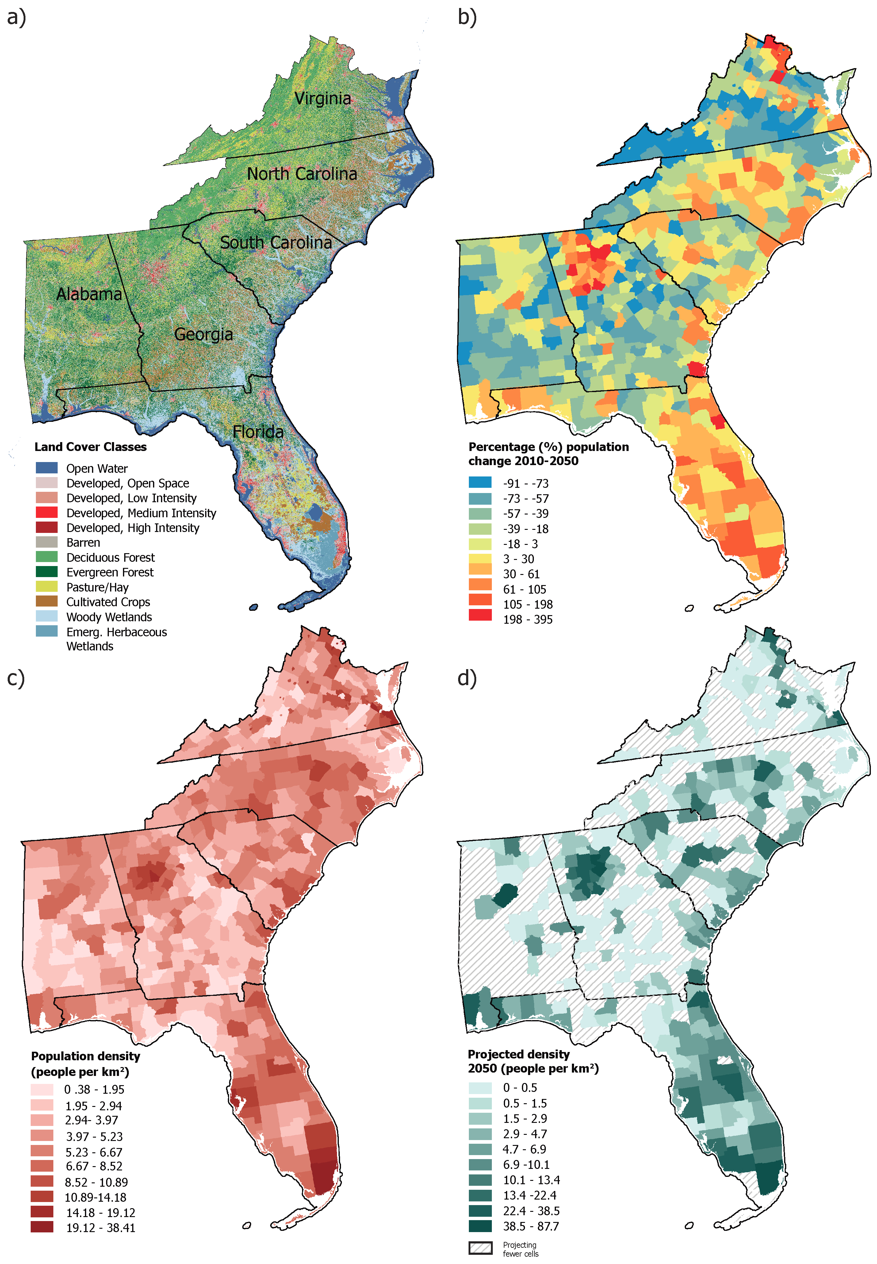
In this paper, we simulate urbanization and landscape change at high resolution across the South Atlantic States (SAS) region of the United States and evaluate the loss of productive lands and ecologically significant areas under Status Quo (SQ) and Infill urban growth scenarios using the FUTURES model [21]. FUTURES (FUTure Urban-Regional Environment Simulation) is a new user-friendly, open source geospatial computer model for simulating urbanization and landscape fragmentation [28]. It simulates landscape change based on demand for development, local development suitability factors, and a stochastic patch-growing algorithm (PGA). Recent advances to the model leverage parallel computing to produce multi-level projections over large spatial extents at fine granularity. We apply FUTURES to investigate the SAS, a region experiencing rapid population growth and increasing urbanization. We evaluate changes in land use, farmland, and ecologically significant areas that provide valuable wildlife corridors and habitat. Our overarching goal is to demonstrate a framework for simulating alternative futures of urban development at high resolution over a large extent to better understand the cumulative land change impacts of different urban growth strategies.

2. Methods

2.1. Study Area

Although almost entirely characterized by a temperate oceanic climate, the SAS region (Figure 1) is highly ecologically diverse. Home to a population of 55.6 million people [29] that is expected to reach 87.5 million by 2050 (ICLUS v1.3 Population Projections; USEPA, 2007), urban growth is projected to alter ecological and land systems in the coming decades. One of the most species-rich regions outside of the tropics, the SAS is also home to declining and endangered species, including previously dominant longleaf pine (Pinus palustris), sea turtles (e.g., Lepidochelys kempii), and the Red-cockaded Woodpecker (Picoides borealis) [8]. Added to this already complex urban-environmental challenge is the continuing urbanization of agricultural and amenity lands that are important for sustaining local economies and well-being [4].

Development patterns within the region are diverse, ranging from relatively undeveloped rural lands to sprawling suburban housing developments (e.g., Atlanta) and densely built, impervious urban areas (e.g., Miami). In general, new urban growth has abutted road networks, and can be characterized as low-density and sprawling [8]; however, demands for minimizing commuting times to central business districts (CBD), the rediscovery of urban cores as creative and lifestyle hubs [30], and increased environmental awareness promise new urban growth strategies focused on clustering and infill [31]. Foresight of the impacts of different development strategies would enable local and regional policymakers to better design urban developments that maintain vital ecosystems while supporting urban population ecosystem service demands [1].

2.2. Model Parameterization, Calibration and Validation

We project urban growth from 2010 to the year 2050 for the entire six-state region at 30 m pixel resolution. While economic and demographic projections indicate there is considerable demand for housing, industrial, and commercial developments and associated infrastructure in the coming decades [34,35], there is uncertainty regarding when, where, and the magnitude of urban growth across this highly diverse region. We approach this uncertainty by simulating plausible urbanization scenarios of growth trajectories [23] and replicating simulations (n = 50) to develop frequency maps of likely urban development locations. By comparing these simulations, we scope the different possible outcomes of this nonstationary, rapidly urbanizing system.

The FUTURES land change model simulates urban development using three submodels [20,21] including: (1) an urban development suitability surface derived from analysis of environmental factors (

Table 1. Description of independent variables included in estimated model of urban development suitability.

Name	Description	Units	Source
Urban land use	Classification of Urban land use (Class 21, 22, 23 & 24) from the NLCD product for 1992, 2001 and 2011	Presence/absence; 30 m cell	[32,36,37,38]
Development Pressure	Gravity calculation of 1 km Neighbourhood window of development over the reference years	Scale; 30 m cell	[32]; NLCD; FUTURES Calculation
Productive agriculture land (% 1 km${}^2$)	SSURGO high resolution classification of lands for agriculture(soil quality, soil moisture and topography)	Percentage; 30 m cell	[39]
Road density	(% 1 km${}^2$) Primary, secondary and connector road density	Percentage; 30 m cell	[40]
Woody Wetland (% 1 km${}^2$)	Percentage Emergent Herbaceous wetland within a 1 km neighborhood based on NLCD classification (Class)	Percentage; 30 m cell	[32]; NLCD
Emergent Herbaceous Wetlands (% 1 km${}^2$)	Percentage Emergent Herbaceous wetland within a 1 km neighborhood based on NLCD classification (Class)	Percentage; 30 m cell	[32]; NLCD
Forest land (% 1 km${}^2$)	Percentage forest within a 1 km neighborhood based on NLCD classification  (Class)	Percentage; 30 m cell	[32]; NLCD
Slope	Euclidian distance to lakes and rivers	Percentage; 30 m cell	[32]; NLCD
Distance to protected lands	Euclidean distance to IUNC protected areas (e.g., Federal and State Parks and Federal Forest)	Distance 1km (log transformed); 30 m cell	[41]
Distance to lakes and rivers	Euclidean distance to lakes and rivers	Distance 1 km (log transformed); 30 m cell	[42]

); (2) estimates of land consumption based on historical land cover and population data, as well as, population projections; and (3) urban patch growth characteristics, calibrated on existing urban spatial patterns. These submodels work together to capture the patchy spatial structure of urban development that often characterizes North American urban growth due to competing land demands, complex landowner utility, and variable urban policy instruments.

2.2.1. Urban Development Suitability

Urban development suitability is based on regional analysis of the relationship between locations of urban growth occurring between 1992 and 2011 and the associated environmental drivers of this change (all input parameters are 30 m pixel where possible). We fit a multilevel mixed model, iteratively testing and estimating different explanatory variables where the location of new urban growth is the dependent, response variable, and the county is the level of random effect (Table 1). By including a random effect [21], each county has a unique intercept, which accounts for local probability of urban development. We identified new urban cells for the time period by comparing the USGS 1992/2001 retrofit land cover change product and the 2011 land cover dataset, resolving well-known classification discrepancies between the datasets [36,43]. We tested several spatial factors widely agreed to influence urban development, including proximity to amenities, road density, agricultural and forest potential, land use competition, slope, and percent wetlands. These variables are specified as fixed-effects in the model and do not vary across each county, influencing development suitability the same across the SAS. In addition, we included a development pressure variable which approximates how existing urban development influences new growth as a random effect. Development pressure is calculated using a distance-decay function that we tested over a range of distances to calibrate the mean influence of spatial proximity to existing urban areas. Each county receives a unique development pressure, influencing spatial-arrangements of urban development at this spatial level (sprawl vs. compact development). We allow development pressure to vary, as it captures drivers of development, such as different planning measures and governance, that influence patterns of development but which are difficult to capture over this large scale. During simulations, development pressure is updated with each year as a feedback resulting from new development. Using a dredge function applied to all variable combinations, we compared the Akaike Information Criterion (AIC) to identify the best performing model for producing the spatially-explicit urban development suitability (

Table 2. Mixed effect model estimates for development suitability. Random effects are calculated per county (n = 573) with considerable variation between probability of development for the county (intercept) and the importance of development pressure across counties.

Fixed Effects	Estimate(Std. Error)	Pr (>|z|)
Intercept	−0.05 (0.04)	0.177
Percent forest (1 km)	−2.25 (0.01)	<0.000
Percent herbaceous wetlands (1 km)	−0.78 (0.062)	<0.000
Distance to lakes and rivers (km); log transformed	−0.19 (0.01)	<0.000
Percent productive agriculture land (1 km)	−0.07 (0.01)	<0.000
Road density (1 km)	12.35 (0.06)	<0.000
Percent wooded wetlands (1 km)	−2.021 (0.02)	<0.000
Distance to protected areas (km); log transformed	−0.01 (0.00)	<0.000
Slope	−0.01 (0.00)	<0.000
Random effects	Variance	Std.Dev
Development pressure	0.419	0.648
County (dumb.)	0.001	0.032

).

2.2.2. Land Consumption

In addition to environmental drivers of urban growth, FUTURES mimics social influences on urban land change by estimating local land consumption rates consistent with existing urban structures. Land consumption is based on changes in both historical population and the urban footprint of infrastructure and buildings, and then projecting land demand based on expected population growth at the county level. Our projections of land demand assume logarithmic growth and use the IPCC (Nakicenovic et al., 2000) Climate and Land-Use Scenarios (ICLUS) population estimates through 2050 [29]. This design allows for considering both path dependency of urban planning and increasing populations that match trends in densification (Figure 1). The IPCC ICLUS population projections are based on the SRES (Special Report on Emissions Scenarios) scenarios of likely demographic, economic, and governance changes over the coming decades [33]. We selected the A2 scenario as it projects the most dramatic population increase, best approximating the rapid growth occurring in the SAS region. The scenario assumes relatively slow demographic transition and slow convergence in regional fertility patterns that result in accelerating population growth in the largest urban centers of the SAS. By using the IPCC ICLUS projections we avoided the methodological inconsistencies and availability issues of population data offered by different state governments.

2.2.3. Urban Patch Growth

We calibrated urban growth patterns using representative, observed urban patch sizes and simulated urbanization using FUTURES stochastic patch growing algorithm. The algorithm stochastically selects a patch size from a patch library and then attempts to seed random locations across the defined developable landscape (i.e., county). When a seed’s random probability (0–1) exceeds the local development suitability probability, an urban patch is grown [21]. This model design accounts for local environmental factors that influence development while also approximating the unpredictable social drivers of urban growth. For example, reluctance to sell or develop in certain areas due to local factors is captured through the stochastic patch growing algorithm. While the social components of urban growth are considerably more complex at local scales compared to the stochastic processes simulated with the patch growing algorithm, the difficulty of efficiently capturing these key drivers across large extents necessitates a generalized approach [18].

In order to simulate urban development at high resolution over this large extent, we modified FUTURES to increase computational efficiency in two distinct ways that impact model functionality [44]: (1) we used a master–worker parallelization to increase computational speeds, where the model coordinates and independently allocates cells within each county without considering neighboring development pressure across county lines [44]; (2) we limited the number of iterations in the search for suitable developable locations. If the patch growing algorithm is unable to find a suitable cell after 100 attempts (this is commonly unregulated in the FUTURES model), development in that county is discontinued until the next year. This modification increased efficiency for individual workers and reduced computational time while likely increasing the importance of development suitability for seed selection [44]. The total duration of a model simulation (single run) using annual time steps to the year 2050 was approximately 3 h.

Validation of model projections is based on comparing our simulation estimates to observed data. We simulated urban growth from 1992 to 2011 (n = 19 years) and assessed correspondence to observed urban development patterns, which is a common approach for validation of land change projections [45,46]. We calculated the Kappa simulation (Ksim) statistic over 10 replicate simulations. Ksim measures map correspondence using a confusion matrix that controls for the high amount of persistence that inflates regular kappa measurements (see Appendix A for details). Persistence is prevalent in our study region, as a majority of the SAS remains unchanged over the simulation.

We furthermore evaluated pattern accuracy using a landscape similarity index (LSI) [14], for a combined measure indicating how well patches of simulated urban development mimic the spatial structure of observed urban growth. Using FRAGSTATS [47,48], we calculated: (1) number of urban patches (NP); (2) largest patch index (LPI); (3) mean Euclidean nearest-neighbor distance (ENN_MN); and (4) mean perimeter-area ratio (PARA_MN) for the reference year 2011 and the simulation runs (n = 10 years; 1992–2011). NP and LPI estimate the number and size of patches, while ENN_MN measures the distribution of patches, and PARA_MN evaluates patch shape and complexity. We also estimated total pattern-level similarity (LSI) by calculating the average of the absolute difference (%) between simulated and observed development for these metrics:

$$LSI=1-\frac{1}{4}\sum _i\Delta li,$$

(1)

$$\Delta li=\frac{|l_{i,s}-l_{i,o}|}{l_{i,o}}\ast 100;\dots \dots .NP,ENN\_MN,PARA\_MN,LPI,$$

(2)

where l_i,s and l_i,o are values of i-th landscape metrics derived from the simulated pattern and the observed pattern, respectively; $\Delta$li is the normalized difference of the i-th pair of simulated and observed landscape metrics. The large extent of the study area necessitated pattern accuracy assessments for randomly located subregions across the SAS (Figure 2). We sampled twenty, 100 km${}^2$ regions (10 km * 10 km) that crossed county boundaries and contained different regional geographic characteristics.

2.3. Scenarios of Urban Development

We projected urban development given (1) Status Quo (SQ) and (2) Infill scenarios of urban growth, and furthermore, quantified the frequency of development over 50 simulation replicates. This allowed for evaluating the plausibility of development over the stochastic simulation replicates, and accounted for the uncertainty that urban development occurs in a specific location at this resolution (30 m). Our baseline, SQ scenario is parameterized, based on land suitability estimated from historical development patterns, in the observed urban configuration (as described above). The urban Infill scenario modifies development probabilities relative to the SQ [21], increasing the chance that new developments are located near existing urban development, much like a land use plan that discourages or limits the possibility of sprawl. This modification is achieved through the FUTURES incentive parameter, which alters the base development probability of the SQ scenario using a spatially dependent power function ($P\left(d\right)=d^{\frac{1}{4}}$, where d is initial probability of development). This transforms the development probability surface and increases the likelihood of new development being located near existing development, resulting in more compact urban patches [21].

2.4. Land Change Evaluation under Status Quo and Infill Scenarios

We estimated the loss of productive agricultural land, cropland type, and ecologically significant areas under the simulated land change scenarios. This was achieved by intersecting frequency maps of projected urban development with land use, cropland type, and agricultural suitability data (USDA, 1995) (Appendix B, Figure A5). We furthermore evaluated probable impacts to biodiversity and cultural amenities, estimating changes on lands of ecological significance [49] (Appendix B, Figure A4).

3. Results

3.1. Model Parameterization, Calibration and Validation

Model results indicated that proximity to amenities (e.g., protected areas, water bodies), and road density positively influenced urban development across the SAS. Measures of agricultural and forest potential, competing land uses, percent wetlands, and slope are negatively associated with urban development, as factors that likely increase construction costs (

Table 3. Percent agreement between simulations (mean) and observed development based on the landscape similarity index (LSI), which evaluates the number of urban patches (NP); largest patch index (LPI); mean Euclidean nearest-neighbor distance (ENN _MN); and (4) mean perimeter–area ratio (PARA_MN). Low similarity is observed in only four sample areas (e.g., zones 8, 10, 18, 20).

	Actual Urban Pattern				Simulated Urban Pattern
Sampling Area	NP	LPI	PARA _MN	ENN _MN	NP	LPI	PARA _MN	ENN _MN	LSI
1	0.107	0.007	0.010	0.163	0.189	0.025	0.011	0.148	92.86%
2	0.074	0.015	0.128	0.403	0.151	0.028	0.118	0.373	84.54%
3	0.132	0.021	0.102	0.261	0.207	0.039	0.096	0.244	87.11%
4	0.32	0.052	0.062	0.134	0.373	0.079	0.064	0.127	85.95%
5	0.385	0.09	0.063	0.194	0.428	0.122	0.069	0.182	81.74%
6	0.34	0.009	0.07	0.198	0.39	0.046	0.068	0.186	84.59%
7	0.179	0.02	0.076	0.281	0.247	0.043	0.072	0.26	86.11%
8	0.633	0.379	0.089	0.148	0.638	0.404	0.121	0.146	68.79%
9	0.255	0.011	0.069	0.228	0.315	0.04	0.066	0.212	85.97%
10	1.115	0.05	0.106	0.095	1.071	0.127	0.108	0.096	66.44%
11	0.461	0.029	0.067	0.146	0.497	0.075	0.068	0.139	82.43%
12	0.294	0.005	0.053	0.195	0.352	0.037	0.051	0.18	86.38%
13	0.316	0.125	0.069	0.162	0.366	0.148	0.077	0.154	83.25%
14	0.113	0.19	0.034	0.274	0.186	0.189	0.05	0.252	84.72%
15	0.003	0.013	0.018	0.402	0.091	0.021	0.018	0.364	89.1%
16	0.25	0.037	0.04	0.254	0.311	0.064	0.042	0.233	85.48%
17	0.192	0.057	0.038	0.215	0.26	0.077	0.041	0.197	87.49%
18	0.503	0.006	0.046	0.274	0.532	0.061	0.048	0.251	79.22%
19	0.145	0.016	0.058	0.278	0.218	0.034	0.055	0.255	87.66%
20	1.884	0.455	0.022	0.08	1.736	0.549	0.075	0.08	39.8%

). Development pressure varied by county (Appendix B, Figure A3), resulting in the spatial proximity of existing urban areas having differing influences on new development. For example, high development pressure that results in increased chance of compact development patterns are found in the central core of highly urbanized counties (e.g., Atlanta, GA, USA and Raleigh, NC, USA), as well as coastal and mountainous areas where there are geographic constraints and environmental amenities that shape compact patterns of development proximate to these features. Conversely, counties with low development pressure that results in lower probability of compact development patterns are found in rural and suburban areas throughout the SAS (Appendix B, Figure A3) .

Validation results indicated a well fit model of urbanization after accounting for persistence (Ksim 0.42). Kappa measures between 0.20–0.40 are similar to other land change models [14] (e.g., GEOMOD, LANDUSE Modeller, CLUE, SLUETH). Moreover, there was high agreement between the multiple (n = 10) hindcasting simulations (std dev 0.0021). While overall pattern accuracy was well projected with a total landscape similarity index of 81.48%, averaged over the twenty randomly chosen sample sites, there was spatial heterogeneity in model projections over these areas (LSI measures ranging between 39.8–92.7%; Table 3). For example, LSI results in the peri-urban area of Mobile, AL, USA (zone 20) indicated poor agreement, simulating highly patchy growth instead of the actual compact growth (Table 2). Still, high correspondence between simulated and observed development in the majority of the regions suggests reasonable overall accuracy.

3.2. Projections of Urban Development

Our simulations project an additional 7449.9 km${}^2$ (15.0% increase; std.dev 0.9 km${}^2$) of urban development in the SAS over the 2011–2050 period given the status quo growth scenario, and 7271.74 km${}^2$ (14.8% increase; std.dev 0.5 km${}^2$) based on an infill strategy. The difference in total increase in urban impervious between the scenarios (178.2 km${}^2$) is due to constraints on suitable locations for development in the infill strategy. Frequency maps of the 50 simulation replicates reveal varying patterns of development between counties (Figure 3; Appendix Figure A3). Development in counties with large urban centers (e.g., Figure 3, the counties of Hillsborough, FL, USA and Loudoun, VA, USA) and along the coast is highly concentrated and adjacent to factors favorable to growth (e.g., proximity to amenities, higher road densities), whereas new development is more dispersed and randomly located in other counties (e.g., Figure 3, the rural portion of the counties of Cherokee, GA, USA and Wake, NC, USA). Development patterns also differ between the scenarios as specified in model implementation. For example, the Status Quo scenario results in dispersed development across counties, whereas the Infill strategy allocates new development in close proximity to existing development and roads (Figure 3, Figure A1 and Figure A2).

3.3. Land Changes under Status Quo and Infill Scenarios

Changes in land cover as a result of simulated development, including net losses of cropland and important ecological areas, were similar in both the SQ and Infill scenarios. However, notable differences occurred in some land cover/use categories due to the different spatial patterns of cell allocation between scenarios (Figure 3). For example, loss of emergent herbaceous wetlands, cultivated crops, shrub/scrub lands, evergreen and deciduous forests are greater in the SQ scenario compared to the Infill scenario (Figure 4). Conversely, barren land, woody herbaceous wetlands, and pasture are conserved on average with more frequency in the SQ scenario compared to Infill. Losses varied for specific crops, with peach orchards, for example, under greater threat from infill, and sugarcane and corn under the SQ scenario. Across the SAS region, over twice as much of highly suitable agricultural land is consumed in the SQ scenario (loss of 2.97%) as compared to the Infill scenario (loss of 1.23%). Ecologically significant areas are equally threatened under both scenarios in terms of net loss of area, albeit with different fragmentation patterns due to differences in developed cell allocation during the simulations (Figure 5). High and medium ecological conservation priority areas will be reduced by 2.0–2.1% and 1.6–1.5% for SQ and Infill scenarios, respectively. Patterns of development and landscape change are, however, qualitatively different between scenarios with increased fragmentation of ecological priority areas under the SQ urban development scenario (Figure 5).

3.4. Pattern Evaluation

We compared frequency maps between the SQ and Infill scenarios and found that, as expected, urban sprawl increased under the SQ scenario in urban areas throughout the SAS (Figure 6). New development in polycentric urban areas, for example, Atlanta, Georgia, and the Triangle (Raleigh, Durham, and Chapel Hill, in North Carolina), occurred primarily on the lands between CBDs. New development in coastal areas, for example, Charleston, SC, USA, and Savannah, GA, USA, is characterized by directional, concentric, urban growth patterns radiating from these water bodies. The Infill scenario produced less patchy, more concentric development patterns with the majority of new development located adjacent to the existing urban footprint.

4. Discussion

We present a methodology for assessing broad scale impacts of likely future urban growth using the FUTURES model. Traditionally, land change and urban modelling for large regions have been conducted at coarse resolution or through brute force due to computational demands and limitations [6,15]. Our application illustrates the challenge of simulating land change at relatively high resolution (30 m) over a large extent (six U.S. states). Achieving high resolution projections of land change over multiple jurisdictional areas is necessary for accurately assessing the cumulative impacts of land change at resolutions that match ecological and social processes. For example, such simulations can help in local planning for recreational areas, as well as understanding how agricultural production will be impacted given different planning strategies.

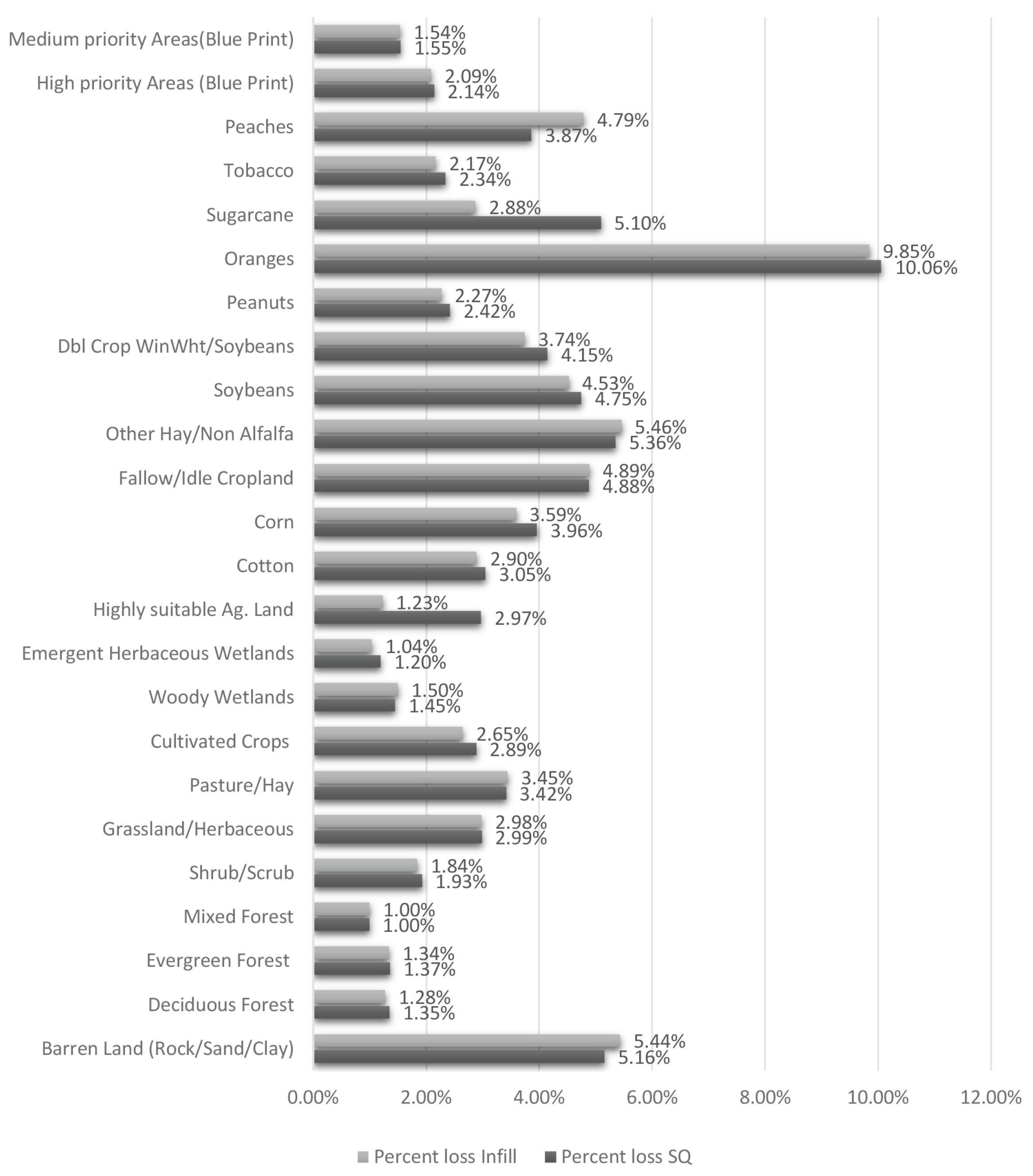
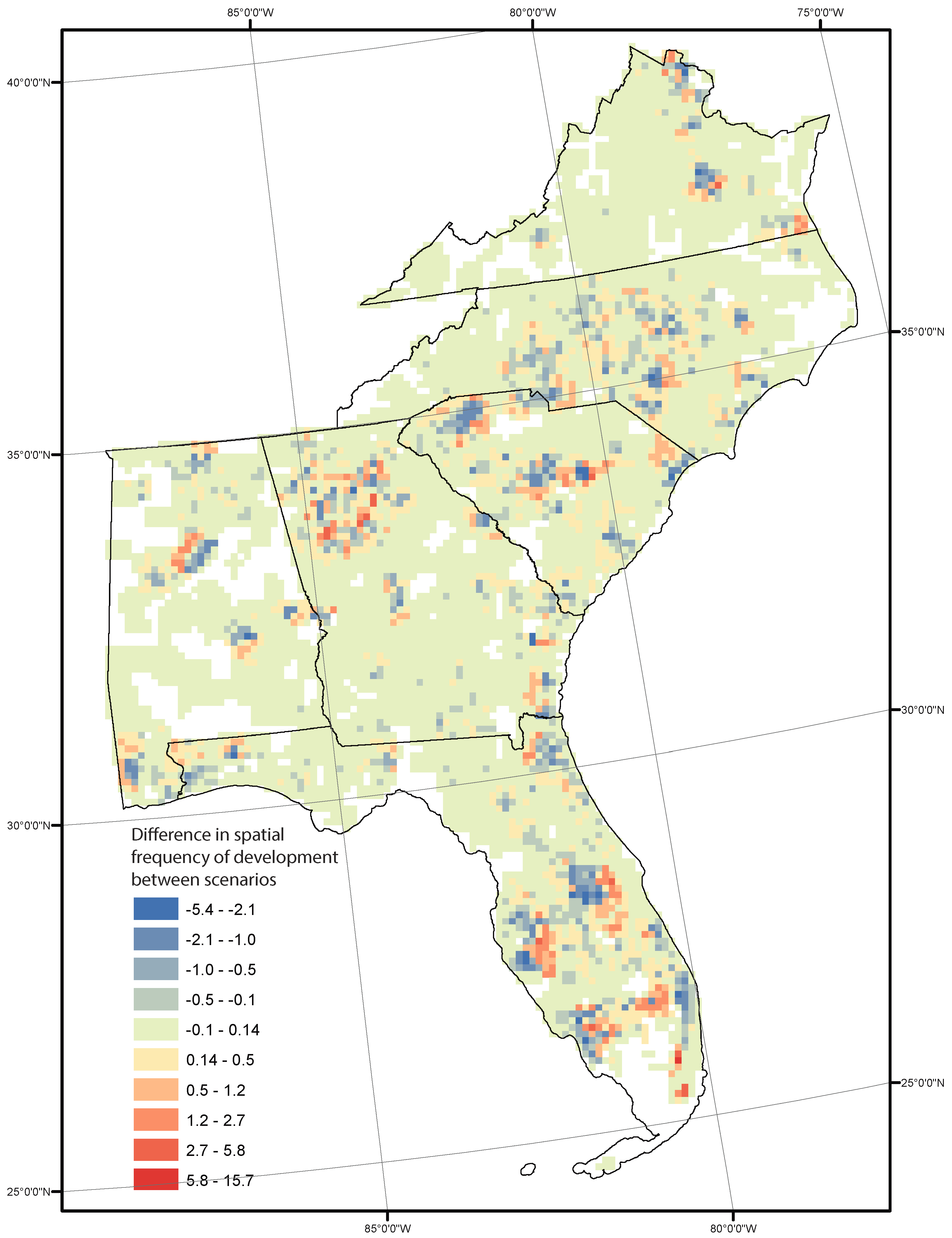
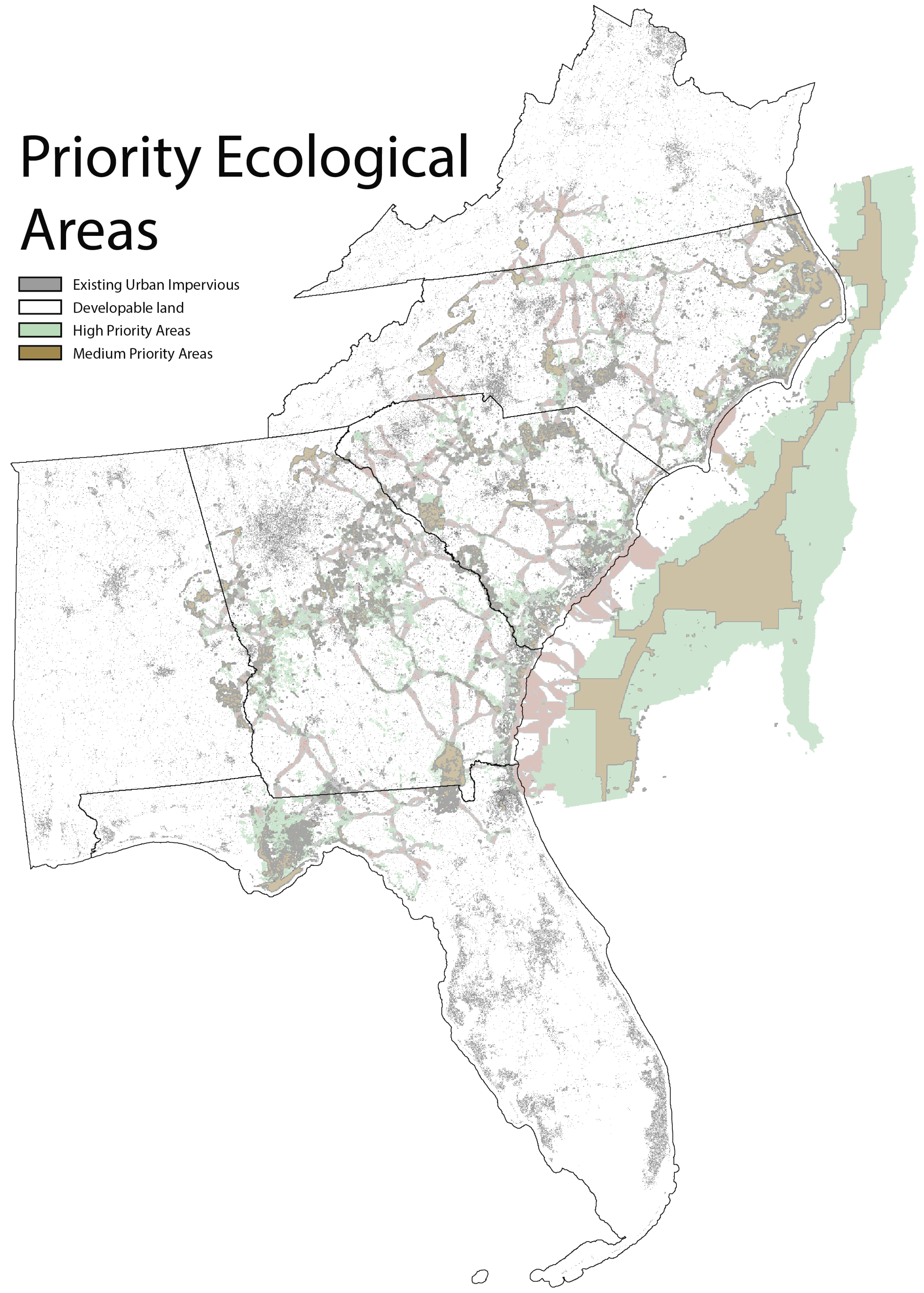
Our results indicate that important ecological areas, forest and farmland are vulnerable to urban development across the SAS over the coming decades. While overall losses are similar between the Infill and SQ scenarios (Appendix B

Table A1. Land use/cover change (average simulated 2050/total 2011) under the Status Quo and Infill urban growth scenarios.

		Status Quo		Infill
Land Area	Current Total (NLCD Estimate)	Total (km${}^2$)	Diff.	Total (km${}^2$)	Diff.
Total Impervious surface (NLCD 21, 22, 23, 24 categories, excluding roads and urban areas in protected  areas)	49,161.48	56,611.38 (std. dev. 0.937)	7449.9 (15.0% increase)	56,433.22 (std. dev 0.504)	7271.74 (14.8% increase)
Barren Land (Rock/Sand/Clay)	2844.782	2698.02 (0.001)	146.76 (−5.16%)	2149.54 (0.004)	154.62 (−5.44%)
Deciduous Forest	146,452.8	144,474.11 (0.002)	1978.66 (−1.35%)	138,053.06 (0.008)	1868.10 (−1.28%)
Evergreen Forest	123,619.3	121,930.42 (0.001)	1688.88 (−1.37%)	116,145.79 (0.009)	1662.11 (−1.34%)
Mixed Forest	24,262.81	24,021.33 (0.001)	241.488 (−0.10%)	23,174.60 (0.002)	242.02 (−0.10%)
Shrub/Scrub	55,665.81	54,593.01 (0.003)	1072.80 (−0.19%)	51,060.97 (0.01)	1024.12 (−0.18%)
Grassland/Herbaceous	32,747.83	31,769.54 (0.00)	978.29 (−2.99%)	28,353.77 (0.01)	977.24 (−2.98%)
Pasture/Hay	77,658.3	75,002.46 (0.00)	2655.83 (−3.42%)	65,628.78 (0.01)	2675.36 (−3.45%)
Cultivated Crops	57,840.89	56,170.32 (0.00)	1670.57 (−2.89%)	50,955.45 (0.01)	1531.32 (−2.65%)
Woody Wetlands	102,494.2	101,005.34 (0.00)	1488.84 (−1.45)	95,581.65 (0.01)	1537.35 (−1.50%)
Emergent Herbaceous Wetlands	25,545.58	25,240.13 (0.00)	305.45 (−1.20%)	24,348.28 (0.00)	266.28 (−1.04%)

and

Table A2. Change to farmland and ecologically significant areas (average simulated 2050/total 2011) under the SQ and Infill urban growth scenarios.

		Status Quo		Infill
Land Area	Current Total (NLCD Estimate)	Total (km${}^2$)	Diff.	Total (km${}^2$)	Diff.
Highly suitable agricultural land (SSURGO) that is available for cultivation (i.e., not topped by an impervious  layer)	108,523.21 km${}^2$	105,295.1 (std. dev. 0.55)	3228.12 (−3.0%)	107,187.54 (std. dev. 0.54)	1335.67 (−1.2%)
Cotton	14,383.9	13,945.36 (0.56)	438.53 (−3.05%)	13,967.34 (0.09)	416.56 (−2.99%)
Corn	9764.004	9377.37 (0.17)	386.63 (−3.96%)	9413.00 (0.25)	351.00 (−3.59%)
Fallow/Idle Cropland	8561.428	8143.32 (0.06)	418.11 (−4.88%)	8142.76 (0.13)	418.67 (−4.89%)
Other Hay/Non Alfalfa	7830.199	7410.48 (0.38)	419.72 (−5.36%)	7402.69 (0.11)	427.50 (−5.46%)
Soybeans	6708.426	6389.75 (0.18)	318.68 (−4.75%)	6404.71 (0.16)	303.72 (−4.53%)
Dbl. Crop Winter Wheat/Soybeans	4404.217	4221.37 (0.13)	182.84 (−4.15%)	4239.33 (0.14)	164.89 (−3.74%)
Peanuts	4180.232	4079.02 (0.08)	101.21 (−2.42%)	4085.30 (0.07)	94.93 (−2.27%)
Oranges	4017.964	3613.77 (0.48)	404.20 (−10.06%)	3622.31 (0.35)	395.66 (−9.85%)
Sugarcane	1690.131	1604.00 (0.02)	86.13 (−5.10%)	1641.518 (0.04)	48.62 (−2.88%)
Tobacco	115.7382	113.03 (0.05)	2.71 (−2.34%)	113.23 (0.02)	2.51 (−2.17%)
Peaches	67.0041	64.42 (0.00)	2.59 (−3.87%)	63.79 (0.01)	3.21 (−4.79%)
Sugarcane	1690.131	1604.00 (0.02)	86.13 (−5.10%)	1641.518 (0.04)	48.62 (−2.88%)
Tobacco	115.7382	113.03 (−0.05)	2.71 (−2.34%)	113.23 (0.02)	2.51 (−2.17%)
Peaches	67.0041	64.42 (0.00)	2.59 (−3.87%)	63.79 (−0.01)	3.21 (−4.79%)
High Priority Areas	139,115.54	1,361,358.7 (4.68)	2979.66 (−2.14)	1,362,114.25 (3.62)	2904.12 (−2.09)
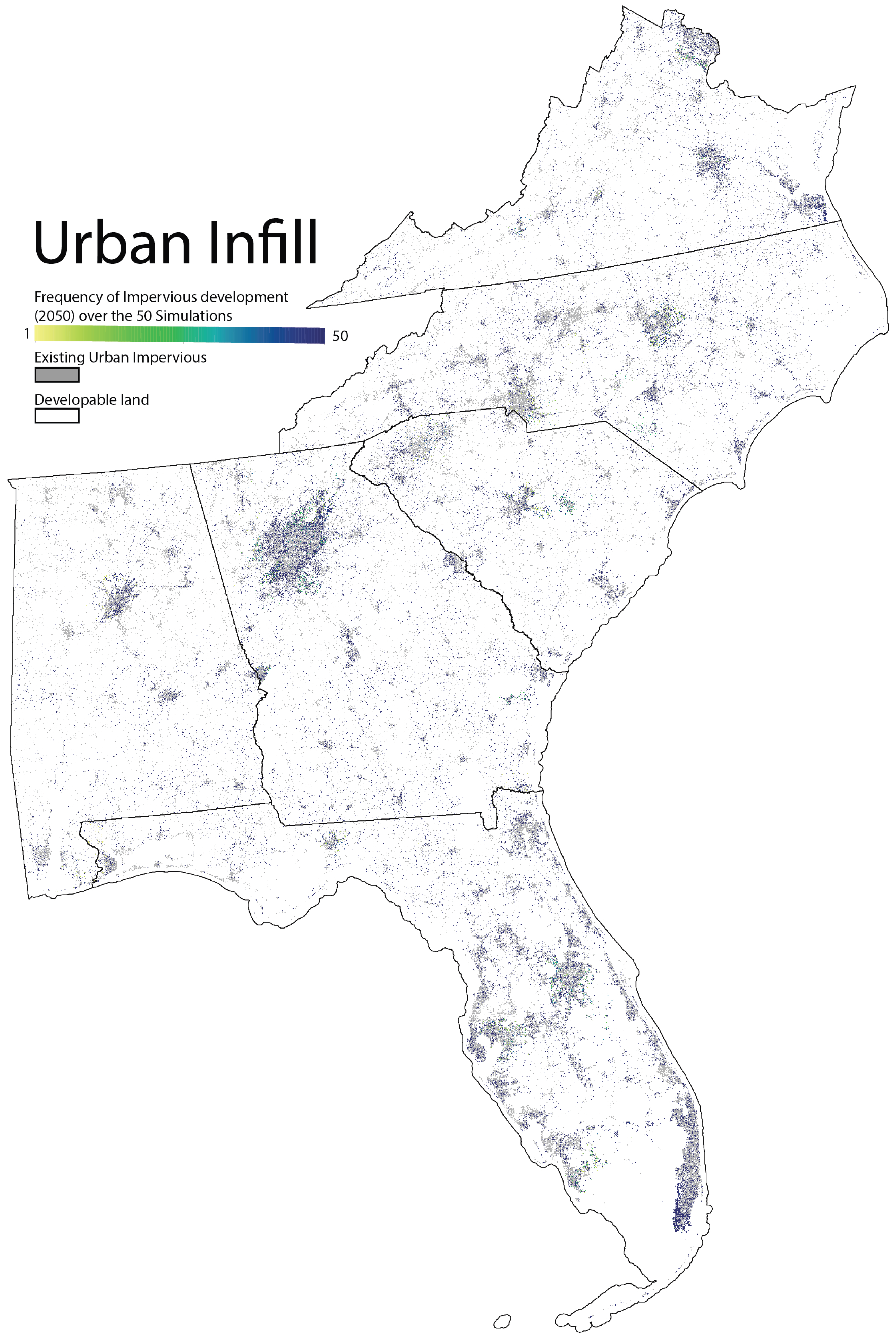
Medium Priority Areas	125,907.0147	1,239,538.5 (5.84)	1953.16 (−1.55)	1,239,650.39 (2.65)	1941.98 (−1.54)

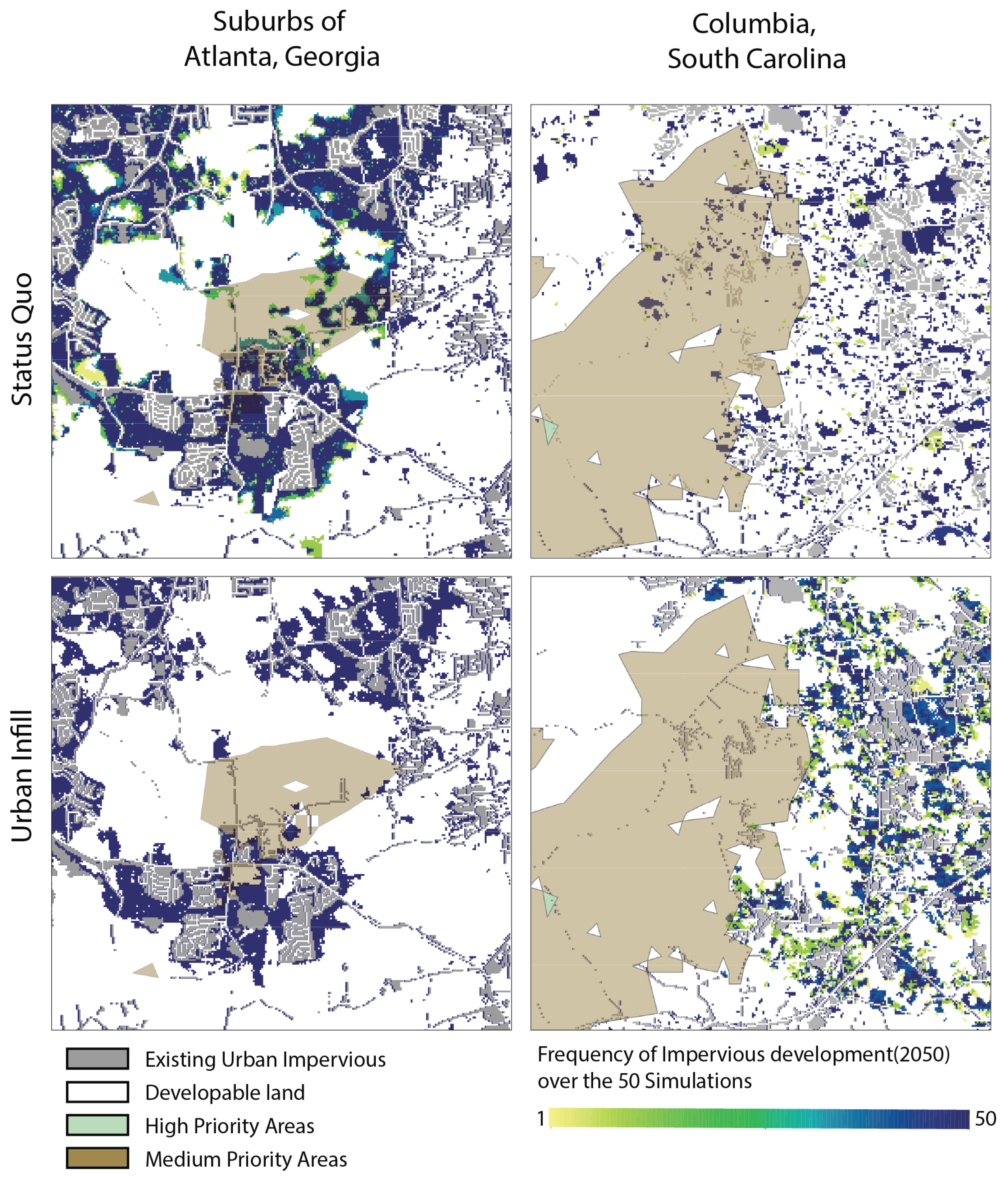
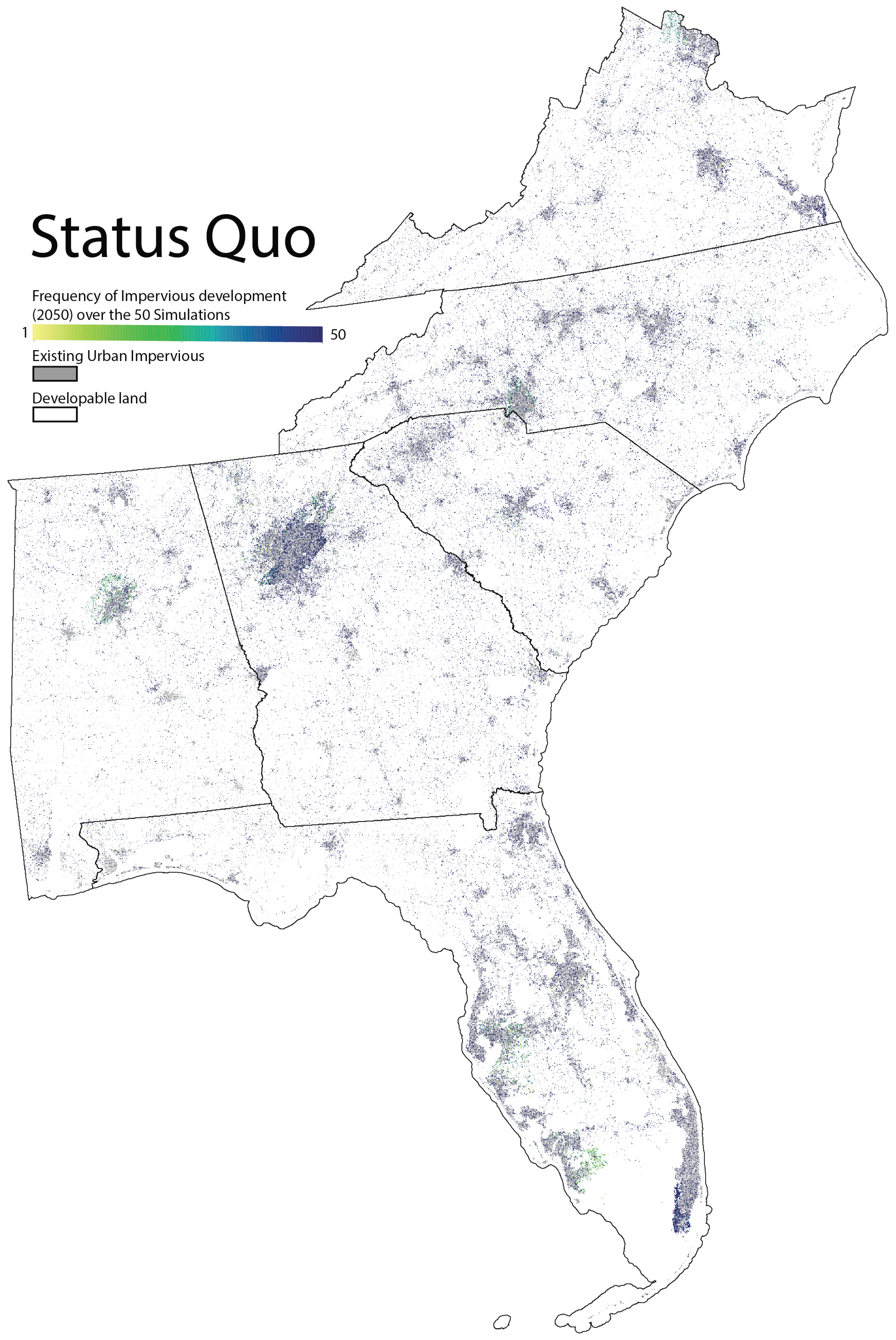
), differences in development patterns and local variation in land cover/use result in different land change impacts. For example, the greater loss of productive peach growing lands in the Infill scenario is due to the high concentration of peach orchards in close proximity to growing medium-sized rural centers in Georgia and South Carolina (Appendix B Table A2, Figure A1 and Figure A2). The low concentration of productive farmlands in close proximity to major urban centers like Miami, Atlanta, and Birmingham, conversely, results in greater losses in the SQ scenario (Appendix B Figure A1 and Figure A2), as development occurs further from the urban fringe. Despite losses in non-urban land use, the more compact development patterns resulting from the Infill scenario spare larger, contiguous patches of forests and agricultural land compared to the patchy, dispersed, patterns of SQ development in the SAS [3].

The different patterns of urbanization and landscape change will likely influence the actual flow of ecosystem services in ways that are obscured at large regional scales. Ecologically, the dispersed patterns produced by the SQ scenario will additionally result in changes to lands between urban developments (e.g., forests, agricultural land). For example, the development of parks and greenways on these lands, that include infrastructure for residents of developed communities, will result in additional fragmentation of habitat. Farmland fragmented by the SQ growth will likewise be altered as agricultural production becomes less viable due to changes in parcel configuration. Considering trade-offs related to pattern requires fine scale and contextual information that is difficult to summarize at larger scales [5] and likely requires improved understanding of how pattern influences the flow of ecosystem services.

4.1. Challenges Getting the Pattern Correct

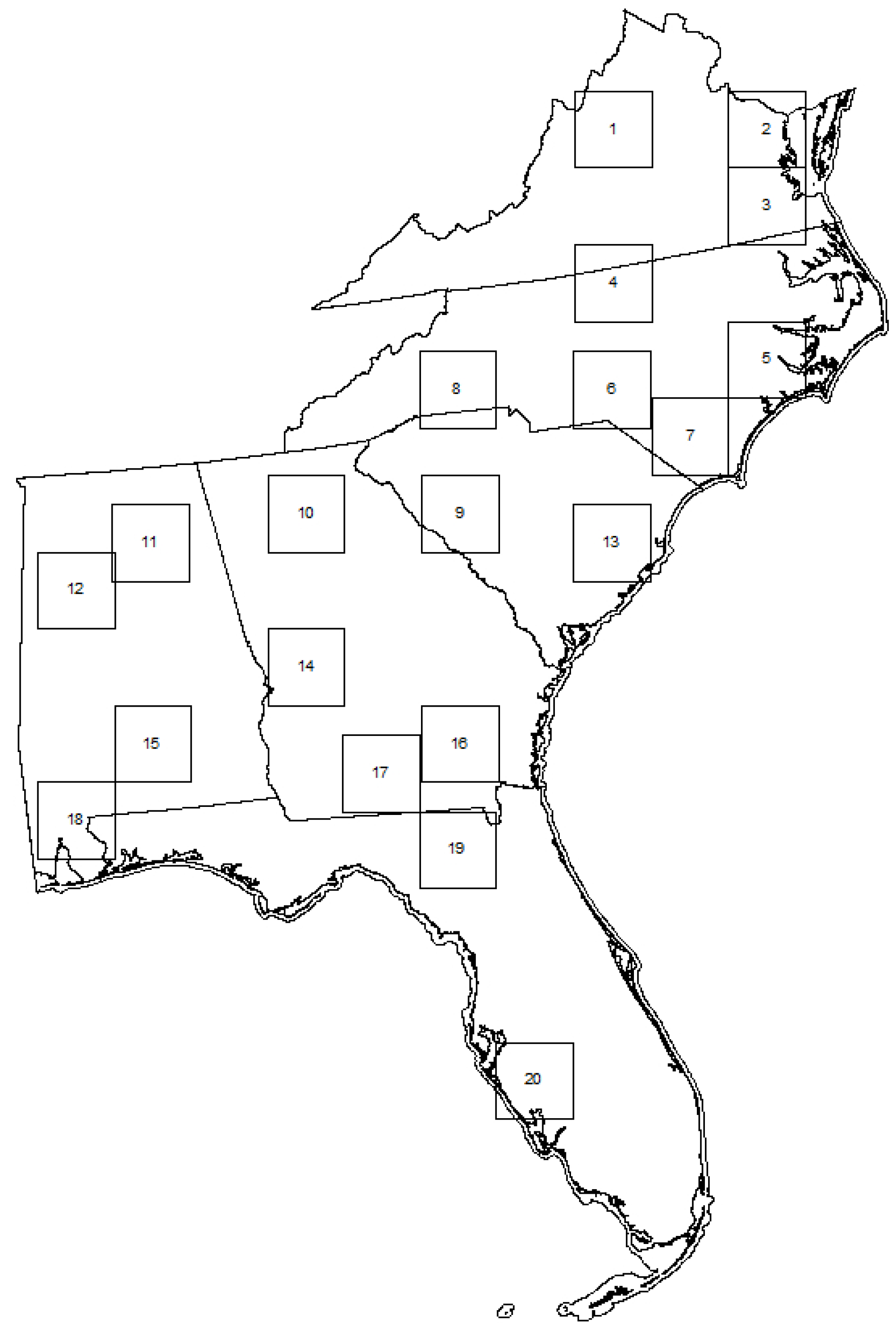
Our validation, based on hindcasting simulations between 1992–2011, showed reasonable agreement with observed urban development in the 2011 reference year, comparable to other land change model accuracies [14]. Moreover, LSI measures indicated high correspondence between simulated and observed development patterns in a majority of the sampled regions. While some areas were less well projected, this is to be expected and reflects both the inherent heterogeneity of urban development and the challenge of estimating future urbanization at large scales and fine resolution.

As approximations of complex systems, urban and land change models are simplified abstractions, not fully representing patterns of development nor projecting the specific locations of change with complete accuracy. While increasing the sophistication of model parameterization to better match local processes and improve accuracy is an important goal for land change science [45], there are trade-offs for simulations at high resolution over large extents. Traditionally, land change for large regions has been done using cellular automata (CA) models (e.g., CLUE, SLEUTH) with simplified inputs that can be obtained for large extents and using simple geographic rules that are broadly applicable [8,15]. Agent-based models that include high levels of model complexity, however, are often better at mimicking local processes by incorporating behavioral drivers [18], resulting in increased local pattern simulation accuracy. The computational demands (local agent decisions) and data requirements (local model of behavior), however, means that it is rarely practical to use ABMs for simulating urbanization for large regions. The FUTURES model partially accounts for how local scale processes influence development by incorporating local estimates of land consumption, local urban growth models (i.e., county), and local estimates of how existing development impacts subsequent growth. Such an approach that combines both general models applicable over the entire geographic extent and local models that capture finer scale aspects of development is a promising methodology for simulations over large areas. Our parameterization of local factors influencing urban growth, embedded within a general model of urbanization, enabled us to increase computational efficiency while simulating new development with reasonable accuracy.

Similar developed locations in both the SQ and Infill scenarios over the 50 different simulations should be considered when interpreting the results. In this implementation of FUTURES, we used parallelization that increased model speed by simultaneously simulating urbanization within individual counties [44]. This process limited sites for possible new development (seed selection) compared to simulating change over several counties (the original design of FUTURES), and thereby, increased the chance that a specific set of highly suitable cells were repeatedly developed over the 50 simulation years. To solve this path dependent outcome, future implementations of the model will need to run experiments that identify larger regions (i.e., multiple counties) at which development is appropriate (e.g., Atlanta metro area); thereby improving the realism of the model projections, and balancing the computational requirements of simulating urban development over these larger areas.

Furthermore, while our results show promise, our choice of a 30 m resolution does increase uncertainty due to the granularity of our projections. For example, the site of a new building and its associated infrastructure, which is distinguishable at this resolution, is highly unpredictable. Our projections represent landscape-scale trends of urbanization processes rather than actual, site-specific outcomes, and this inherent spatial uncertainty should be considered when interpreting the results. Our chosen resolution matches the development of urban impervious surface over a broad range of land types (i.e., farm buildings, exurban development, new housing subdivision); however, it is unlikely to be practical for measuring the impact of some land use and ES trade-offs. For example, projecting the impacts on farmlands at this resolution is unlikely to be necessary, as conversion often occurs at coarser resolutions (i.e., parcel level). Within-parcel land change, however, will likely impact other ES that requires this fine-resolution projection (e.g., micro-ecology landscape aesthetics). Additional research into the appropriate scale and extent of study will be an important step for projecting land use and ES trade-offs over time. Promising nested modeling frameworks that simulate land change at multiple resolutions may additionally aid in projecting at appropriate scales for various ES [50]. Such simulations can be conducted at coarser resolutions in productive landscapes (i.e., timber and farmland), and finer resolutions in recreational and biodiverse areas where this scale of analysis is appropriate (see further discussion in the next section).

4.2. Addressing Scales Relevant to Social and Ecological Function

Modelling urban growth at high resolution is an important advancement in land change science as it will enable simulations that reflect the scales at which social and ecological functioning occurs and for which policy is designed. FUTURES, for example, mimics the development of subdivisions that are often a mixture of pervious and impervious surfaces, as well as single small urban structures (Figure 3; Appendix B Figure A1 and Figure A2). This better reflects the different fragmentation patterns occurring around urban areas and allows for improved evaluation of these development outcomes. For example, persistent urban greenspace around and within subdivisions might serve an important social function, providing natural areas for walking paths or be of ecological benefit, creating specific habitat for certain species [3,26]. Conversely, fragmentation may increase the cost of infrastructure and create a barrier for the movement of wildlife. In the context of agriculture, more contiguous patterns like those realized in an Infill scenario are likely more productive as there are fewer hindrances to the movement of large farming equipment and more efficient use of land. Such evaluations are only possible if land change models simulate different patterns of development at resolutions that match ecological and social functioning.

Similarly, large-scale outcomes of land change, modelled with high granularity, are important to consider as small changes can have large macro-scale impacts, for example, in food systems. The difference between a 3% (SQ) and a 1% (Infill) decrease in productive farmland in a highly productive agricultural area can have substantial impacts on regional and global food chains [51]. Our model implementation allows for the rapid evaluation of microscale change impacts at the macroscale.

Representing these microscale developments and macroscale impacts will likewise increase the plausibility of simulations, creating important buy-in from stakeholders. Land change models based exclusively on site suitability often result in concentric development patterns that, in the context of the multinodel development that typifies US growth, may be viewed with much skepticism. Representing the common leapfrog development pattern, even in the abstract sense due to limited accuracy, is important to present to policymakers familiar with urban growth. Simulating more plausible development patterns can potentially increase the need for considering urban growth patterns in urban design and planning. Likewise, providing evidence of the cumulative impacts of these local scale changes may increase coordination between regions and countries to implement land sparing strategies that protect the global food supply.

5. Conclusions

Land sharing and land sparing strategies of urban growth produce qualitatively different patterns of urbanization and landscape change that differentially impact agricultural and natural systems across the U.S. Land sparing or infill strategies can play an important role in preventing even greater fragmentation of forests, farmlands, and important wildlife habitat in the coming decades. Our application of FUTURES in the SAS region of the U.S. illustrates the challenges and opportunities for spatially-explicit land change models to help us better understand these processes and their cumulative impacts at high resolution and over large extents.

References

1. Bolund, P.; Hunhammar, S. Ecosystem services in urban areas. Ecol. Econ. J. Int. Soc. Ecol. Econ. 2008, 29, 293–301. [Google Scholar] [CrossRef]
2. Phalan, B.; Onial, M.; Balmford, A.; Green, R.E. Reconciling food production and biodiversity conservation: Land sharing and land sparing compared. Science 2016, 333, 1289–1291. [Google Scholar] [CrossRef] [PubMed]
3. Stott, I.; Soga, M.; Inger, R.; Gaston, K.J. Land sparing is crucial for urban ecosystem services. Front. Ecol. Environ. 2012, 13, 387–393. [Google Scholar] [CrossRef]
4. Brown, D.G.; Johnson, K.M.; Loveland, T.R.; Theobald, D.M. Rural Land-use Trends in the Conterminous United States, 1950–2000. Ecol. Appl. Publ. Ecol. Soc. Am. 2005, 15, 1851–1863. [Google Scholar] [CrossRef]
5. Pickard, B.; Gray, J.; Meentemeyer, R. Comparing Quantity, Allocation and Configuration Accuracy of Multiple Land Change Models. Land 2017, 6, 52. [Google Scholar] [CrossRef]
6. Radeloff, V.C.; Nelson, E.; Plantinga, A.J.; Lewis, D.J.; Helmers, D.; Lawler, J.J.; Polasky, S.; Withey, J.C.; Beaudry, F.; Martinuzzi, S.; et al. Economic-based projections of future land use in the conterminous United States under alternative policy scenarios. Ecol. Appl. Publ. Ecol. Soc. Am. 2012, 22, 1036–1049. [Google Scholar] [CrossRef] [PubMed]
7. Seto, K.C.; Güneralp, B.; Hutyra, L.R. Global forecasts of urban expansion to 2030 and direct impacts on biodiversity and carbon pools. Proc. Natl. Acad. Sci. USA 2012, 109, 16083–16088. [Google Scholar] [CrossRef] [PubMed] [Green Version]
8. Terando, A.J.; Costanza, J.; Belyea, C.; Dunn, R.R.; McKerrow, A.; Collazo, J.A. The Southern Megalopolis: Using the Past to Predict the Future of Urban Sprawl in the Southeast U.S. PLoS ONE 2014, 9, e102261. [Google Scholar] [CrossRef] [PubMed]
9. United Nations, Department of Economic and Social Affairs, and Population Division. World Population Prospects Highlights 2019. Available online: https://population.un.org/wup/Publications/Files/WUP2018-Report.pdf (accessed on 19 September 2019).
10. Pontius, R.G.; Boersma, W.; Castella, J.-C.; Clarke, K.; de Nijs, T.; Dietzel, C.; Verburg, P.H.; Lippitt, C.D.; McConnell, W.; Sood, A.M.; et al. Comparing the input, output, and validation maps for several models of land change. Ann. Reg. Sci. 2008, 42, 11–37. [Google Scholar] [CrossRef]
11. Kok, K.; van Vliet, M.; Bärlund, I.; Dubel, A.; Sendzimir, J. Combining participative backcasting and exploratory scenario development: Experiences from the SCENES project. Technol. Forecast. Soc. Chang. 2011, 78, 835–851. [Google Scholar] [CrossRef]
12. Westhoek, H.J.; van den Berg, M.; Bakkes, J.A. Scenario development to explore the future of Europe’s rural areas. Agric. Ecosyst. Environ. 2006, 114, 7–20. [Google Scholar] [CrossRef]
13. Verburg, P.H.; van Berkel, D.B.; van Doorn, A.M.; van Eupen, M.; van den Heiligenberg, H.A. Trajectories of land use change in Europe: A model-based exploration of rural futures. Landsc. Ecol. 2014, 25, 217–232. [Google Scholar] [CrossRef]
14. Pickard, B.R.; Van Berkel, D.; Petrasova, A.; Meentemeyer, R.K. Forecasts of urbanization scenarios reveal trade-offs between landscape change and ecosystem services. Landsc. Ecol. 2017, 32, 617–634. [Google Scholar] [CrossRef]
15. Verburg, P.H.; Overmars, K.P. Combining top-down and bottom-up dynamics in land use modeling: Exploring the future of abandoned farmlands in Europe with the Dyna-CLUE model. Landsc. Ecol. 2009, 24, 1167–1181. [Google Scholar] [CrossRef]
16. Kaza, N.; BenDor, T.K. The land value impacts of wetland restoration. J. Environ. Manag. 2007, 127, 289–299. [Google Scholar] [CrossRef] [PubMed]
17. Fang, Y.; Jawitz, J.W. High-resolution reconstruction of the United States human population distribution, 1790 to 2010. Sci. Data 2005, 5, 180067. [Google Scholar] [CrossRef] [PubMed]
18. Koch, J.; Dorning, M.A.; Van Berkel, D.B.; Beck, S.M.; Sanchez, G.M.; Shashidharan, A.; Meentemeyer, R.K. Modeling landowner interactions and development patterns at the urban fringe. Landsc. Urban Plan. 2007, 182, 101–113. [Google Scholar] [CrossRef]
19. Magliocca, N.; McConnell, V.; Walls, M. Exploring sprawl: Results from an economic agent-based model of land and housing markets. Ecol. Econ. J. Int. Soc. Ecol. Econ. 2015, 111, 114–125. [Google Scholar] [CrossRef]
20. Dorning, M.A.; Smith, J.W.; Shoemaker, D.A.; Meentemeyer, R.K. Changing decisions in a changing landscape: How might forest owners in an urbanizing region respond to emerging bioenergy markets? Land Use Policy 2005, 49, 1–10. [Google Scholar] [CrossRef]
21. Meentemeyer, R.K.; Tang, W.; Dorning, M.A. FUTURES: Multilevel simulations of emerging urban–rural landscape structure using a stochastic patch-growing algorithm. Ann. Assoc. Am. Geogr. 2013, 103, 785–807. [Google Scholar] [CrossRef]
22. Martinuzzi, S.; Radeloff, V.C.; Joppa, L.N.; Hamilton, C.M.; Helmers, D.P.; Plantinga, A.J.; Lewis, D.J. Scenarios of future land use change around United States’ protected areas. Ecol. Biol. Conserv. 2015, 184, 446–455. [Google Scholar] [CrossRef]
23. Rounsevell, M.D.A.; Reginster, I.; Araújo, M.B.; Carter, T.R.; Dendoncker, N.; Ewert, F.; House, J.I.; Kankaanpaa, S.; Leemans, R.; Tuck, G.; et al. A coherent set of future land use change scenarios for Europe. Agric. Ecosyst. Environ. 2006, 114, 57–68. [Google Scholar] [CrossRef]
24. Van Berkel, D.B.; Verburg, P.H. Spatial quantification and valuation of cultural ecosystem services in an agricultural landscape. Ecol. Indic. 2014, 37, 163–174. [Google Scholar] [CrossRef]
25. Irwin, E.G.; Bockstael, N.E. The evolution of urban sprawl: Evidence of spatial heterogeneity and increasing land fragmentation. Proc. Natl. Acad. Sci. USA 2007, 104, 20672–20677. [Google Scholar] [CrossRef] [PubMed] [Green Version]
26. Norton, B.A.; Evans, K.L.; Warren, P.H. Urban Biodiversity and Landscape Ecology: Patterns, Processes and Planning. Curr. Landsc. Ecol. Rep. 2016, 1, 178–192. [Google Scholar] [CrossRef] [Green Version]
27. Larson, C.L.; Reed, S.E.; Merenlender, A.M.; Crooks, K.R. Accessibility drives species exposure to recreation in a fragmented urban reserve network. Landsc. Urban Plan. 2018, 78, 62–71. [Google Scholar] [CrossRef]
28. Petrasova, A.; Petras, V.; Van Berkel, D.; Harmon, B.A.; Mitasova, H.; Meentemeyer, R.K. Open Source Approach to Urban Growth Simulation. ISPRS Int. Arch. Photogramm. Remote. Sens. Spat. Inf. Sci. 2016, XLI-B7, 953–959. [Google Scholar] [CrossRef]
29. USEPA. ICLUS v1.3 Population ProjectionsData Set. 2007. Available online: https://catalog.data.gov/dataset/iclus-v1-3-population-projections (accessed on 25 April 2017).
30. Bereitschaft, B.; Cammack, R. Neighborhood Diversity and the Creative Class in Chicago. Appl. Geogr. 2015, 63, 166–183. [Google Scholar] [CrossRef]
31. Hamidi, S.; Ewing, R. A Longitudinal Study of Changes in Urban Sprawl between 2000 and 2010 in the United States. Landsc. Urban Plan. 2014, 128, 72–82. [Google Scholar] [CrossRef]
32. Homer, C.; Dewitz, J.; Yang, L.; Jin, S.; Danielson, P.; Xian, G.; Coulston, J.; Herold, N.; Wickham, J.; Megown, K. Completion of the 2011 National Land Cover Database for the Conterminous United States–Representing a Decade of Land Cover Change Information. Photogramm. Eng. Remote Sens. 2015, 81, 345–354. Available online: https://www.mrlc.gov/ (accessed on 25 April 2015).
33. Nakicenovic, N.; Alcamo, J.; Grubler, A.; Riahi, K.; Roehrl, R.A.; Rogner, H.-H.; Victor, N. Special Report on Emissions Scenarios (SRES), A Special Report of Working Group III of the Intergovernmental Panel on Climate Change; Cambridge University Press: Cambridge, UK, 2013. [Google Scholar]
34. Van Berkel, D.B.; Rayfield, B.; Martinuzzi, S.; Lechowicz, M.J.; White, E.; Bell, K.P.; Munroe, D.K.; Parmentier, B.; Radeloff, V.C.; McGill, B.J.; et al. Recognizing the “sparsely settled forest”: Multi-decade socioecological change dynamics and community exemplars. Landsc. Urban Plan. 2012, 170, 177–186. [Google Scholar] [CrossRef]
35. Lawler, J.J.; Lewis, D.J.; Nelson, E.; Plantinga, A.J.; Polasky, S.; Withey, J.C.; Helmers, D.P.; Martinuzzi, S.; Pennington, D.; Radeloff, V.C. Projected Land-Use Change Impacts on Ecosystem Services in the United States. Proc. Natl. Acad. Sci. USA 2014, 111, 7492–7497. [Google Scholar] [CrossRef] [PubMed]
36. Fry, J.A.; Coan, M.J.; Homer, C.G.; Meyer, D.K.; Wickham, J.D. Completion of the National Land Cover Database (NLCD) 1992–2001 Land Cover Change Retrofit Product. US Geological Survey, 2009. Available online: https://www.mrlc.gov/ (accessed on 25 April 2015).
37. Homer, C.; Dewitz, J.; Fry, J.; Coan, M.; Hossain, N.; Larson, C.; Herold, N.; McKerrow, A.; VanDriel, J.N.; Wickham, J. Completion of the 2001 National Land Cover Database for the Counterminous United States. Photogramm. Eng. Remote Sens. 2007, 73, 337. Available online: https://www.mrlc.gov/ (accessed on 25 April 2015).
38. Vogelmann, J.E.; Howard, S.M.; Yang, L.; Larson, C.R.; Wylie, B.K.; Van Driel, N. Completion of the 1990s National Land Cover Data Set for the Conterminous United States from Landsat Thematic Mapper Data and Ancillary Data Sources. Photogramm. Eng. Remote Sens. 2001, 67. Available online: https://www.mrlc.gov/ (accessed on 25 April 2015).
39. USDA. Soil Survey Geographic (SSURGO) Data Base: Data Use InformationData Set. National Cartography and GIS Center, 1995. Available online: https://www.census.gov/programs-surveys/geography/data.html (accessed on 25 April 2017).
40. US Census TIGER products US Roads Shapefile (2010). Available online: https://www.census.gov/programs-surveys/geography.html) (accessed on 25 April 2017).
41. USGS. Protected Areas Database of the United States Data Set. US Geological Survey, Department of the Interior Washington, 2010. Available online: https://gapanalysis.usgs.gov/padus/ (accessed on 25 April 2017).
42. USGS. National Hydrography Dataset Data Set. US Geological Survey, Department of the Interior Washington, 2012. Available online: https://www.usgs.gov/core-science-systems/ngp/national-hydrography (accessed on 25 April 2017).
43. Wickham, J.D.; Stehman, S.V.; Fry, J.A.; Smith, J.H.; Homer, C.G. Thematic accuracy of the NLCD 2001 land cover for the conterminous United States. Remote. Sens. Environ. 2006, 114, 1286–1296. [Google Scholar] [CrossRef]
44. Shashidharan, A.; van Berkel, D.B.; Vatsavai, R.R.; Meentemeyer, R.K. pFUTURES: A Parallel Framework for Cellular Automaton Based Urban Growth Models. In Geographic Information Science; Schloss Dagstuhl-Leibniz-Zentrum fuer Informatik: Dagstuhl, Germany, 2016. [Google Scholar]
45. Pontius, R.G.; Millones, M. Death to Kappa: Birth of quantity disagreement and allocation disagreement for accuracy assessment. Int. J. Remote. Sens. 2011, 32, 4407–4429. [Google Scholar] [CrossRef]
46. Van Vliet, J.; Bregt, A.K.; Hagen-Zanker, A. Revisiting Kappa to account for change in the accuracy assessment of land-use change models. Ecol. Model. 2014, 222, 1367–1375. [Google Scholar] [CrossRef]
47. McGarigal, K. Landscape Pattern MetricsBased in part on the article “Landscape pattern metrics” by Kevin McGarigal, which appeared in the Encyclopedia of Environmetrics. In Encyclopedia of Environmetrics; John Wiley & Sons, Ltd.: London, UK, 2013. [Google Scholar]
48. McGarigal, K.; Marks, B.J. FRAGSTATS: Spatial Pattern Analysis Program for Quantifying Landscape Structure. 1995. Available online: https://0-doi-org.brum.beds.ac.uk/10.2737/pnw-gtr-351 (accessed on 16 July 2017).
49. Olliff, T.; Mordecai, R.; Cakir, J.; Thatcher, B.S.; Tabor, G.M.; Finn, S.P.; Morris, H.; Converse, Y.; Babson, A.; Monahan, W.B.; et al. Landscape conservation cooperatives: Working beyond boundaries to tackle large-scale conservation challenges. In The George Wright Forum; George Wright Society: Hancock, MI, USA, 2016; Volume 33, pp. 149–162. [Google Scholar]
50. Shashidharan, A.; Vatsavai, R.; Van Berkel, D.B.; Meentemeyer, R.K. FUTURES-AMR: Towards an Adaptive Mesh Refinement Framework for Geosimulations. In Proceedings of the 10th International Conference on Geographic Information Science (GIScience 2018), Melbourne, Australia, 28–31 August 2018; pp. 163–177. [Google Scholar]
51. Neumann, K.; Verburg, P.H.; Stehfest, E.; Müller, C. The yield gap of global grain production: A spatial analysis. Agric. Syst. 2010, 103, 316–326. [Google Scholar] [CrossRef]
52. Barton, K. MuMIn: Multi-Model Inference, R Package Version 0.12.0. 2009. Available online: http://r-Forge.r-Project.org/projects/mumin/ (accessed on 12 March 2017).
53. Hair, J.F.; Black, W.C.; Babin, B.J.; Anderson, R.E. Multivariate Data Analysis: Global Edition; Prentice-Hall: Englewood Cliffs, NJ, USA, 2010. [Google Scholar]
Figure 1. Maps of (a) Land cover [32], (b) percentage change in population from 2010-2050 [29], (c) population density (urban impervious/population) 2010, and (d) projected population density based on Integrated Climate and Land-Use Scenarios population scenarios [33] and a logarithmic growth curve (see Section 2.2.2).
Land 08 00144 g001
Figure 2. Locations of the 20 randomly selected subregions used for pattern accuracy assessments.
Land 08 00144 g002
Figure 3. Frequency of urban development in four SAS subregions for 50 simulations based on Status Quo and Infill scenarios.
Land 08 00144 g003
Figure 4. Percent loss (average simulated 2050/total 2011) for land covers/uses, croplands, productive farmlands and conservation priority areas under the Status Quo and Infill urban growth scenarios.
Land 08 00144 g004
Figure 5. Percent losses (pattern and frequency) of status quo and infill urban development encroaching on ecological priority areas (Olliff et al., 2016).
Land 08 00144 g005
Figure 6. Difference in average frequency of urban development between Status Quo (SQ) and Infill scenarios (n = 50 simulations) summarized for 100 km 2 cells across the South Atlantic States. We use SQ frequency as the reference value. Positive values (yellow to red) indicate greater frequency of development under the SQ scenario and negative values (yellow to blue) indicate greater frequency of development in the Infill scenario.
Land 08 00144 g006