Axle Temperature Monitoring and Neural Network Prediction Analysis for High-Speed Train under Operation

1
School of Computer and Information Technology, Beijing Jiaotong University, Beijing 100044, China
2
Department of Information Technology, CRRC Qingdao Sifang Limited Company, Qingdao 266111, China
*
Author to whom correspondence should be addressed.
Symmetry 2020, 12(10), 1662; https://0-doi-org.brum.beds.ac.uk/10.3390/sym12101662
Submission received: 27 August 2020
/
Revised: 27 September 2020
/
Accepted: 29 September 2020
/
Published: 12 October 2020
(This article belongs to the Special Issue Symmetry in Mechanical Engineering Ⅱ)
Abstract
:Predicting the axle temperature states of the high-speed train under operation in advance and evaluating working states of axle bearings is important for improving the safety of train operation and reducing accident risks. The method of monitoring the axle temperature of a train under operation, combined with the neural network prediction method, was applied. A total of 36 sensors were arranged at key positions such as the axle bearings of the train gearbox and the driving end of the traction motor. The positions of the sensors were symmetrical. Axle temperature measurements over 11 days with more than 38,000 km were obtained. The law of the change of the axle temperature in each section was obtained in different environments. The resultant data from the previous 10 days were used to train the neural network model, and a total of 800 samples were randomly selected from eight typical locations for the prediction of axle temperature over the following 3 min. In addition, the results predicted by the neural network method and the GM (1,1) method were compared. The results show that the predicted temperature of the trained neural network model is in good agreement with the experimental temperature, with higher precision than that of the GM (1,1) method, indicating that the proposed method is sufficiently accurate and can be a reliable tool for predicting axle temperature.
1. Introduction
As one of the key components of high-speed trains, axle bearings play a key role in the operation safety of high-speed trains [1,2,3]. If the bearing encounters an accident, it causes machine damage, thereby affecting the normal operation of the train and causing country and society to experience huge losses. When a bearing fails, its motion state, including vibration and friction, changes, leading to temperature fluctuations. Therefore, temperature can be used as a key indicator to judge the states of bearings. At present, high-speed trains have a detection system for axle temperature, which is usually divided into two alarm levels, warm box and hot box. The alarm is judged based on whether the axle temperature reaches the threshold. When bearing failure occurs, it only takes a few minutes from the beginning of failure to the occurrence of the cutting. For high-speed trains, it is difficult to slow down and stop within a few minutes. Therefore, if the train axle temperature can be forecast in advance, it will be of great significance to train safety.
In view of the above situations, some scholars have used various methods to predict axle temperature [4,5,6,7,8,9,10]. For example, Cao Yindong [11] used the metabolism GM (1,1) model based on fixed values to predict the relative temperature rise of high-speed train bearings. Xie et al. [12] proposed a model for the calculation of the dynamical temperature threshold by relational analysis of monitoring data. The temperature prediction process includes running modes, stable running and deceleration. In the work done by Ma et al. [13], it was found that the velocity, the carrying capability and the ambient temperature affect the axle temperature, while the traction has less effect. Luo et al. [14] proposed a data-driven approach based on long short-term memory (LSTM) to predict the sensor temperature for axle bearings. Besides, the prediction based on the back propagation (BP) neural network and LSTM network was conducted by researchers [14,15,16]. A neural network predictive control scheme based on adaptive extended particle swarm optimization was also proposed. Additionally, a hybrid forecasting model also was investigated, based on the decomposition preprocessing method, parameter optimization method and the BP neural network.
Based on the axle temperature data collected during the train operation, the neural network model was used for training. The trained model was used to predict the axle temperature. The results were in good agreement with the predicted data.
2. Temperature Monitoring of Axle Bearing under Operation
2.1. Detection Method
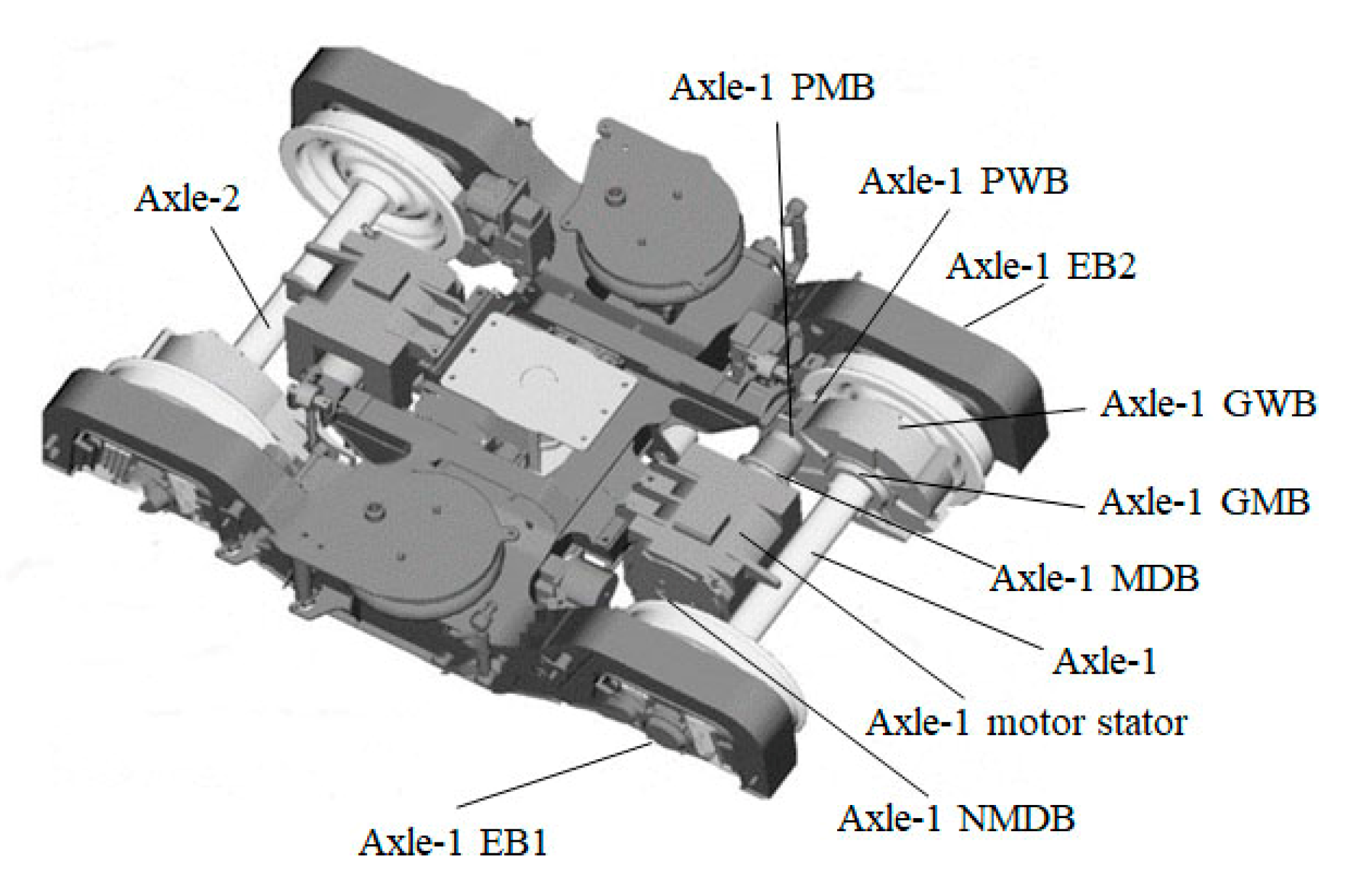
Temperature sensors were installed at a total of 36 positions, including each axle end bearing, bearing of motor side and wheel side of gearbox of a high-speed train. Take the 1st axle (Axle-1) for example. There are 9 sensors for Axle-1, the sensor of the bearing of the 1st end of the axle (Axle-1 EB1), the sensor of the bearing of the 2st end of the axle (Axle-1 EB2), the sensor of the motor drive end bearing (Axle-1 MDB), the sensor of the motor non-drive end bearing (Axle-1 NMDB), the sensor of the pinion gearbox motor side bearing (Axle-1 PMB), the sensor of the pinion gearbox wheel side bearing (Axle-1 PWB), the sensor of the large gearbox motor side bearing (Axle-1 GMB), the sensor of the large gearbox wheel side bearing (Axle-1 GWB) and the sensor of the motor stator. Each sensor had two dual-channel values and there were two symmetrical sensors collecting the values of the same object, preventing loss of data due to sensor damage. The location of the sensor is shown in Figure 1The sensor number is shown in Table 1.
2.2. Test Results
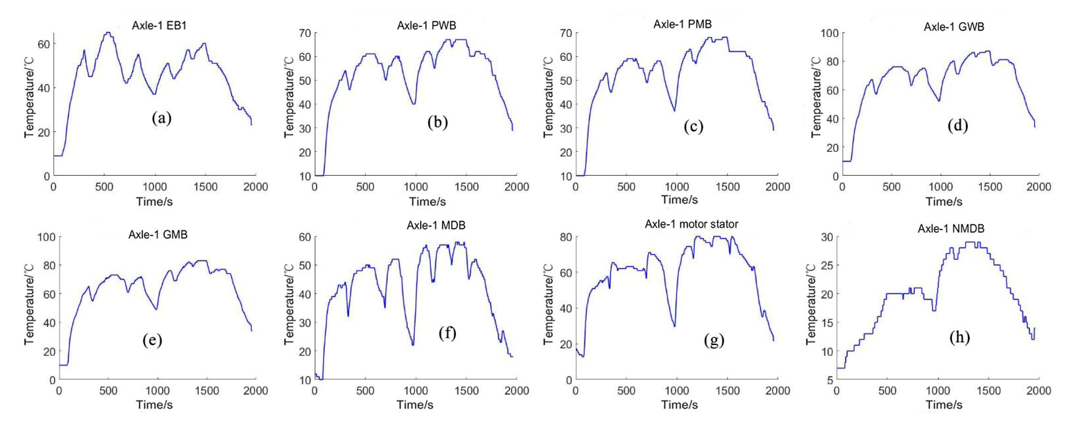
The experimental train runs on the Beijing–Shanghai high-speed railway (between Beijing and Shanghai). The cumulative daily mileage is 2650 km and the driving time is 572 min. The axle temperature data of train-2 running for 11 days were collected by the sensors arranged at the measuring points, as shown in Table 1. The acquisition frequency was 2 s once. In order to explore the variation law of axle temperature with time, temperatures of the bearing of the 1st end (EB1), the bearing of the pinion gearbox motor side (PMB), the bearing of the pinion gearbox wheel side (PWB), the bearing of the great gearbox motor side (GMB), the bearing of the great gearbox wheel side (GWB), the bearing of the motor drive end, the bearing of the motor non-driving end and the bearing of the motor stator on axle-1 were processed as typical data. The curves of temperature changes with time are shown in Figure 2.
As can be seen from the above figures, the axle temperature at each position varies with time, showing different trends and relationships. Near the end of power output, such as motor stator and the end of traction motor drive, the temperature change is relatively drastic with a large range; however, when gradually moving away from the end of power output, such as from the motor drive end to the gear box, the change in axle temperature slows down and its amplitude decreases. There is significant fluctuation of axle temperature at each position, showing strong nonlinear characteristics.
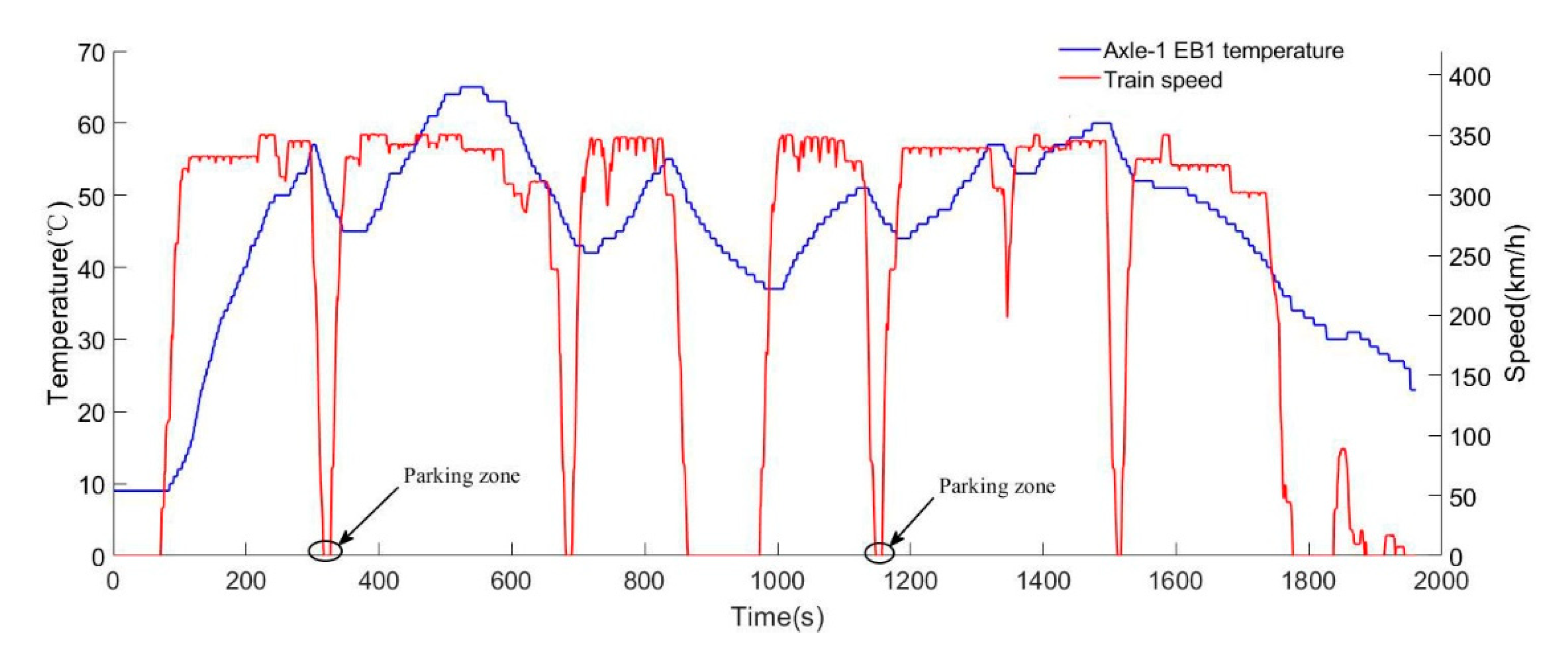
The change in axle temperature was related to the running characteristics of the train. Here, the temperature change of the bearing of the 1st end of axle-1 (Axle-1 EB1) was compared with the train running speed, as shown in Figure 3. The correlation between the temperature change of the bearing and the train speed is apparent. The axle temperature has the same variation trend with the fluctuation of the train speed, with a little lag in time. However, the change in axle temperature not only depends on the change in speed but also is subjected to other driving characteristics.
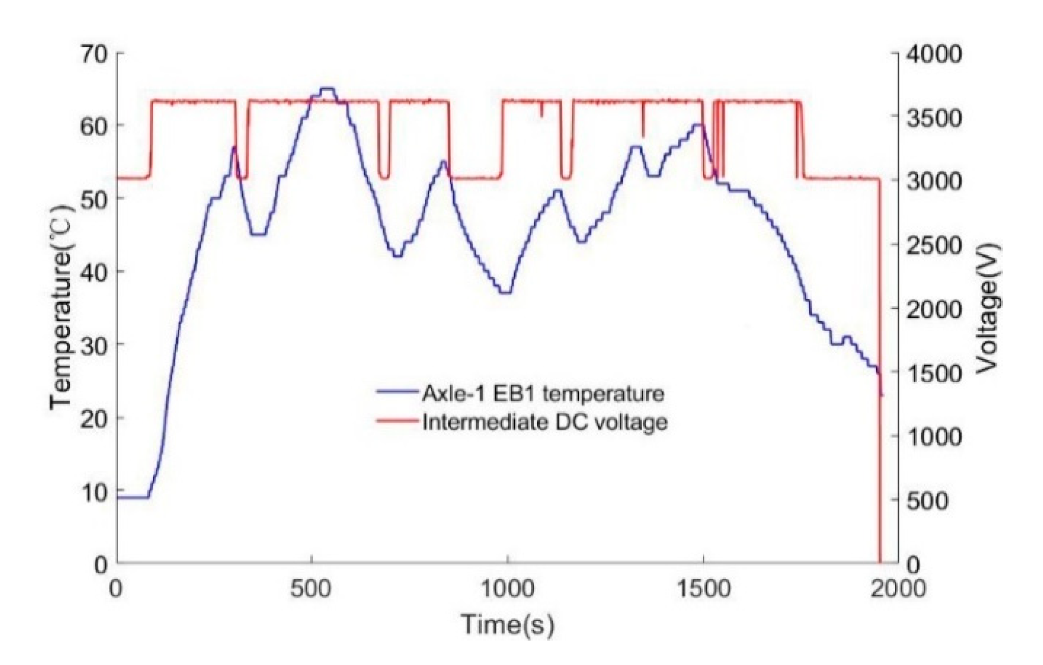
As shown in Figure 4, the axle temperature variation presents a certain correlation with DC voltage, and the correspondence is more complicated. Therefore, to accurately predict the change in axle temperature, multiple driving characteristics should be considered simultaneously. The modeling is relatively complex. Moreover, unmeasured factors, such as collision between locomotive and track, friction and so on, also have an influence on axle temperature. There are inevitable systematic errors in the modeling with only the driving characteristics considered.
Therefore, for axle temperature prediction of each position, only the axle temperature data themselves are considered for prediction. Through neural network modeling and training, axle temperature in the future is predicted with historical data of the current prediction points by using the time-series forecasting method.
3. Neural Network Prediction
3.1. Method
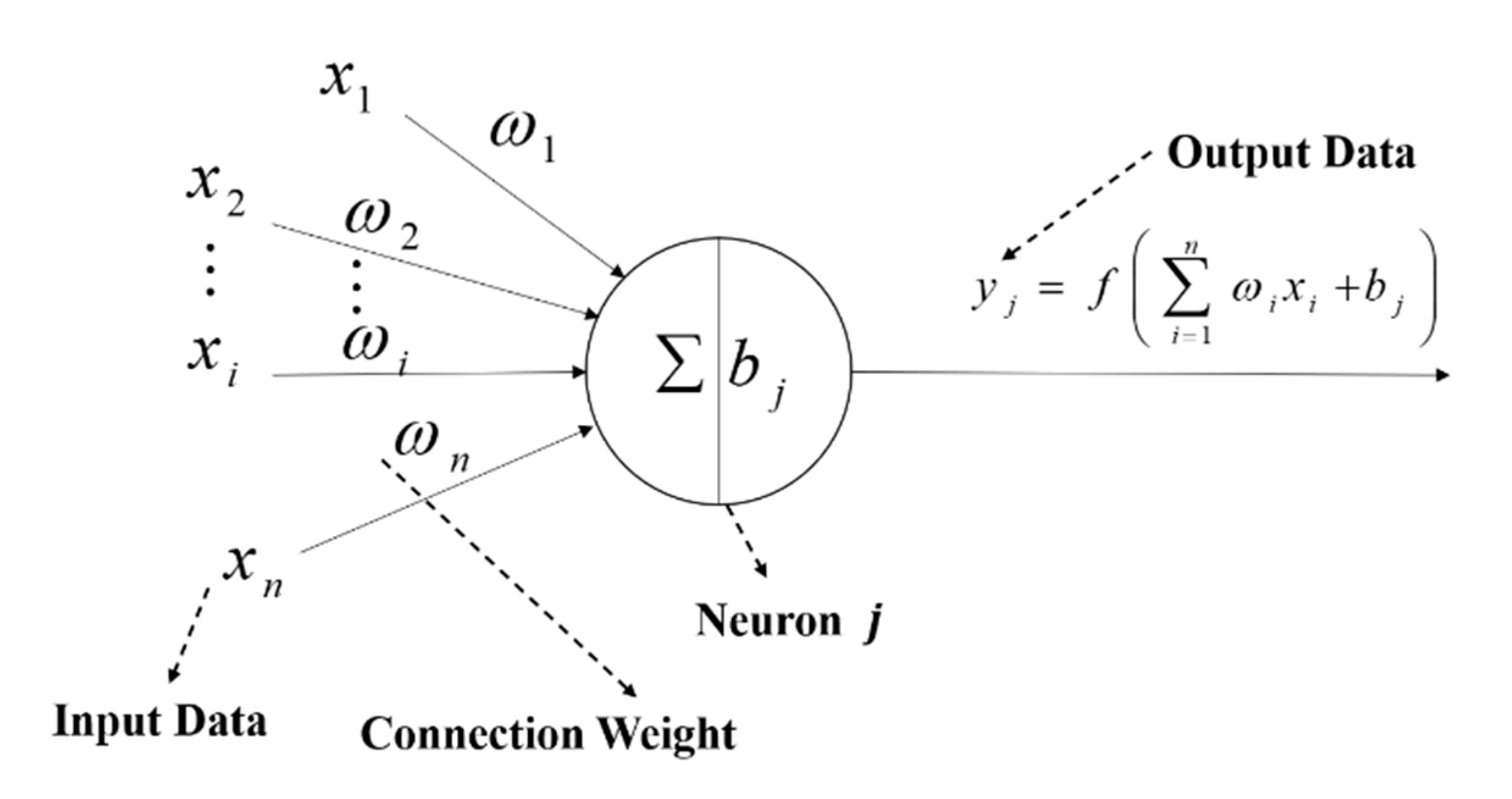
Neural networks are computational models inspired by how the human brain works. It is usually divided into several layers, and each layer contains a number of neurons. This neuron is similar to the neuron in the human brain, taking input data from several neurons in the previous layer. It multiplies the corresponding weight and sums together. Then, it adds corresponding bias of the neuron to obtain the total input of the neuron. Then, it is processed by an activation function to obtain the output data of the neuron. As shown in Figure 5, the neuron receives input data from the previous layer of neurons, multiplies the corresponding weight to calculate the sum and then adds the bias of neuron j and obtains the total input corresponding to neuron j:
Then, the output value of neuron j is:
where f is the activation function, introducing nonlinear factors into the entire neural network system. All neurons are processed in this way and passed backwards, obtaining the final output. Finally, the information transfer process is finished. Common activation functions include Sigmoid function, Relu function, Tanh function, etc. For example, the Sigmoid function takes the form of:
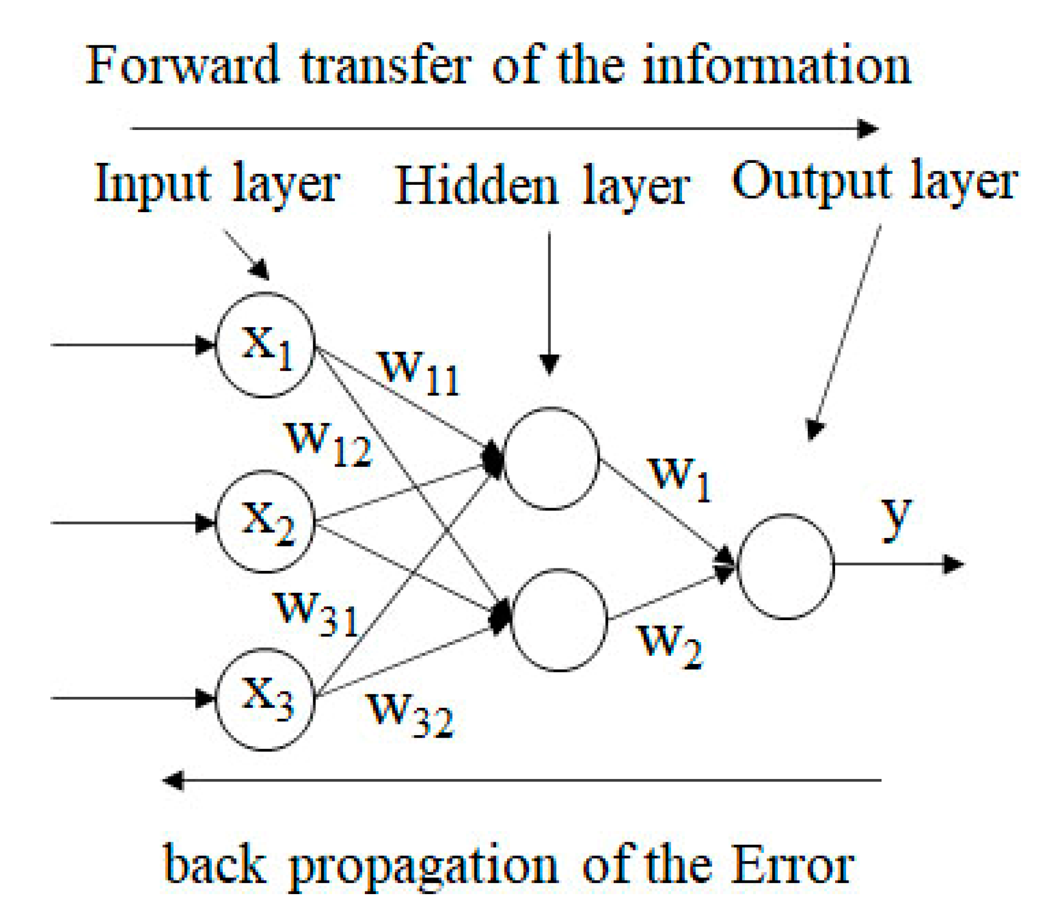
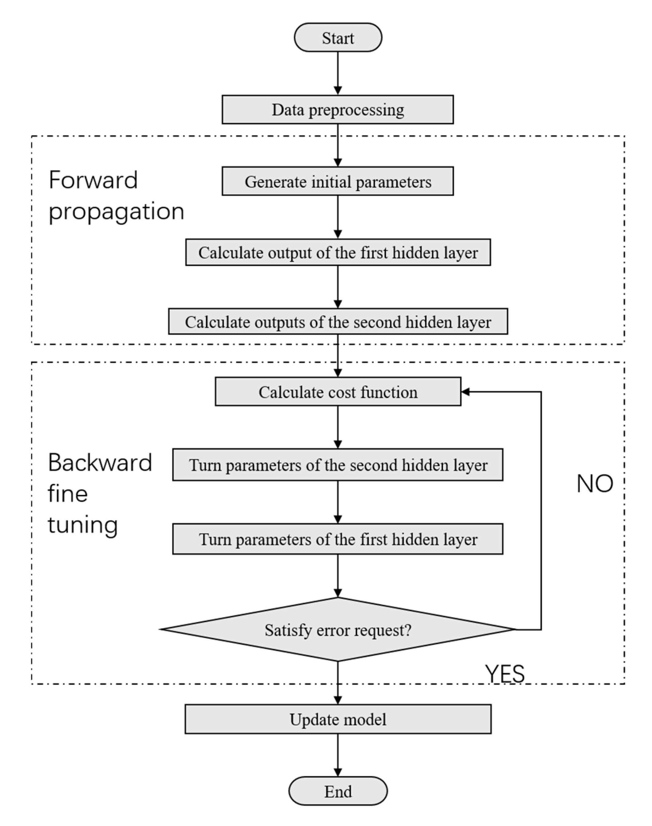
The BP neural network is a widely used neural network which consists of the input layer, the hidden layer and the output layer. The hidden layer may contain multiple layers of neurons. BP neural network, as Figure 6 shows, includes the forward transmission of data and the back propagation of errors. Firstly, the data are transmitted layer by layer from the input layer to the output layer through each neuron. After passing to the output layer, the error of the output layer can be obtained according to the output data and the target data. Then, through the back propagation of the error, the minimum value of the cost function is regarded as the goal, in combination with the gradient descent method. The connection weight of each neuron and the corresponding bias of each neuron are gradually adjusted, iterating continuously until the error reaches the set accuracy. At this time, the final weight and bias can be obtained, and the training of the model is completed.
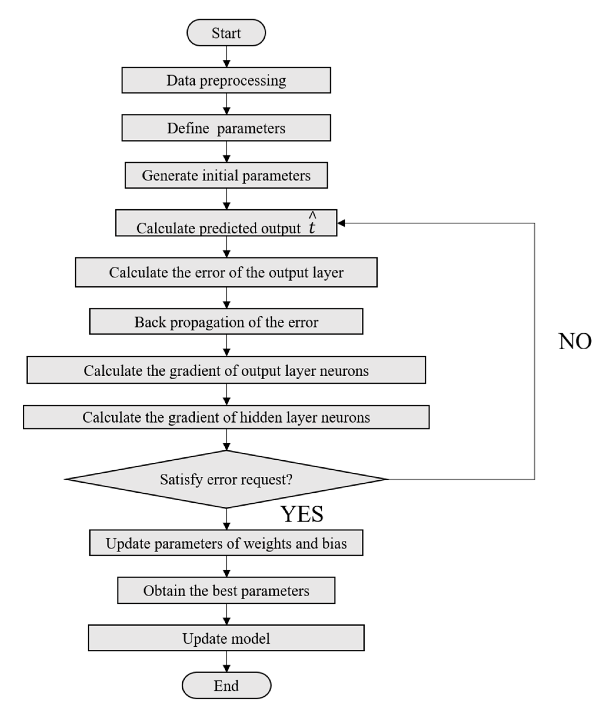
The back propagation (BP) neural network uses a typical supervised learning method. The flow chart of the BP neural network is shown in Figure 7. The mean-squared error (MSE) is defined as follows:
where E is the error between the predicted output and the actual output, is the predicted output and tj is the actual output.
The weights and biases of neural networks are updated iteratively by the gradient descent algorithm, as follows:
where v represents parameters of weights and biases, and Δv represents the gradient of weights and biases.
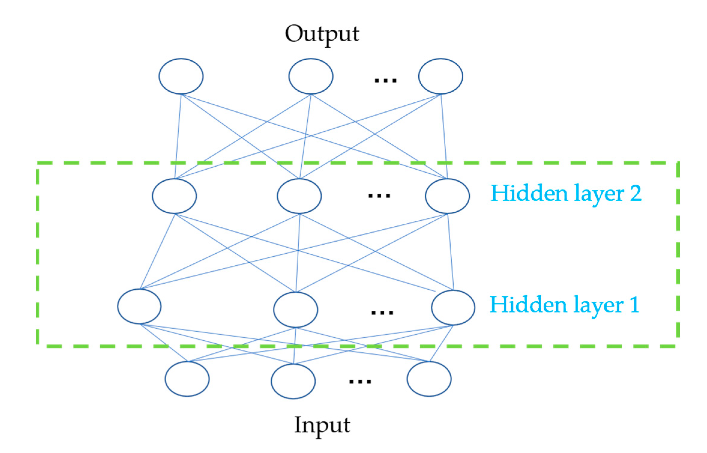
According to the number of hidden layers, neural networks are divided into single hidden layer neural networks and multi-hidden layer neural networks. The multi-hidden layer neural network is a kind of deep learning structure. Deep learning models obtain the ability to process abstract concepts by simulating the complex cognitive laws of the human brain by increasing the number of layers in the network. The multi-hidden layer neural network theoretically has the ability to approximate any nonlinear continuous mapping, so it is very suitable for the modeling and control of nonlinear systems and is currently used more in the industrial field. The double hidden layer BP neural network, shown in Figure 8, has good generalization ability, and the nonlinear approximation effect is good.
Using the trained model, after inputting the input data, the predicted value of the sample can be calculated by the neural network. With the increasing size and complexity of data, neuroevolution is used to optimize the strengths of neural connections and the structure of the network, such as conventional neuro evolution (CNE) [17] and differential evolution for neural networks (DENN) [18]. Moreover, some scholars have combined neural networks with data feature extraction technology to improve the fault recognition ability [19,20].
3.2. Data Input
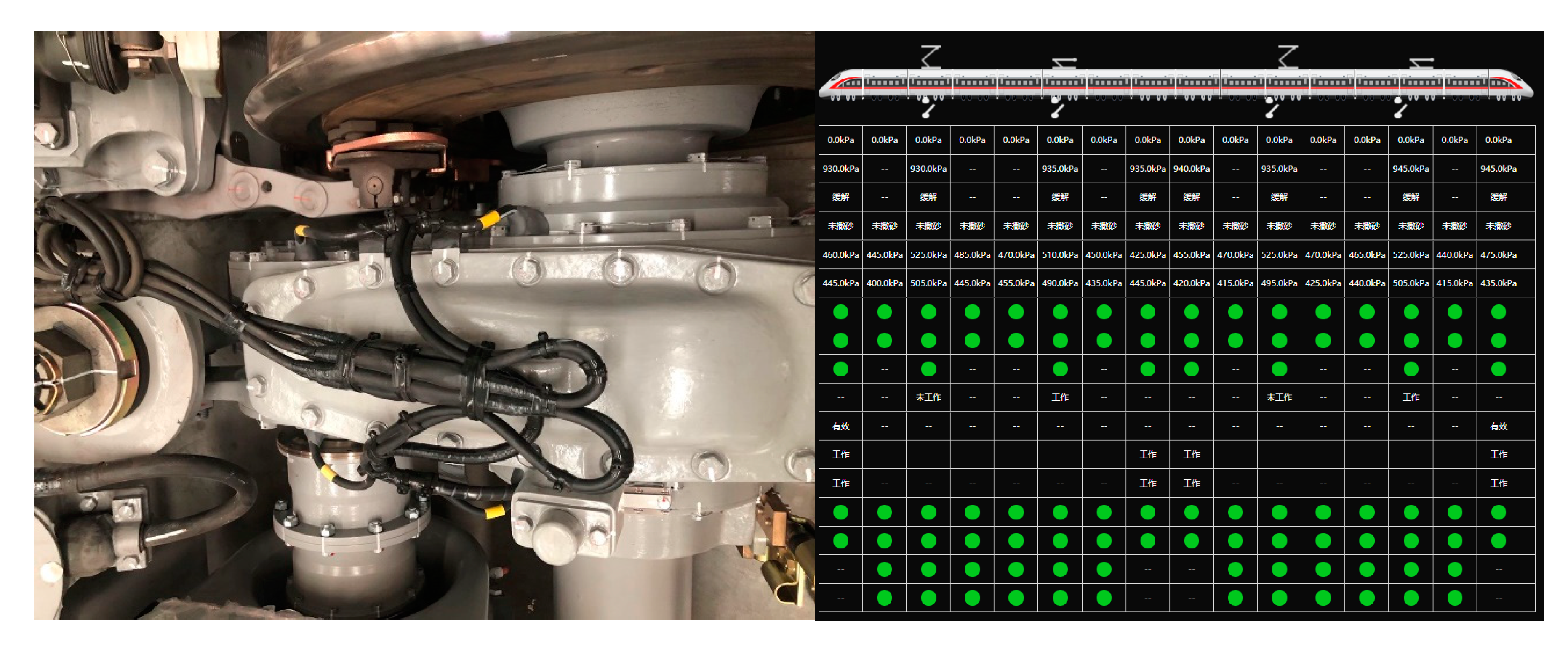
First of all, 11 days of sample data were pooled for maximum down sampling. One of the largest pieces of data was selected in every 10 data intervals. Since the sensor sampling time interval before sampling was 2 s, the time interval after sampling was 20 s, and there were 40,592 samples. In this paper, all the axle temperature sensors were installed as in the left side of Figure 9, and the result of axle temperature monitoring is shown in the right side of Figure 9.
Then, according to the temperature data of a certain position to be predicted, the first temperature data of a certain time point were used to predict the temperature of nt data points after the point; this means that n = nt + 9. The interval of n data used for prediction was nk. From the current time point, one data point was taken from every nk data point in the reverse time direction for prediction until n data points were taken, , where represented the largest integer not exceeding .
For each data point of the temperature series, data points were taken as a group of input data in the reverse direction of time. One datum was taken as the output data from data points along the time direction. A sample corresponding to the point was obtained by processing the temperature series in turn, and the final sample data set was obtained.
4. Model Training and Result Analysis
4.1. Model Training
The samples of the first 10 days were taken as training data, and 100 samples were randomly selected from the 11th day as test data. In order to improve the prediction accuracy of the model, this paper compared the influence of the number of hidden layers and the number of hidden layer nodes on the prediction results. Through a large number of experiments, the optimal network model structure of the algorithm was obtained. The training model adopted a three-layer BP neural network model, in which there were two hidden layers, shown in Figure 10. The number of neurons in the first hidden layer was 20. In the second hidden layer, there were two. The maximum number of iterations was set as 1000. The iteration termination error accuracy was 1 × 10⁻⁴, and the learning rate was set to 0.02.
4.2. Prediction versus Reality
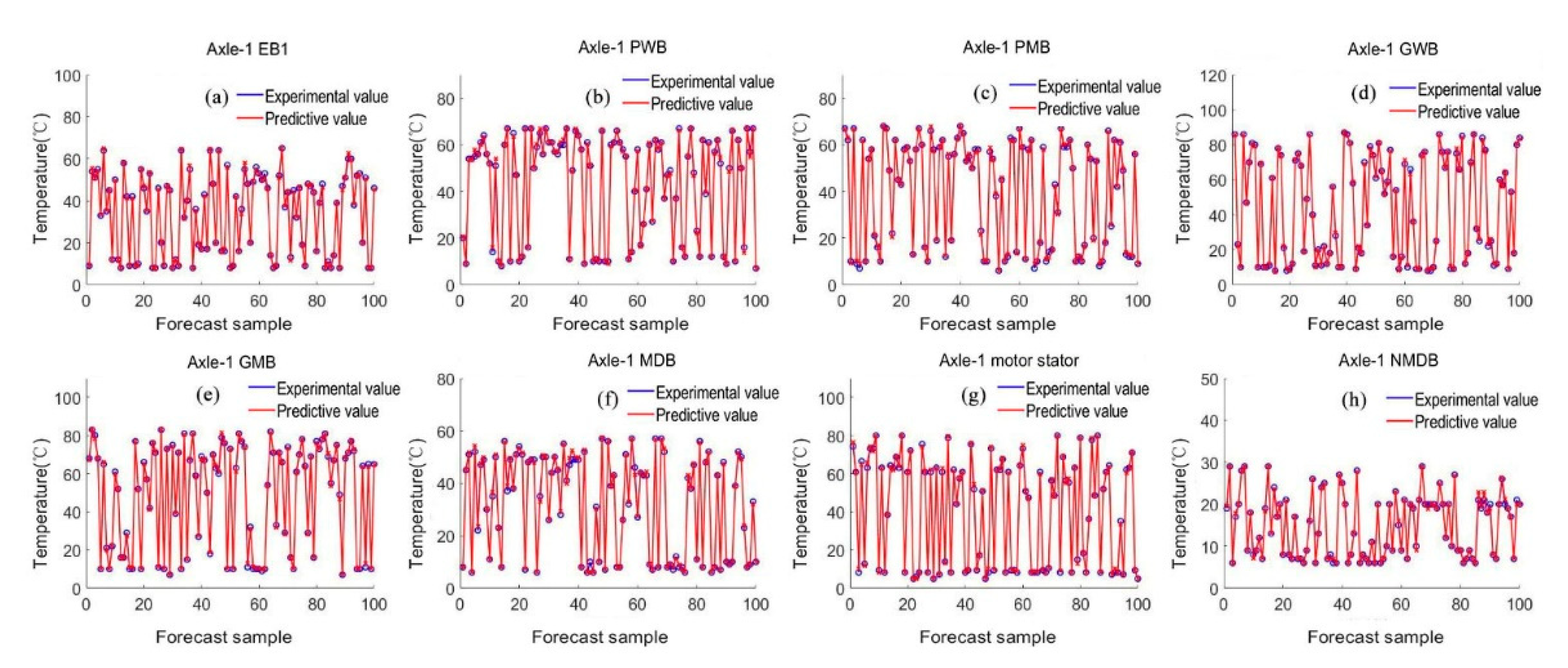
After the training, the model was used to randomly select 100 sample data at each location for axle temperature prediction. The predicted values were compared with the actual measured axle temperature value. Figure 11 shows the prediction results of axle temperature at each typical position with 3 min in advance.
It can be seen that the method can accurately predict the axle temperature of each position after 3 min. RMSE (root mean square error) and MAPE (mean absolute percentage error) are used as indicators to measure the quality of prediction results, which are defined as:
where N is the number of test samples; is the experimental value and is the predicted value. RMSE and MAPE of each predicted location on axle-1 were calculated as shown in Table 2. It can be seen that the prediction error of each position is small, and the average absolute percentage error is within 3%.
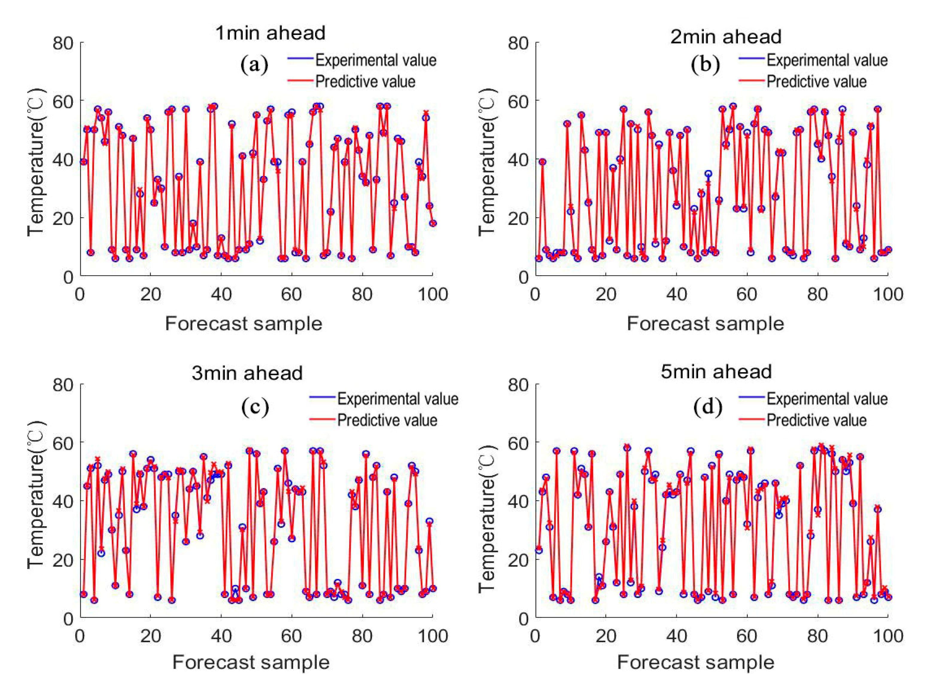
The method was used to predict the temperature of the bearing at the motor driving end of axle-1 (MDB) after 1 min, 2 min, 3 min and 5 min, respectively. It can be seen from Figure 12 that the method can maintain high accuracy even with the prediction 5 min in advance.
The RMSE and MAPE predicted by different lead times are shown in Table 3. RMSE and MAPE of prediction results increase with the extension of prediction time; in practical application, the prediction time can be selected according to the required prediction accuracy.
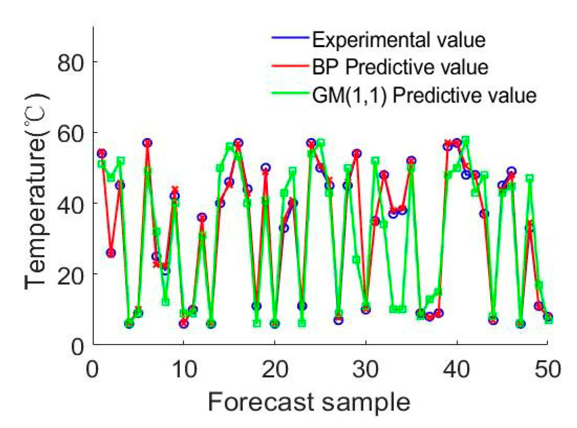
A BP neural network and gray GM (1,1) model were used to predict axle temperature 3 min in advance; the comparison of its prediction results is shown in Figure 13. It can be seen that the errors of the gray model at individual points are very large, while the prediction errors of the BP network at each point are small.
As shown in Table 4, the RMSE of the gray model is close to 10, while the average absolute percentage error reaches over 24%. It is difficult to meet the requirements of practical engineering application; however, the RMSE predicted by the BP neural network is within 1 and the MAPE is within 3%, which can provide a more accurate prediction value of axle temperature.
5. Conclusions
By means of temperature sensors at the corresponding positions of a high-speed train, axle temperature information under operation was monitored. The axle temperature and other related data were collected for 11 days. A neural network model was built, and the collected data were divided into training data and test data. The neural network model was trained with the training data. The prediction performance of the neural network prediction method was verified on the test data.
(1) By analyzing the typical position axle temperature data collected by the temperature sensors, it was found that the axle temperature near the power output end changed drastically. When moving away from the power output end, the change in axle temperature slows down; axle temperature has an apparent correlation with driving characteristics such as the train speed and the intermediate DC voltage.
(2) Combined with the neural network, a method of predicting the axle temperature of the high-speed train in advance is presented. It is verified that this method can realize the prediction accurately. The average mean absolute percentage error of axle temperature prediction in each typical position 3 min in advance is within 3%, and the RMSE error is within 1.
(3) The accuracy of different prediction times was given, which can be used as a basis for selecting prediction time in practical applications, and it can be seen that, when the forecast time is 5 min ahead, the prediction model still has high accuracy, as the MAPE is 3.3790%.
(4) Compared with the traditional gray model, the prediction accuracy of the neural network is higher. It is more suitable for predicting temperature in engineering.
Author Contributions
Conceptualization, W.H.; data curation, W.H.; formal analysis, W.H.; investigation, W.H.; methodology, W.H.; software, W.H.; supervision, F.L.; validation, W.H.; writing—original draft, W.H.; writing—review and editing, F.L. All authors have read and agreed to the published version of the manuscript.
Funding
This research was supported by the National Key R&D Plan of China (grant number 2019YFB1405202).
Conflicts of Interest
The authors declare no conflict of interest.
References
- Wang, Y.; Wu, Z.R. A Train Hot Bearing Detection System Based on Infrared Array Sensor. Appl. Mech. Mater. 2013, 672–676. [Google Scholar] [CrossRef] [Green Version]
- Ha, D.; Wang, Q.; Jiang, T.; Zhang, Y.W. Application of New Axle Temperature Monitoring System on High-Speed EMUs. J. Dalian Jiaotong Univ. 2013, 34, 89–94. (In Chinese) [Google Scholar]
- Hao, W.; Liu, F. Imbalanced Data Fault Diagnosis Based on an Evolutionary Online Sequential Extreme Learning Machine. Symmetry 2020, 12, 1204. [Google Scholar] [CrossRef]
- Xin-Zhi, C.; Kun, W. High Speed Train Axle Temperature Monitoring System Based on nRF905. Nucl. Electron.Detect. Technol. 2010, 30, 1387–1390. (In Chinese) [Google Scholar]
- Zhao, Y.; Huang, R. Metro Vehicle Axle Temperature Monitoring Device Based on Piezoelectric Vibration. Int. J. Transp. Eng. Technol. 2019, 5, 88. [Google Scholar] [CrossRef]
- Xiao-bo, A. Axle Temperature Analysis of 120 km/h Freight Trains and Prediction of Hotbox. Roll. Stock 2008, 46, 33–37. [Google Scholar]
- Xie, G.; Wang, Z.X.; Hei, X.H.; Takahashi, S.; Mochizuki, H. Axle temperature threshold prediction model of high-speed train for hot axle fault. J. Traffic Transp. Eng. 2018, 3, 129–137. [Google Scholar]
- Yu-gan, C.H.I. Analysis of Predicting the Regular Patterns of Hot Box and Axle Temperatures of Vehicles in Operation. Roll. Stock 2007, 7, 11. [Google Scholar]
- Lei, Z. Research on the Axle Temperature Changing Pattern of 120 km/h Freight Trains. Roll. Stock 2009, 47, 28–31. [Google Scholar]
- Shengjun, H. Discussion about Improvement of Prediction Quality in Hot Axle Detection. Roll. Stock 2000, 38, 37–39. [Google Scholar]
- Yin-Dong, C. Passenger Car Axle Temperature Prediction Algorithm Based on Metabolic GM (1,1) Model. Railw. Locomot. Car 2011, 31, 49–52. [Google Scholar]
- Xie, G.; Wang, Z.; Hei, X.; Takahashi, S.; Nakamura, H. Data-Based Axle Temperature Prediction of High Speed Train by Multiple Regression Analysis. In Proceedings of the 2016 12th International Conference on Computational Intelligence and Security (CIS), Wuxi, China, 16–19 December 2016; pp. 349–353. [Google Scholar]
- Ma, W.; Tan, S.; Hei, X.; Zhao, J.; Xie, G. A Prediction Method Based on Stepwise Regression Analysis for Train Axle Temperature. In Proceedings of the 2016 12th International Conference on Computational Intelligence and Security (CIS), Wuxi, China, 16–19 December 2016; pp. 386–390. [Google Scholar]
- Luo, C.; Yang, D.; Huang, J.; Deng, Y.-D. LSTM-Based Temperature Prediction for Hot-Axles of Locomotives. ITM Web Conf. 2017, 12, 1013. [Google Scholar] [CrossRef] [Green Version]
- Huang, M.T.; Gao, X.M. Motor Front Axle Temperature Forecasting Based on Phase Space Reconstruction and BP Neural Network. Adv. Mater. Res. 2013, 823, 406–410. [Google Scholar] [CrossRef]
- Franzoni, V.; Milani, A. Heuristic semantic walk for concept chaining in collaborative networks. Int. J. Web Inf. Syst. 2014, 10, 85–103. [Google Scholar] [CrossRef]
- Floreano, D.; Dürr, P.; Mattiussi, C. Neuroevolution: From architectures to learning. Evol. Intell. 2008, 1, 47–62. [Google Scholar] [CrossRef]
- Baioletti, M.; Di Bari, G.; Poggioni, V. Differential Evolution for Neural Networks Optimization. Mathematics 2020, 8, 69. [Google Scholar] [CrossRef] [Green Version]
- Glowacz, A. Fault diagnostics of acoustic signals of loaded synchronous motor using SMOFS-25-EXPANDED and selected classifiers. Teh. Vjesn. Tech. Gaz. 2016, 23, 1365–1372. [Google Scholar] [CrossRef] [Green Version]
- Glowacz, A. Recognition of Acoustic Signals of Synchronous Motors with the Use of MoFS and Selected Classifiers. Meas. Sci. Rev. 2015, 15, 167–175. [Google Scholar] [CrossRef] [Green Version]
Figure 1.
Schematic diagram of sensor layout.

Figure 2.
(a–h) Typical position axle temperature changes with time: (a) Typical position axle temperature changes with time for Axle-1 EB1, (b) Typical position axle temperature changes with time for Axle-1 PWB, (c) Typical position axle temperature changes with time for Axle-1 PMB, (d) Typical position axle temperature changes with time for Axle-1 GWB, (e) Typical position axle temperature changes with time for Axle-1 GMB, (f) Typical position axle temperature changes with time for Axle-1 MDB, (g) Typical position axle temperature changes with time for Axle-1 motor stator, and (h) Typical position axle temperature changes with time for Axle-1 NMDB.

Figure 3.
Correlation between axle temperature change and train speed.

Figure 4.
Correlation between axle temperature change and voltage.

Figure 5.
Schematic diagram of neurons.

Figure 6.
Schematic diagram of neural network data transfer.

Figure 7.
Flowchart of the BP neural network.

Figure 8.
Structure of the double hidden layer BP network model.

Figure 9.
Axle temperature sensors and monitoring.

Figure 10.
Flowchart of the proposed model.

Figure 11.
(a–h) Comparison of predicted and experimental axle temperature: (a) Comparison of predicted and experimental axle temperature for Axle-1 EB1, (b) Comparison of predicted and experimental axle temperature for Axle-1 PWB, (c) Comparison of predicted and experimental axle temperature for Axle-1 PMB, (d) Comparison of predicted and experimental axle temperature for Axle-1 GWB, (e) Comparison of predicted and experimental axle temperature for Axle-1 GMB. (f) Comparison of predicted and experimental axle temperature for Axle-1 MDB, (g) Comparison of predicted and experimental axle temperature for Axle-1 motor stator, and (h) Comparison of predicted and experimental axle temperature for Axle-1 NMDB.

Figure 12.
(a–d) Comparison of prediction accuracy of different lead times: (a) 1 min ahead; (b) 2 min ahead; (c) 3 min ahead; (d) 5 min ahead.
Figure 12.
(a–d) Comparison of prediction accuracy of different lead times: (a) 1 min ahead; (b) 2 min ahead; (c) 3 min ahead; (d) 5 min ahead.

Figure 13.
Comparison of prediction accuracy between the BP neural network and the GM (1,1) model.


Table 1.
Temperature sensor location.
| Sensor Number | Sensor Location | Sensor Number | Sensor Location |
|---|---|---|---|
| 1~8 | Bearing of two end of axle-1/2/3/4 | 21~24 | axle-1/axle-2/axle-3/axle-4 motor stator |
| 9~12 | axle-1/axle-2/axle-3/axle-4 Pinion gearbox motor side bearing (PMB) | 25~28 | axle-1/axle-2/axle-3/axle-4 motor non-drive end bearing (NMDB) |
| 13~16 | axle-1/axle-2/axle-3/axle-4 Pinion gearbox wheel side bearing (PWB) | 29~32 | axle-1/axle-2/axle-3/axle-4 -large gearbox motor side bearing (GMB) |
| 17~20 | axle-1/axle-2/axle-3/axle-4 motor drive end bearing (MDB) | 33~36 | axle-1/axle-2/axle-3/axle-4 large gearbox wheel side bearing (GWB) |
Table 2.
RMSE and MAPE for each predicted position.
| Predicted Location | RMSE | MAPE | Predicted Location | RMSE | MAPE |
|---|---|---|---|---|---|
| Axle-1 EB1 | 0.7858 | 1.5609% | GMB | 0.8198 | 1.8473% |
| PWB | 0.8519 | 1.4176% | MDB | 0.9455 | 2.2800% |
| PMB | 0.7708 | 2.6951% | Motor stator | 0.9162 | 2.6949% |
| GWB | 0.8203 | 2.3608% | NMDB | 0.4569 | 1.6366% |
Table 3.
Comparison of forecast errors of different times in advance of MDB.
| Advance Time | RMSE | MAPE |
|---|---|---|
| 1 min | 0.6080 | 1.2593% |
| 2 min | 0.7965 | 2.2658% |
| 3 min | 0.9455 | 2.2800% |
| 5 min | 1.0302 | 3.3790% |
Table 4.
Comparison of prediction error between BP neural network and GM (1,1) model.
| Method of Prediction | RMSE | MAPE |
|---|---|---|
| BP neural network | 0.9446 | 2.4416% |
| GM (1,1) | 9.9448 | 24.2271% |
© 2020 by the authors. Licensee MDPI, Basel, Switzerland. This article is an open access article distributed under the terms and conditions of the Creative Commons Attribution (CC BY) license (http://creativecommons.org/licenses/by/4.0/).
Share and Cite
MDPI and ACS Style
Hao, W.; Liu, F. Axle Temperature Monitoring and Neural Network Prediction Analysis for High-Speed Train under Operation. Symmetry 2020, 12, 1662. https://0-doi-org.brum.beds.ac.uk/10.3390/sym12101662
AMA Style
Hao W, Liu F. Axle Temperature Monitoring and Neural Network Prediction Analysis for High-Speed Train under Operation. Symmetry. 2020; 12(10):1662. https://0-doi-org.brum.beds.ac.uk/10.3390/sym12101662
Chicago/Turabian StyleHao, Wei, and Feng Liu. 2020. "Axle Temperature Monitoring and Neural Network Prediction Analysis for High-Speed Train under Operation" Symmetry 12, no. 10: 1662. https://0-doi-org.brum.beds.ac.uk/10.3390/sym12101662
Note that from the first issue of 2016, this journal uses article numbers instead of page numbers. See further details here.