Dynamics Analysis and Synchronous Control of Fractional-Order Entanglement Symmetrical Chaotic Systems

Abstract

In this paper, the Adomian decomposition method (ADM) semi-analytical solution algorithm is applied to solve a fractional-order entanglement symmetrical chaotic system. The dynamics of the system are analyzed by the Lyapunov exponent spectrum, bifurcation diagrams, poincaré diagrams, and chaos diagrams. The results show that the systems have rich dynamics. Meanwhile, sliding mode synchronizations of fractional-order chaotic systems are investigated theoretically and numerically. The results show the effectiveness of the proposed method and potential application value of fractional-order systems.

1. Introduction

The concept of fractional-order calculus can be traced back to a letter written by L’Hospital to Leiniz in 1695, which mentioned how to solve when the order is 0.5 and how to understand a differential equation with arbitrary order. Fractional-order calculus development is slow because there is no practical physics and engineering application background. Recently, it has been found that fractional calculus operators are widely used in nature, electromagnetic oscillation, mechanics of materials and other scientific and technological fields. At the same time, fractional wavelet transform, fractional Fourier transform and fractional image processing have been given attention by researchers in the field of signal processing [1,2,3,4,5]. Fractional order is an extension of integer order, and the dynamic behavior of the system is not only related to the parameters of the system itself, but also to fractional order operators. With the addition of fractional operators, the complexity of the system and the maximum Lyapunov exponent become larger; that is, the dynamic behavior of the fractional system becomes more complex, which makes the fractional chaotic system have wide application values in the fields of radio and information security. Regarding combining fractional order systems with nonlinear chaotic systems, many scholars have proposed many fractional order chaotic systems, such as fractional-order Lorenz chaotic or hyperchaotic systems [6], fractional-order chaotic systems with line equilibrium [7], and so on [8,9,10].

Particularly, we need to find a numerical solution method for fractional-order chaotic systems. At present, scholars have made fruitful achievements in fractional system analysis, control and application. Regarding fractional chaotic system analysis, scholars have obtained some achievements based on the frequency-domain method (FDM) [11], the Adomian decomposition method (ADM) [5,6,7,9], and the Adams–Bashforth–Moulton (ABM) algorithm [12,13,14]. ABM is a classical numerical simulation algorithm for fractional systems, but it takes a long time to simulate and wastes significant computer resources. At the same time, it is difficult to calculate the Lyapunov exponent of the system because of the accumulated historical data. ADM has smaller error than ABM in finite term expression, wastes less computer resources and has a faster calculation speed. In essence, FDM uses high-order systems to simulate fractional-order systems, but there are large errors in both high-frequency and low-frequency bands [15]. Ref. [16] illustrates that fractional chaotic systems are more complex than integer chaotic systems in terms of system complexity and maximum Lyapunov exponent. When the system order is smaller, the system is more complicated [9,16,17], However, most researchers use the ADM method to simulate fractional chaotic systems with product nonlinear terms, but no one has studied those with special functions. The main reason is that special functions make Adomian decomposition method more complex.

On the other hand, hot research on chaotic systems mainly focuses on chaos control and synchronization [18,19,20,21,22,23,24,25,26,27,28,29,30,31]. Chaos synchronization posits that the initial states of two systems with the same structure or different structures are different, but after a period of time, the systems are synchronized through the adjustment of the controller. There are many types of chaotic synchronization, including complete synchronization [18,19,20,21,22,23,24,25,26,27,28,29], projective synchronization [18,19], anti-synchronization [20], quasi-synchronisation [21], generalized synchronization [22,24,25] and so on. Meanwhile, various synchronization methods, such as linear and nonlinear feedback control [30,31], active control [32], and sliding-modle control [33], have been successfully used for synchronizing chaotic or fractional-order chaotic systems [34,35].

The rest of the present paper is organized as follows. In Section 2, the fractional-order entanglement systems are presented, and the solution of this system is derived based on the ADM algorithm. In Section 3, the bifurcation diagram, phase diagrams and Lyapunov exponents spectrum are employed to analyze the dynamics of the system. In Section 4, the adaptive sliding mode controllers are designed to realize synchronous control, and numerical simulations demonstrate the feasibility of synchronization analysis. Finally, the obtained results are summarized in Section 5.

2. Solution of Fractional Chaotic System Based on Adomian Decomposition

2.1. Adomian Decomposition

Several definitions exist regarding fractional calculus, and Caputo derivation and Riemann–Liouville (R–L) intergration definitions are among the two most commonly used calculus definitions.

The fractional-order derivation of a function f(t) is defined as follows:

$${}_{}{}^{C}D{}_{t_0}^{q}f\left(t\right)=\frac{1}{\Gamma \left(1-q\right)}{{\displaystyle \int }}_{t_0}^t{(t-\tau )}^{-q}{f}^{\prime }(\tau )d\tau$$

(1)

Consider a nonlinear fractional-order differential equation ${}_{}{}^{C}D{}_{t_0}^{q}x\left(t\right)=f\left(x\left(t\right)\right)+g\left(t\right)$, where $x\left(t\right)={[x_1\left(t\right),x_2\left(t\right),\dots x_n\left(t\right)]}^T$ are state variables, and $g\left(t\right)={[g_1\left(t\right),g_2\left(t\right),\dots g_n\left(t\right)]}^T$ is the constant parts.The function f(x(t)) is written as a sum of two terms. Then, the differential equation becomes the following:

$${}^C{D}_{t_0}^{q}x(t)=Lx(t)+Nx(t)+g(t)$$

(2)

where L and N represent the linear item and nonlinear item, respectively. We set initial state $x^{\left(k\right)}\left(t_0^{+}\right)=b_k$, $k=0,\cdots m-1$.After applying the fractional integral n to both sides of Equation (6), we obtain:

$$x(t)=J_{t_0}^{q}Lx(t)+J_{t_0}^{q}Nx(t)+J_{t_0}^{q}g(t)+{\displaystyle \sum _{k=0}^{m-1}{b}_k\frac{{(t-t_0)}^k}{k!}}$$

(3)

The numerical solution is expressed is as:

$$x\left(t\right)={{\displaystyle \sum }}_{i=0}^{\infty }{x}^i=J_{t_0}^q{{\displaystyle \sum }}_{i=0}^{\infty }{x}^i+J_{t_0}^q{{\displaystyle \sum }}_{i=0}^{\infty }{A}^i+J_{t_0}^{q}g+{{\displaystyle \sum }}_{k=0}^{m-1}{b}_k\frac{{(t-t_0)}^k}{k!}$$

(4)

Based on the ADM algorithm in Ref. [16], the superscript i symbolizes the element of the decomposition series x⁰, x¹, x²,... xⁱ,..., derived from:

$$\left\{\begin{array}{l}{x}^0=J_{t_0}^{q}g+{\displaystyle \sum _{k=0}^{m-1}{b}_k\frac{{(t-t_0)}^k}{k!}}\\ x^1=J_{t_0}^{q}L{x}^0+J_{t_0}^q{A}^0(x^0)\\ x^2=J_{t_0}^{q}L{x}^1+J_{t_0}^q{A}^1(x^0,x^1)\\ ⋮\\ x^i=J_{t_0}^{q}L{x}^{i-1}+J_{t_0}^q{A}^{i-1}(x^0,x^1\cdots x^{i-1})\\ ⋮\end{array}\right.$$

(5)

2.2. Fractional-Order Entanglement Chaotic Systems

A class of linear system models are as follows:

$$\left\{\begin{array}{l}\dot{x}=by-ax\\ \dot{y}=-ba-cy\end{array}\right..$$

(6)

Another linear system model is as follows:

$$\dot{z}=-dz.$$

(7)

Based on Ref. [36], if the above two systems are entangled, a new class of chaotic entangled systems can be obtained. The dynamic equation is as follows:

$$\left\{\begin{array}{l}\dot{x}=by-ax+h\sin z\\ \dot{y}=-bx-cy+h\sin x\\ \dot{z}=-dz+h\sin y\end{array}\right.$$

(8)

System (8) can generate complex chaotic attractors, and it has three typical parameter sets. Change the above system equations to the following fractional-order form:

$$\left\{\begin{array}{l}\frac{d{x}^{q_1}}{d^{q_1}t}=by-ax+h\sin z\\ \frac{d{y}^{q_1}}{d^{q_1}t}=-cy-bx+h\sin x\\ \frac{d{z}^{q_1}}{d^{q_1}t}=-dz+h\sin y\end{array}\right.$$

(9)

where x, y, z are state variables, a, b, c, h are system (9) parameters, (sin3z, cosx, siny) is an entangled term, and q1 is the fractional order. Entanglement terms are represented by bounded nonlinear functions [36], which are functions of states x, y, z, y and z. The nonlinear part of the system is not a simple product term, but is realized by a more complex trigonometric function, which is more popularized and applied by compounding the practical engineering system.

$$\left\{\begin{array}{l}{\mathrm{A}}^0=\mathrm{F}(u_0)=\sin u^0\\ {\mathrm{A}}^1=u^1{\mathrm{F}}^{\prime }(u_0)=u^1\cos u^0\\ {\mathrm{A}}^2=u^2{\mathrm{F}}^{\prime }(u_0)+\frac{1}{2!}{(u^1)}^2{\mathrm{F}}^{″}(u_0)=u^2\cos u^0-\frac{1}{2}{(u^1)}^2\sin u^0\\ {\mathrm{A}}^3=u^3{\mathrm{F}}^{\prime }(u_0)+u^1{u}^2{\mathrm{F}}^{″}(u_0)+\frac{1}{3!}{(u^1)}^3{\mathrm{F}}^{‴}(u_0)\\ =u^3\cos u^0-u^1{u}^2\sin u^0-\frac{1}{6}{(u^1)}^3\cos u^0\end{array}\right.$$

(10)

The initial condition is:

$$\left\{\begin{array}{l}{x}^0=x(t_0)=c_1^0\\ y^0=y(t_0)=c_2^0\\ z^0=z(t_0)=c_3^0\end{array}\right.$$

(11)

According to domain decomposition methods [31] and fractional calculus properties, the following properties are obtained:

$$\left\{\begin{array}{l}{x}^1=(b{c}_2^0-a{c}_1^0+h\sin c_3^0)\frac{{(t-t_0)}^q}{\Gamma (q+1)}\\ y^1=(-c{c}_2^0-b{c}_1^0+h\sin c_1^0)\frac{{(t-t_0)}^q}{\Gamma (q+1)}\\ z^1=\left(-d{c}_3^0+h\sin c_2^0\right)\frac{{(t-t_0)}^q}{\Gamma (q+1)}\end{array}\right.$$

(12)

where $x^1$, $y^1$, $z^1$ is the values of systems (3), and $h_s=t-t_0$ is iteration step size. $\mathsf{\Gamma }(•)$ is the gamma function. The corresponding variables are assigned to the corresponding values; therefore, let:

$$\left\{\begin{array}{l}{c}_1^1=b{c}_2^0-a{c}_1^0+h\sin c_3^0\\ c_2^1=-c{c}_2^0-b{c}_1^0+h\sin c_1^0\\ c_3^1=-d{c}_3^0+h\sin c_2^0\end{array}\right.$$

(13)

$$\left\{\begin{array}{l}{c}_1^2=b{c}_2^1-a{c}_1^1+h{c}_3^1\cos c_3^0\\ c_2^2=-c{c}_2^1-b{c}_1^1+h{c}_1^1\cos c_1^0\\ c_3^2=-d{c}_3^1+h{c}_2^1\cos c_2^0\end{array}\right.$$

(14)

$$\left\{\begin{array}{l}{c}_1^3=b{c}_2^2-a{c}_1^2+h{c}_3^2\cos c_3^0-\frac{1}{2}h{\left(c_3^1\right)}^2\sin c_3^0\frac{\Gamma (2q+1)}{{\Gamma }^2(q+1)}\\ c_2^3=-c{c}_2^2-b{c}_1^2+h{c}_1^2\cos c_1^0-\frac{1}{2}h{\left(c_1^1\right)}^2\sin c_1^0\frac{\Gamma (2q+1)}{{\Gamma }^2(q+1)}\\ c_3^3=-d{c}_3^2+h{c}_2^2\cos c_2^0-\frac{1}{2}h{\left(c_2^1\right)}^2\sin c_2^0\frac{\Gamma (2q+1)}{{\Gamma }^2(q+1)}\end{array}\right.$$

(15)

$$\left\{\begin{array}{c}{c}_1^4=b{c}_2^3-a{c}_1^3+h{c}_3^{3}cos{c}_3^0-h{c}_3^1{c}_3^{2}sin{c}_3^0\frac{\Gamma (3q+1)}{\Gamma (q+1)\Gamma (2q+1)}-\frac{1}{6}h{\left(c_3^1\right)}^{3}cos{c}_3^0\frac{\Gamma (6q+1)}{{\Gamma }^2(3q+1)}\hfill \\ c_2^4=-c{c}_2^3-b{c}_1^3+h{c}_1^3\cos 3c_1^0-h{c}_1^1{c}_1^{2}sin{c}_1^0\frac{\Gamma (3q+1)}{\Gamma (q+1)\Gamma (2q+1)}-\frac{1}{6}h{\left(c_1^1\right)}^{3}cos{c}_1^0\frac{\Gamma (6q+1)}{{\Gamma }^2(3q+1)}\hfill \\ c_3^4=-d{c}_3^3+h{c}_2^{3}cos{c}_2^0-h{c}_2^1{c}_2^{2}sin{c}_2^0\frac{\Gamma (3q+1)}{\Gamma (q+1)\Gamma (2q+1)}-\frac{1}{6}h{\left(c_2^1\right)}^{3}cos{c}_2^0\frac{\Gamma (6q+1)}{{\Gamma }^2(3q+1)}\hfill \end{array}\right.$$

(16)

Thus, the solution of system (9) is defined as:

$$\left\{\begin{array}{c}x\left(t\right)=c_1^0+c_1^1\frac{{\left(t-t_0\right)}^q}{\Gamma (q+1)}+c_1^2\frac{{\left(t-t_0\right)}^{2q}}{\Gamma (2q+1)}+c_1^3\frac{{\left(t-t_0\right)}^{3q}}{\Gamma (3q+1)}+c_1^4\frac{{\left(t-t_0\right)}^{4q}}{\Gamma (4q+1)}\hfill \\ y\left(t\right)=c_2^0+c_2^1\frac{{\left(t-t_0\right)}^q}{\Gamma (q+1)}+c_2^2\frac{{\left(t-t_0\right)}^{2q}}{\Gamma (2q+1)}+c_2^3\frac{{\left(t-t_0\right)}^{3q}}{\Gamma (3q+1)}+c_2^4\frac{{\left(t-t_0\right)}^{4q}}{\Gamma (4q+1)}\hfill \\ z\left(t\right)=c_3^0+c_3^1\frac{{\left(t-t_0\right)}^q}{\Gamma (q+1)}+c_3^2\frac{{\left(t-t_0\right)}^{2q}}{\Gamma (2q+1)}+c_3^3\frac{{\left(t-t_0\right)}^{3q}}{\Gamma (3q+1)}+c_3^4\frac{{\left(t-t_0\right)}^{4q}}{\Gamma (4q+1)}\hfill \end{array}\right.$$

(17)

when a = 2, b = 10, c = 3, h = 18 and initial condition [x(0), y(0), z(0)] = [1, 1, 1.1]. Using MATLAB to simulate the Equation (17), the chaotic attractor is shown in Figure 1.

2.3. Symmetric Analysis

The trigonometric function and linear function in the system are symmetrical about the origin. This system (9), which is composed of a sin function and linear function, is also symmetrical about the origin; that is, it is obtained from the invariant system after (x, y, z) → (−x, −y, −z) transformation, as shown in Figure 1.

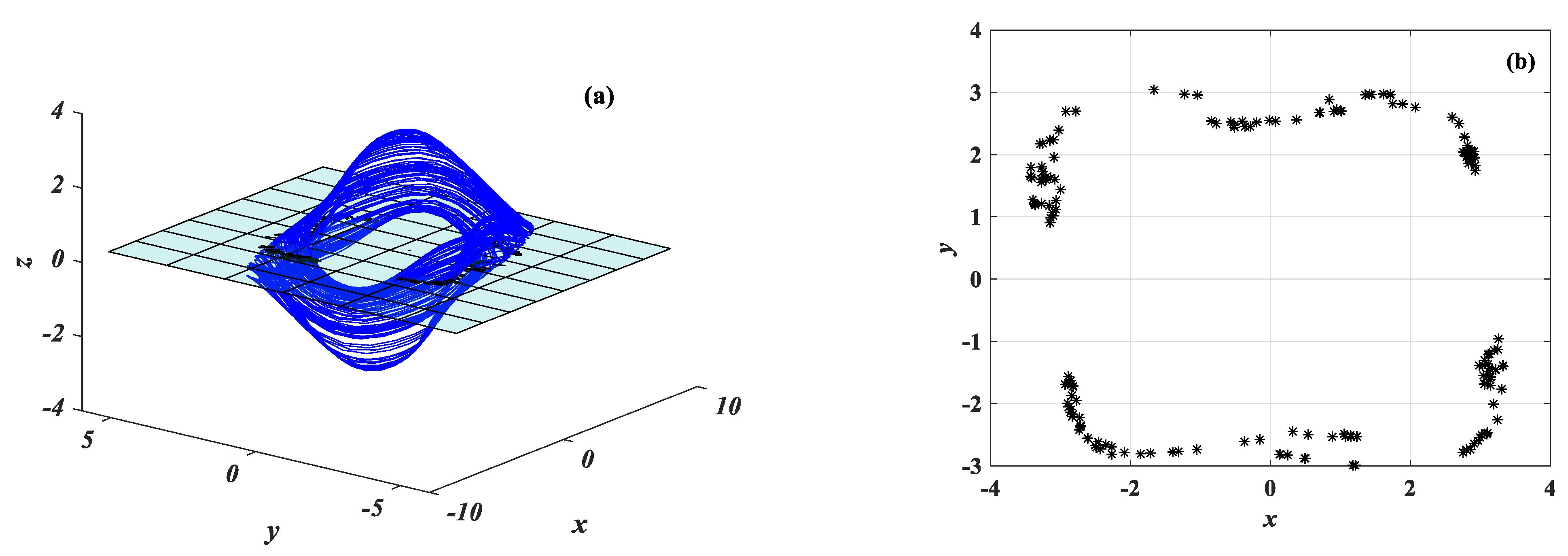
Poincaré diagrams are one of the most important tools for analyzing chaotic dynamic systems; they are applied to fractional chaotic systems to judge whether they are chaotic by observing the distribution of cut-off points. When the Poincaré diagram is filled with dense points with a fractal structure, the motion is chaotic. In this model, we take the plane z = 0, obtain the corresponding Poincaré diagrams, as shown in Figure 2, and judge system (9) to be a chaotic system.

3. Dynamics Analysis

For the dynamic analysis of the system, based on ADM, the bifurcation diagram and Lyapunov exponent are analyzed under the change of parameters. In this paper, the maximum method is used to draw the bifurcation diagram of the system, and the QR orthogonal method is used to calculate the Lyapunov exponent of the system.

3.1. Dynamics with Variations in q

Let a = 2, b = 10, c = 3, h = 18, derivative order q vary 0.8 to 1, and the initial values of state variables [x₀, y₀, z₀] = [1, 1, 0.1]. Figure 3a shows the bifurcation diagram and Lyapunov exponent spectrum with changes in system parameter q. It can be seen from the figure that under the change of derivative order q, when the bifurcation diagram of the system is in a chaotic state, the maximum Lyapunov exponent of the system is positive, and chaos and period appear when the system repeats and crosses, which is not a direct process from period to chaos. More importantly, the maximum Lyapunov exponent of the system decreases with an increase in derivative order q, and the maximum Lyapunov exponent of the system is the lowest when q = 0.81. Therefore, it is of great significance to study fractional order systems.

3.2. Dynamics with Variations in A

The fractional chaotic system (5) has three system parameters besides the fractional derivative q, and only analyzes the dynamic characteristics under the change of parameter a∈ [0, 5]. The step size of a is 0.05, q = 0.9, b = 10, c = 3, h = 18, and the initial conditions are [x0, y0, z0] = [1, 1, 1.1]. The system bifurcation diagram and Lyapunov exponent spectrum under changes are drawn by the ADM algorithm, as shown in Figure 4. The system is periodic, and other regional systems are chaotic.

To reveal the dynamics further, phase portraits of system (8) on the x-z plane with a = 0.4, a = 1.5, a = 2.3 and a = 2.8 are plotted in Figure 5a–d, respectively. These figures illustrate that the system is periodic at a = 0.4, a = 1.5 and a = 2.8, while it is chaotic at a = 2.3. In this case, from the observation that a decreases gradually, the system enters chaos through period-doubling bifurcation.

4. Synchronization Method

In this part, based on the fractional-order systems chaos synchronization method, the fractional-order systems and undisturbed system disturbed by model uncertainties and external disturbances achieve synchronization.

4.1. Synchronization Implementation

$$\left\{\begin{array}{l}\frac{d{x}_1{}^q}{d^{q}t}=b{y}_1-a{x}_1+h\sin z_1\\ \frac{d{y}_1{}^q}{d^{q}t}=-c{y}_1-b{x}_1+h\sin x_1\\ \frac{d{z}_1{}^q}{d^{q}t}=-d{z}_1+h\sin y_1\end{array}\right.$$

(18)

Suppose system (18) is disturbed by model uncertainties and external disturbances; system (18) is changed to:

$$\left\{\begin{array}{l}\frac{d{x}_1{}^q}{d^{q}t}=b{y}_1-a{x}_1+h\sin z_1\\ \frac{d{y}_1{}^q}{d^{q}t}=-c{y}_1-b{x}_1+h\sin x_1+\Delta f(y)+d(t)+u(t)\\ \frac{d{z}_1{}^q}{d^{q}t}=-d{z}_1+h\sin y_1\end{array}\right.$$

(19)

where, for the model uncertainties $\Delta f(y)$, $y={[x_1,y_1,z_1]}^{\mathrm{T}}$, and external disturbances $d(t)$, $u(t)$ are active control functions. The uncontrolled system (18) is called the disturbed fractional-order hyperchaotic system.

Then, according to error definition, the synchronization error is described as $e_1=x_1-x$, $e_2=y_1-y$, and $e_3=z_1-z$. Substitute Equation (18) to Equation (17); then, the corresponding error dynamical system can be obtained as:

$$\left\{\begin{array}{l}\frac{d{e}_1{}^q}{d^{q}t}=b{e}_2-a{e}_1+h\left(\sin z_1-\sin z\right)\\ \frac{d{e}_2{}^q}{d^{q}t}=-c{e}_2-b{e}_1+h\left(\sin x_1-\sin x\right)+\Delta f(y)+d(t)+u(t)\\ \frac{d{e}_3{}^q}{d^{q}t}=-d{e}_3+h\left(\sin y_1-\sin y\right)\end{array}\right.$$

(20)

Hypothesis 1 (H1).

$\left|\Delta f(y)\right|\le m,$and $\left|d(t)\right|\le n$, where$m,n>0$is an unknown positive constant parameter.

Lemma 1.

Ref. [37]. If $x(t)$ is a continuously differentiable function, and arbitrarily, $t\ge 0$, then

$$\frac{1}{2}{\mathrm{D}}_t{}^{\alpha }{x}^T(t)x(t)\le x^T(t){\mathrm{D}}_t{}^{\alpha }x(t),\forall \alpha \in (0,1){.}^{}$$

(21)

Lemma 2.

Ref. [37]. Fractional monotonicity principle: if $D_t{}^{\alpha }y(t)\le 0$, then $y(t)$ is monotonically decreasing at $[0,+\infty )$. If $D_t{}^{\alpha }y(t)\ge 0$, then $y(t)$ is monotonically increasing at $[0,+\infty )$.

The function of double Mittag–Leffler is defined as: $E_{\alpha ,\beta }(z)={\displaystyle \sum _{k=0}^{\infty }\frac{z^k}{\Gamma (\alpha k+\beta )}}$, where $\alpha ,\beta >0,z$ is a complex number. The Laplace transformation is defined as: $L\{t^{\beta -1}{E}_{\alpha ,\beta }(-a{t}^{\alpha })\}=\frac{s^{\alpha -\beta }}{s^{\alpha }+a}$.

Lemma 3.

Ref. [37]. Set $V(t)=\frac{1}{2}(y_1{}^2(t)+y_2{}^2(t))$, where $y_1(t),y_2(t)\in R$ has a continuous first derivative. If there is a constant $k>0$, make ${\mathrm{D}}_t{}^{\alpha }V(t)\le -\gamma y_1{}^2(t).$ Then $‖y_1(t)‖,‖y_2(t)‖$ is bounded and $y_1{}^2(t)\le 2V(0)E_{\alpha ,1}(-2\gamma t^{\alpha }).$ In this instance, $E_{\alpha ,\beta }(·)$ represents a two-parameter Mittag–Leffler function. Then, $y_1(t)$ is Mittag–Leffler stable and $\underset{T\to \infty }{\lim }‖y_1(t)‖=0$.

Proof. 

According to $D_t{}^{\alpha }{V}_1(t)\le -k{y}_1{}^2(t)\le 0$ and Lemma 2, we can know $‖y_1(t)‖\le \sqrt{2V_1(0)},\hspace{1em}‖y_2(t)‖\le \sqrt{2V_1(0)}$. $D_t{}^{\alpha }{V}_1(t)\le -k{y}_1{}^2(t)$ is calculated by the integration of order $\alpha$, and $V_1(t)-V_1(0)\le -k{D}_t{}^{-\alpha }{y}_1{}^2(t)$ is obtained. □

Further, for $y_1{}^2(t)\le 2V_1(0)-2k{D}_t{}^{-\alpha }{y}_1{}^2(t)$, there is a non-negative function so that:

$$y_1{}^2(t)+m(t)=2V_1(0)-2k{D}_t{}^{-\alpha }{y}_1{}^2(t)$$

(22)

The Equation (21) is Laplace transformed to obtain:

$$Y_1(s)=2V_1(0)\frac{s^{\alpha -1}}{s^{\alpha }+2k}-2\frac{s^{\alpha -1}}{s^{\alpha }+2k}M(s)$$

(23)

Where the Laplace transformation of $Y_1(s)$ is $y_1{}^2(t)$. According to the Mittag–Leffler function definition, the solution of Formula (23) is: $y_1{}^2(t)=2V_1(0)E_{\alpha ,0}(-2k{t}^{\alpha })-2m(t)\ast [t^{-1}{E}_{\alpha ,0}(-2k{t}^{\alpha })]$, where * is convolution, and both $t^{-1}$ and b $E_{\alpha ,0}(-2k{t}^{\alpha })$ are non-negative functions, so $y_1{}^2(t)\le 2V_1(0)E_{\alpha ,0}(-2k{t}^{\alpha })$, and the proof is completed.

Theorem 1.

Let sliding surface$s\left(t\right)=e_2$. Set Controller:$u\left(t\right)=b{e}_1+h\left(\sin x-\sin x_1\right)-\left(\widehat{m}+\widehat{n}+\eta \left|s\right|\right)\mathrm{sgn}(s)$. The adaptive rule therefore is aw follows:

$$\left\{\begin{array}{l}{\mathrm{D}}_t{}^q\widehat{m}=\left|s\right|,\widehat{m}(0)={\widehat{m}}_0.\\ {\mathrm{D}}_t{}^q\widehat{n}=\left|s\right|,\widehat{n}(0)={\widehat{n}}_0.\end{array}\right.$$

(24)

The estimated value of m and n is $\widehat{m},\widehat{n}$, $\eta >0$. If a > 0, the systems (1) and (2) obtain sliding mode synchronization.

Proof. 

When sliding mode motion occurs, there must be $s(t)=0$ on the sliding mode surface. □

Therefore, $e_2\to 0$. According to the third equation of the error system (20),

$$\frac{d{e}_3{}^q}{d^{q}t}=-d{e}_3+h\left(\sin y_1-\sin y\right)$$

(25)

where $\sin y_1-\sin y=2\cos ((y_1+y)/2)\sin ((y_1-y)/2)$, because $e_2=y_1-y\to 0$. Therefore, $\sin ((y_1-y)/2)\to ((y_1-y)/2)\to e_2\to 0$, $\left(\sin y_1-\sin y\right)\to 0$. The third equation of the error system (19) becomes $d{e}^q{}_3/d^{q}t=-d{e}_3$; in other words, $e_3\to 0$. In addition, the first equation of the error system (20) is as follows:

$$\frac{d{e}_1{}^q}{d^{q}t}=b{e}_2-a{e}_1+h\left(\sin z_1-\sin z\right)$$

(26)

where $\sin \frac{z_1-z}{2}\to \frac{z_1-z}{2}\to e_3\to 0$; therefore, $\sin z_1-\sin z=2\cos \frac{z_1+z}{2}\sin \frac{z_1-z}{2}\to 0$, and $e_2\to 0$. The first equation of the error system (20) becomes $d{e}_1{}^q/d^{q}t=-a{e}_1$; in other words, $e_1\to 0$.

When the state trajectory is not on the mode surface, let the Lyapunov function be:

$$V(t)=\frac{s^2}{2}+\frac{{(\widehat{m}-m)}^2}{2}+\frac{{(\widehat{n}-n)}^2}{2}$$

(27)

According to Lemma 1, the derivative of the Lyapunov function is:

$$\begin{array}{ll}{\mathrm{D}}_t^{q}V(t)& \le s{\mathrm{D}}_t^{q}s+(\widehat{m}-m)\left|s\right|+(\widehat{n}-n)\left|s\right|\\ & =s(-c{e}_2-b{e}_1+h(\sin x_1-\sin x)+u(t)+\Delta f(y)+d(t))+(\widehat{m}-m)\left|s\right|+(\widehat{n}-n)\left|s\right|\\ & =-c{s}^2+|s\left|\right(m+n)-(\widehat{m}+\widehat{n}+\eta \left|s\right|\left)\right|s+(\widehat{m}-m)\left|s\right|+(\widehat{n}-n\left)\right|s|\\ & \le -(c+\eta )|s{|}^2<0\end{array}$$

(28)

According to Lemma 2, $s\to 0$. According to Lemma 3, we obtain $s^2(t)\le 2V(0)E_{\alpha ,1}(-2(c+\eta )t^{\alpha })$, where $s(t)$ is Mittag–Leffler stable and $\underset{T\to \infty }{\lim }‖s(t)‖=0$ is $s\to 0$.

4.2. Simulation and Results

To verify the effectiveness of the fractional-order synchronization method by numerical simulation, the initial values of the disturbed drive system (18) and response system (20) are taken as [x₁(0), x₂(0), x₃(0)] = [1, 4, 3] and [y₁(0), y₂(0), y₃(0)] = [4, 9, 7], respectively. Hence, according to the definitions of error functions, the initial conditions of error systems (26) are [e₁(0), e₂(0), e₃(0)] = [3, 5, 4] and the derivative order is taken as q = 0.9.

Through Matlab simulation, the synchronization diagram of the drive system (18) and the response system is shown in Figure 6, and the time series diagram of the error system (20) is shown in Figure 7. It is easy to see that the drive system (18) and the response system (19) are synchronized within 0.5 s after adding the controller.

5. Conclusions

In this paper, using the ADM algorithm, phase diagrams, bifurcation diagrams and Lapunov exponential spectrum, the basic dynamics of a fractional entangled system were analyzed. Meanwhile, it was found that the complexity of the system decreases with the increase of the fractional q value. In addition, the synchronization control of the fractional entanglement system was studied by the sliding mode control algorithm, and the effectiveness and realizability of the method were verified by simulation. The synchronization control algorithm provides a theoretical basis for the application of the system in communication security in multimedia fields such as images, sounds and videos.

References

- Bolotin, K.I.; Ghahari, F.; Shulman, M.D.; Stormer, H.L.; Kim, P. Observation of the fractional quantum Hall effect in graphene. Nature 2009, 462, 196–199. [Google Scholar] [CrossRef] [Green Version]
- Tarasov, V.E.; Zaslavsky, G.M. Fractional dynamics of coupled oscillators with long-range interaction. Chaos Interdiscip. J. Nonlinear Sci. 2006, 16, 023110. [Google Scholar] [CrossRef] [Green Version]
- Agrawal, O.P. A general formulation and solution scheme for fractional optimal control problems. Nonlinear Dyn. 2004, 38, 323–337. [Google Scholar] [CrossRef]
- Torvik, P.J.; Bagley, R.L. On the appearance of the fractional derivative in the behavior of real materials. J. Appl. Mech. 1984, 51, 725–728. [Google Scholar] [CrossRef]
- Wang, Y.; Sun, K.; He, S.; Wang, H. Dynamics of fractional-order sinusoidally forced simplified Lorenz system and its synchronization. Eur. Phys. J. Spec. Top. 2014, 223, 1591–1600. [Google Scholar] [CrossRef]
- He, S.; Sun, K.; Wang, H. Complexity analysis and DSP implementation of the fractional-order Lorenz hyperchaotic system. Entropy 2015, 17, 8299–8311. [Google Scholar] [CrossRef] [Green Version]
- Chen, H.; Lei, T.; Lu, S.; Dai, W.; Qiu, L.; Zhong, L. Dynamics and Complexity Analysis of Fractional-Order Chaotic Systems with Line Equilibrium Based on Adomian Decomposition. Complexity 2020, 2020, 5710765. [Google Scholar] [CrossRef]
- He, S.; Sun, K.; Wang, H.; Mei, X.; Sun, Y. Generalized synchronization of fractional-order hyperchaotic systems and its DSP implementation. Nonlinear Dyn. 2018, 92, 85–96. [Google Scholar] [CrossRef]
- Li, C.; Su, K.; Tong, Y.; Li, H. Robust synchronization for a class of fractional-order chaotic and hyperchaotic systems. Opt. -Int. J. Light Electron Opt. 2013, 124, 3242–3245. [Google Scholar] [CrossRef]
- He, S.; Banerjee, S.; Yan, B. Chaos and symbol complexity in a conformable fractional-order memcapacitor system. Complexity 2018, 2018, 4140762. [Google Scholar] [CrossRef]
- Charef, A.; Sun, H.H.; Tsao, Y.Y.; Onaral, B. Fractal system as represented by singularity function. IEEE Trans. Autom. Control 1992, 37, 1465–1470. [Google Scholar] [CrossRef]
- Adomian, G. A review of the decomposition method and some recent results for nonlinear equations. Math. Comput. Model. 1990, 13, 17–43. [Google Scholar] [CrossRef]
- Deng, W. Short memory principle and a predictor–corrector approach for fractional differential equations. J. Comput. Appl. Math. 2007, 206, 174–188. [Google Scholar] [CrossRef] [Green Version]
- Diethelm, K.; Ford, N.J.; Freed, A.D. A predictor-corrector approach for the numerical solution of fractional differential equations. Nonlinear Dyn. 2002, 29, 3–22. [Google Scholar] [CrossRef]
- Tavazoei, M.S.; Haeri, M. Unreliability of frequency-domain approximation in recognising chaos in fractional-order systems. IET Signal Process. 2007, 1, 171–181. [Google Scholar] [CrossRef]
- Shao-Bo, H.; Ke-Hui, S.; Hui-Hai, W. Solution of the fractional-order chaotic system based on Adomian decomposition algorithm and its complexity analysis. Acta Phys. Sin. 2014, 63, 030502. [Google Scholar]
- Yan, B.; He, S. Dynamics and complexity analysis of the conformable fractional-order two-machine interconnected power system. Math. Methods Appl. Sci. 2021, 44, 2439–2454. [Google Scholar] [CrossRef]
- He, J.; Chen, F.; Lei, T.; Bi, Q. Global adaptive matrix-projective synchronization of delayed fractional-order competitive neural network with different time scales. Neural Comput. Appl. 2020, 32, 12813–12826. [Google Scholar] [CrossRef]
- Yu, J.; Hu, C.; Jiang, H.; Fan, X. Projective synchronization for fractional neural networks. Neural Netw. 2014, 49, 87–95. [Google Scholar] [CrossRef]
- Huang, C.; Cao, J. Active control strategy for synchronization and anti-synchronization of a fractional chaotic financial system. Phys. A Stat. Mech. Its Appl. 2017, 473, 262–275. [Google Scholar] [CrossRef]
- Huang, X.; Fan, Y.J.; Jia, J.; Wang, Z.; Li, Y.X. Quasi-synchronisation of fractional-order memristor-based neural networks with parameter mismatches. IET Control Theory Appl. 2017, 11, 2317–2327. [Google Scholar] [CrossRef]
- Wang, Z.; Lei, T.; Xi, X.; Sun, W. Fractional control and generalized synchronization for a nonlinear electromechanical chaotic system and its circuit simulation with Multisim. Turk. J. Electr. Eng. Comput. Sci. 2016, 24, 1502–1515. [Google Scholar] [CrossRef]
- Jajarmi, A.; Hajipour, M.; Mohammadzadeh, E.; Baleanu, D. A new approach for the nonlinear fractional optimal control problems with external persistent disturbances. J. Frankl. Inst. 2018, 355, 3938–3967. [Google Scholar] [CrossRef]
- Fournier-Prunaret, D.; Rocha, J.L.; Caneco, A.; Fernandes, S.; Gracio, C. Synchronization and Basins of Synchronized States 2-Dimensional Piecewise Maps Issued of Coupling Between 3-Pieces One-Dimensional Map. Int. J. Bifurc. Chaos 2013, 23, 1350134. [Google Scholar] [CrossRef] [Green Version]
- Rocha, J.L.; Carvalho, S. Information Theory, Synchronization and Topological Order in Complete Dynamical Networks of Discontinuous Maps. Math. Comput. Simul. 2021, 182, 340–352. [Google Scholar] [CrossRef]
- Yang, X.J. Fractional derivatives of constant and variable orders applied to anomalous relaxation models in heat-transfer problems. Therm. Sci. 2016, 21, 1161–1171. [Google Scholar] [CrossRef] [Green Version]
- Ahmed, E.; El-Sayed, A.M.A.; El-Saka, H.A. Equilibrium points, stability and numerical solutions of fractional-order predator–prey and rabies models. J. Math. Anal. Appl. 2007, 325, 542–553. [Google Scholar] [CrossRef] [Green Version]
- Yang, X.J.; Tenreiro Machado, J.A. A new insight into complexity from the local fractional calculus view point: Modelling growths of populations. Math. Methods Appl. Sci. 2017, 40, 6070–6075. [Google Scholar] [CrossRef] [Green Version]
- Pecora, L.M.; Carroll, T.L. Synchronization in chaotic systems. Phys. Rev. Lett. 1990, 64, 821–824. [Google Scholar] [CrossRef]
- Azar, A.T.; Vaidyanathan, S.; Ouannas, A. Fractional Order Control and Synchronization of Chaotic Systems; Studies in Computational Intelligence; Springer International Publishing: New York, NY, USA, 2017. [Google Scholar]
- Hegazi, A.S.; Matouk, A.E. Dynamical behaviors and synchronization in the fractional order hyperchaotic Chen system. Appl. Math. Lett. 2011, 24, 1938–1944. [Google Scholar] [CrossRef] [Green Version]
- Pham, V.T.; Ouannas, A.; Volos, C.; Kapitaniak, T. A simple fractional-order chaotic system without equilibrium and its synchronization. AEU-Int. J. Electron. Commun. 2018, 86, 69–76. [Google Scholar] [CrossRef]
- Yan, L. Finite-time sliding-mode synchronization of generalized fractional-order sprott-c chaotic system. J. Jilin Univ. 2019, 57, 940–946. [Google Scholar]
- Li, C.; Sprott, J.C.; Thio, W. Linearization of the lorenz system. Phys. Lett. A 2015, 379, 888–893. [Google Scholar] [CrossRef]
- Wang, Z.; Liu, J.; Zhang, F.; Leng, S. Hidden chaotic attractors and synchronization for a new fractional-order chaotic system. J. Comput. Nonlinear Dyn. 2019, 14, 081010. [Google Scholar] [CrossRef]
- Zhang, H.; Liu, X.; Shen, X.; Liu, J. Chaos entanglement: A new approach to generate chaos. Int. J. Bifurc. Chaos 2013, 23, 30014. [Google Scholar] [CrossRef]
- Liu, H.; Li, S.G.; Sun, Y.G.; Wang, H.X. Adaptive fuzzy synchronization for uncertain fractional-order chaotic systems with unknown non-symmetrical control gain. Acta Phys. Sinaca 2015, 64, 5031–5039. [Google Scholar]
Figure 1.
Phase diagram in different projections of a fractional-order chaotic system. (a) Phase portraits in the x-z plane. (b) Phase portraits in the plane. (c) Phase portraits in the y-z plane. (d) The x-y-z phase plane.
Figure 2.
Poincaré map of system (9) with z = 0 (a) in x-y-z space; (b) in x-y space.
Figure 3.
Dynamics of the system with variation in q. (a) Bifurcation diagrams and (b) Lyapunov exponents.
Figure 4.
Dynamics of the system with a varying. (a) Bifurcation diagrams and (b) Lyapunov exponents.
Figure 5.
Phase portraits with different a. (a) a = 0.4, (b) a = 1.5, (c) a = 2.3 and (d) a = 2.8.
Figure 6.
System variable synchronization state diagram.
Figure 7.
System error diagram.
Publisher’s Note: MDPI stays neutral with regard to jurisdictional claims in published maps and institutional affiliations. |
© 2021 by the authors. Licensee MDPI, Basel, Switzerland. This article is an open access article distributed under the terms and conditions of the Creative Commons Attribution (CC BY) license (https://creativecommons.org/licenses/by/4.0/).
Share and Cite
MDPI and ACS Style
Lei, T.; Mao, B.; Zhou, X.; Fu, H. Dynamics Analysis and Synchronous Control of Fractional-Order Entanglement Symmetrical Chaotic Systems. Symmetry 2021, 13, 1996. https://0-doi-org.brum.beds.ac.uk/10.3390/sym13111996
AMA Style
Lei T, Mao B, Zhou X, Fu H. Dynamics Analysis and Synchronous Control of Fractional-Order Entanglement Symmetrical Chaotic Systems. Symmetry. 2021; 13(11):1996. https://0-doi-org.brum.beds.ac.uk/10.3390/sym13111996
Chicago/Turabian StyleLei, Tengfei, Beixing Mao, Xuejiao Zhou, and Haiyan Fu. 2021. "Dynamics Analysis and Synchronous Control of Fractional-Order Entanglement Symmetrical Chaotic Systems" Symmetry 13, no. 11: 1996. https://0-doi-org.brum.beds.ac.uk/10.3390/sym13111996
Note that from the first issue of 2016, this journal uses article numbers instead of page numbers. See further details here.