Asymmetric Density for Risk Claim-Size Data: Prediction and Bimodal Data Applications

Abstract

A new, flexible claim-size Chen density is derived for modeling asymmetric data (negative and positive) with different types of kurtosis (leptokurtic, mesokurtic and platykurtic). The new function is used for modeling bimodal asymmetric medical data, water resource bimodal asymmetric data and asymmetric negatively skewed insurance-claims payment triangle data. The new density accommodates the “symmetric”, “unimodal right skewed”, “unimodal left skewed”, “bimodal right skewed” and “bimodal left skewed” densities. The new hazard function can be “decreasing–constant–increasing (bathtub)”, “monotonically increasing”, “upside down constant–increasing”, “monotonically decreasing”, “J shape” and “upside down”. Four risk indicators are analyzed under insurance-claims payment triangle data using the proposed distribution. Since the insurance-claims data are a quarterly time series, we analyzed them using the autoregressive regression model AR(1). Future insurance-claims forecasting is very important for insurance companies to avoid uncertainty about big losses that may be produced from future claims.

1. Introduction and Motivation

Probability-based distributions can provide adequate descriptions of exposure to risk. According to [1], the number of exposure is a function often called key risk indicators (RIs). Such RIs inform risk managers and actuaries about the degree to which their company is subject to aspects of risk. Many RIs can be considered and studied such as tail-value-at-risk (TvaR) (or the conditional tail expectation (CTE)) (see [2]), the value-at-risk (VaR) (see [2,3,4]), the conditional-VaR (CvaR), tail-variance (TV) (see [5]) and tail-mean-variance (TMV) (see [6]), among others.

In particular, the VaR is a quantile of the probability distribution of aggregate losses. Risk managers and actuaries often concentrate on calculating the probability of an adverse outcome. The probability of an adverse outcome can be expressed through the VaR indicator at a particular probability/confidence level. The VaR indicator can often be used in determining the amount of capital required to face such potential adverse outcomes. Actuaries, regulators, investors and rating agencies are interested in the ability of the insurance company to face such events. In this paper, some of RIs such as VaR, TVaR, TV and TMV (see [7]) are considered for the left-skewed insurance-claims data under a new model called the exponentiated Weibull Chen (EWC) model.

The claim process involves, usually, two independent random variables (RVs): the first one is the claim-size RV, and other is the claim-count RV. These two RVs can be then combined to create a third RV called the aggregate-loss RV. Thus, in this paper, the EWC model can be considered a distribution of claim-size. The abovementioned RIs are analyzed under the insurance-claims payment triangle data using the EWC distribution.

2. The New Model

A random variable (RV) $X$ has a Chen distribution (see [8]) with parameter $c$ (write $X\sim$ Chen ($c$)) if $X$ has survival function (SF) given by

$$1-H_c\left(x\right) = \mathit{exp}\left[1-\mathit{exp}\left(x^c\right)\right]{|}_{x>0,c>0},$$

(1)

where $H_c\left(x\right)$ refers to the corresponding cumulative distribution function (CDF). The hazard rate function (HRF) of the Chen model has a “bathtub” shape when $c<1$ and has a “monotonically increasing” failure rate function when $c\ge 1$. The authors of [8] compared the C distribution with many other distributions and showed that the Chen distribution has some merits. The CDF of the exponentiated Weibull G (EW-G) family (see [9]) is defined as

$$F_{a,b,\underset{\_}{\xi }}\left(x\right) = {\left\{1-\mathit{exp}\left[-{\Pi }_{\underset{\_}{\xi }}^b\left(x\right)\right]\right\}}^a{|}_{x\in R,a,b<0},$$

(2)

where ${\Pi }_{\underset{\_}{\xi }}\left(x\right) = \frac{H_{\underset{\_}{\xi }}\left(x\right)}{{\overline{H}}_{\underset{\_}{\xi }}\left(x\right)}$, $H_{\underset{\_}{\xi }}\left(x\right)$ refers to the CDF of the base line model with base line parameter vector $\underset{\_}{\xi }$ and ${\overline{H}}_{\underset{\_}{\xi }}\left(x\right) = 1-H_{\underset{\_}{\xi }}\left(x\right)$ refers to the survival function of the base line model with base line parameter vector $\underset{\_}{\xi }$. Inserting (1) into (2), the CDF of the exponentiated Weibull Chen (EWC) distribution can be expressed as

$$F_{\underset{\_}{V}}\left(x\right) = {\left\{1-\mathit{exp}\left[-{\left(\frac{\mathit{exp}\left\{\left[1-\mathit{exp}\left(x^c\right)\right]\right\}}{1-\mathit{exp}\left\{\left[1-\mathit{exp}\left(x^c\right)\right]\right\}}\right)}^b\right]\right\}}^a{|}_{x,a,b<0},$$

(3)

where $\underset{\_}{V} = \left(a,b,c\right)$. The probability density function (PDF) corresponding to (3) can then be derived as

$$f_{\underset{\_}{V}}\left(x\right) = abc\frac{x^{c-1}\mathit{exp}\left(x^c\right){\overline{\sigma }}_c^{b-1}\left(x\right)}{{\sigma }_c^b\left(x\right)\mathit{exp}\left[{\Pi }_c^b\left(x\right)\right]}{\left\{1-\mathit{exp}\left[-{\left(\frac{\mathit{exp}\left\{\left[1-\mathit{exp}\left(x^c\right)\right]\right\}}{1-\mathit{exp}\left\{\left[1-\mathit{exp}\left(x^c\right)\right]\right\}}\right)}^b\right]\right\}}^{a-1},$$

(4)

where ${\overline{\sigma }}_c\left(x\right) = 1-{\sigma }_c\left(x\right)$ and

$${\sigma }_c\left(x\right) = \mathit{exp}\left\{\left[1-\mathit{exp}\left(x^c\right)\right]\right\}.$$

For simulating the EWC model, the following quantile function can be used:

$$X_{\upsilon } = {\left(\mathit{log}\left[1-\mathit{log}\left(1-{\left\{1+{\left[-\mathit{log}\left(1-u^{1/a}\right)\right]}^{-1/b}\right\}}^{-1}\right)\right]\right)}^{\frac{1}{c}}, 0<u<1.$$

(5)

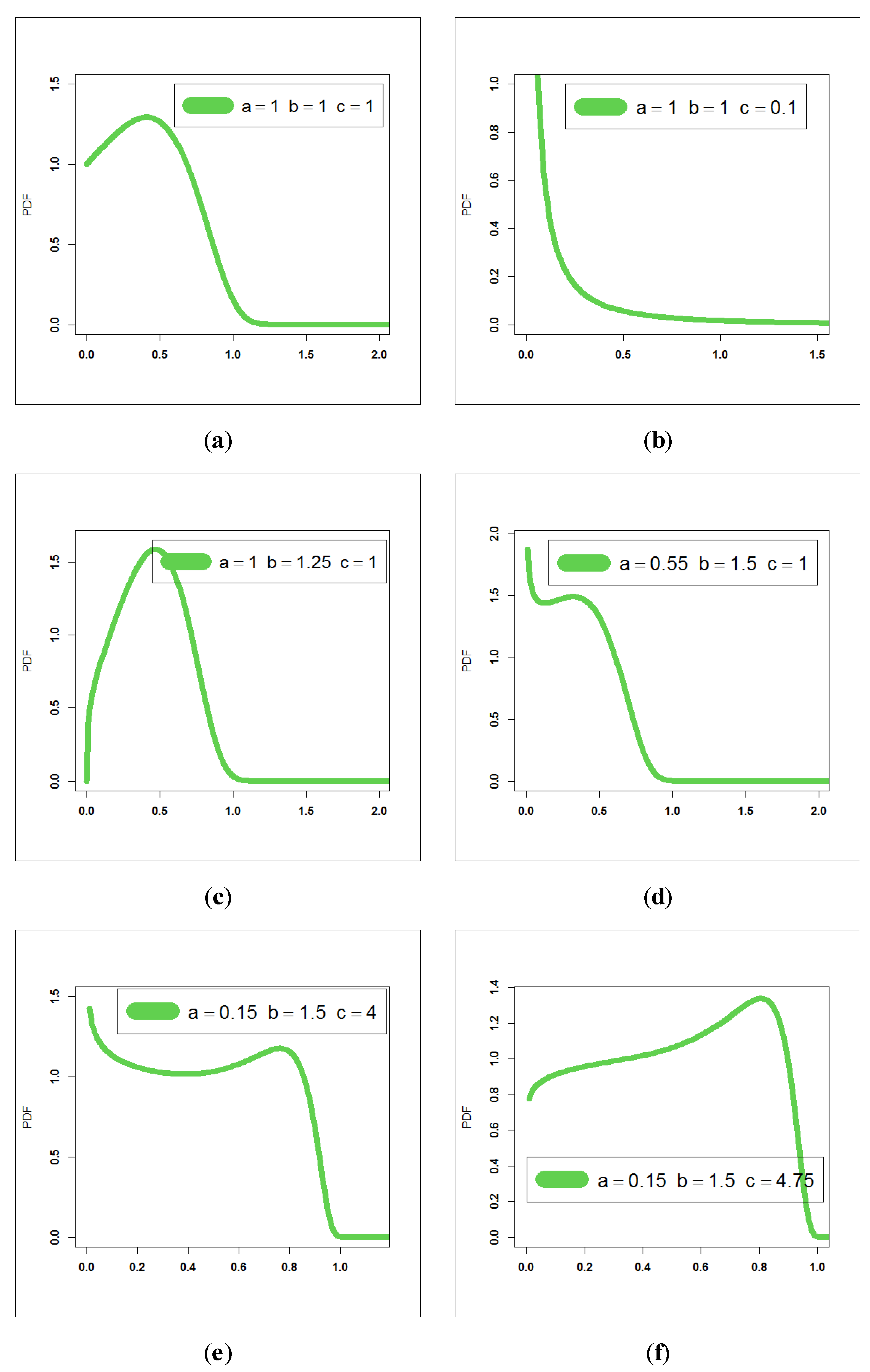
For exploring the flexibility of the new EWC PDF, we present Figure 1, which shows the wide flexibility of the new PDF of the EWC model.

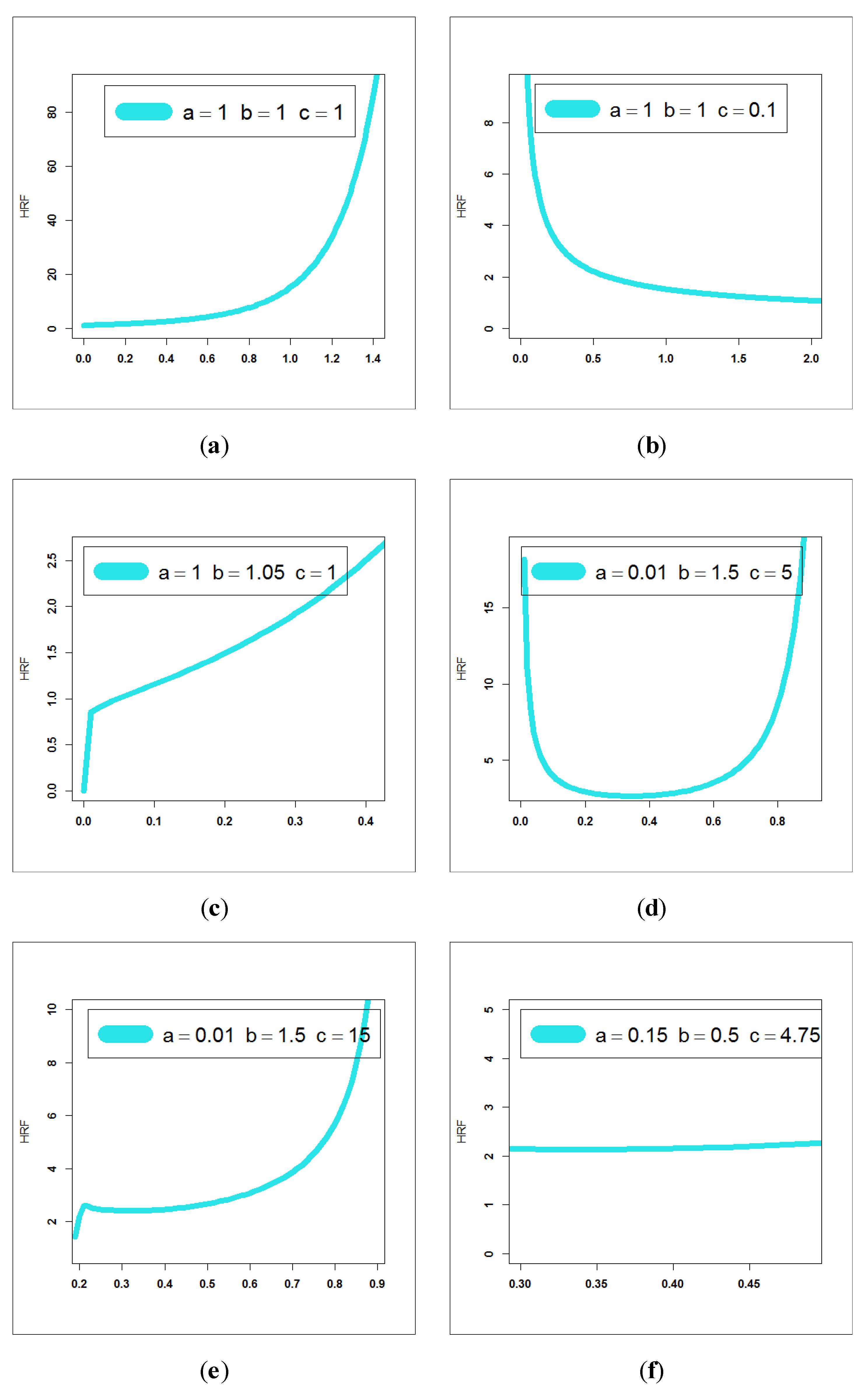
Based on Figure 1, we note that the new EWC PDF can be “symmetric”, “unimodal right skewed”, “unimodal left skewed”, “bimodal right skewed” and “bimodal left skewed” with different shapes. Analogously, Figure 2 is presented for exploring the flexibility of the HRF of the EWC model. Based on Figure 2, we note that the new EWC HRF can be “decreasing–constant–increasing (bathtub)”, “monotonically increasing”, “upside down constant–increasing”, “monotonically decreasing”, “upside down constant–increasing” and “upside down”.

We are motivated to define and study the EWC for the following reasons:

• The new PDF in (4) can be “unimodal right skewed with one peak”, “unimodal right skewed with no peak”, “unimodal left skewed”, “bimodal right skewed”, “symmetric” and “bimodal left skewed” with different shapes (see Figure 1).
• The HRF of the EWC model can be “decreasing–constant–increasing (bathtub)”, “monotonically increasing”, “upside down constant–increasing”, “monotonically decreasing”, “upside down constant–increasing” and “upside down” (see Figure 2).
• In reliability analysis, the EWC model may be chosen as the best probabilistic model, especially in modeling the right heavy tail bimodal asymmetric real data and left heavy tail bimodal asymmetric real data.

3. Linear Representation

In this section, we summarize and simplify the PDF and the CDF of the EWC model using some algebra such as the power series, the binomial expansion and generalized binomial expansion. Simplifying the PDF and the CDF of the EWC model helps us to derive many of its corresponding mathematical and statistical properties easily. Generally, our aim in this section is to re-express the PDF and the CDF of the EWC model in terms of the exponentiated base line model. After this, the mathematical and statistical properties of the EWC model can then be directedly derived from those corresponding mathematical and statistical properties of the exponentiated base line model.

If $\left|b_1\right|<1$ and $b_2>0$ is a real non-integer, the power series holds:

$${\left(1-b_1\right)}^{b_2-1} = \stackrel{+\infty }{\underset{b_3 = 0}{{{\displaystyle \sum }}^{ }}}\frac{{\left(-1\right)}^{b_3}\Gamma \left(b_2\right)}{i!\Gamma \left(b_2-b_3\right)}{b}_1^{b_3}.$$

(6)

Applying (6) to the last term in (4) gives

$$f_{\underset{\_}{V}}\left(x\right) = abc\frac{x^{c-1}\mathit{exp}\left(x^c\right){\overline{\sigma }}_c^{b-1}\left(x\right)}{{\sigma }_c^b\left(x\right)}\stackrel{+\infty }{\underset{i = 0}{{{\displaystyle \sum }}^{ }}}\frac{{\left(-1\right)}^i\Gamma \left(a\right)}{i!\Gamma \left(a-i\right)}\underset{A_{b,c}\left(x\right)}{\underbrace{\mathit{exp}\left[-\left(i+1\right){\left(\frac{\mathit{exp}\left\{\left[1-\mathit{exp}\left(x^c\right)\right]\right\}}{1-\mathit{exp}\left\{\left[1-\mathit{exp}\left(x^c\right)\right]\right\}}\right)}^b\right]}}.$$

(7)

Expanding the quantity $A_{b,c}\left(x\right)$, we can write

$$A_{b,c}\left(x\right) = \stackrel{+\infty }{\underset{\varsigma = 0}{{{\displaystyle \sum }}^{ }}}\frac{{\left(-1\right)}^{\varsigma }{\left(i+1\right)}^{\varsigma }}{\varsigma !}\frac{{\overline{\sigma }}_c^{\varsigma b}\left(x\right)}{{\sigma }_c^{\varsigma b}\left(x\right)}.$$

Inserting $A_{b,c}\left(x\right)$ in (7), then

$$f_{\underset{\_}{V}}\left(x\right) = abc{x}^{c-1}\mathit{exp}\left(x^c\right){\sigma }_c\left(x\right)\stackrel{+\infty }{\underset{i,\varsigma = 0}{{{\displaystyle \sum }}^{ }}}\frac{{\left(-1\right)}^{\varsigma +i}\Gamma \left(a\right){\left(i+1\right)}^{\varsigma }}{i!\varsigma !\Gamma \left(a-i\right)}\frac{{\overline{\sigma }}_c^{\left(\varsigma +1\right)b-1}\left(x\right)}{{\sigma }_c^{\left(\varsigma +1\right)b+1}\left(x\right)}.$$

(8)

Expanding ${\sigma }_c^{-\left[\left(\varsigma +1\right)b+1\right]}\left(x\right)$, we can write

$${\sigma }_c^{-\left[\left(\varsigma +1\right)b+1\right]}\left(x\right) = \stackrel{+\infty }{\underset{\zeta = 0}{{{\displaystyle \sum }}^{ }}}\frac{\Gamma \left(\left[\varsigma +1\right]b+\zeta +1\right)}{\zeta !\Gamma \left(\left[\varsigma +1\right]b+1\right)}{\overline{\sigma }}^{\zeta }\left(x\right).$$

(9)

Inserting (9) in (8), the EW-C density can then be expressed as

$$f_{\underset{\_}{V}}\left(x\right) = \stackrel{+\infty }{\underset{\varsigma ,\zeta = 0}{{{\displaystyle \sum }}^{ }}}{W}_{\varsigma ,\zeta } w_{\psi ,c}\left(x\right){|}_{\psi = \left(\varsigma +1\right)b+\zeta },$$

(10)

where

$$w_{\psi ,c}\left(x\right) = \psi h_c\left(x\right)H_c^{\psi -1}\left(x\right) = c{x}^{c-1}\mathit{exp}\left(x^c\right){\sigma }_c\left(x\right){\overline{\sigma }}_c^{\psi -1}\left(x\right)$$

is the exp-C pdf with power parameter $\psi$ and

$$W_{\varsigma ,\zeta } = \stackrel{+\infty }{\underset{i = 0}{{{\displaystyle \sum }}^{ }}}\frac{{\left(-1\right)}^{\varsigma +i}ab{\left(i+1\right)}^{\varsigma }\Gamma \left(a\right)\Gamma \left(\psi +1\right)}{\psi i!\varsigma !\zeta !\Gamma \left(a-i\right)\Gamma \left(\left[\varsigma +1\right]b+1\right)}.$$

In this regard, two theorems related to the Ex-C model are presented below:

Theorem 1.

Let $X$ be an RV with the Ex-C distribution with parameters $c$ and power parameter $\psi$. Then, using the transformation $t = {\left[G_c\left(x\right)\right]}^{\frac{1}{\psi }},$ the $sth$ ordinary moment of $X$ is given by

$${\mu }_{s,X}^{\prime } = E\left[X^s\right] = c{\displaystyle \sum }_{q_1,q_2 = 0}^{+\infty }{\psi }_{q_1}\left(\frac{s}{c}\right){\psi }_{q_2}\left(\frac{s}{c}+q_1\right)\frac{{\left(-1\right)}^{\frac{2s}{c}+q_1}}{\left[c\left(\psi +q_1+q_2\right)+s\right]},$$

where${\psi }_{q_1}\left(\frac{s}{c}\right)$is the coefficient of${\left[\mathit{log}\left(1-t\right)\right]}^{\frac{2s}{c}+q_1}$in the expansion of

$${\left\{{\displaystyle \sum }_{{\hslash }_1 = 1}^{+\infty }\frac{1}{{\hslash }_1}\left[\mathit{log}\left(1-t\right)\right]\right\}}^{\frac{s}{c}},$$

and${\psi }_{q_2}\left(\frac{s}{c}+q_1\right)$is the coefficient of$t^{q_1+q_2+\frac{s}{c}}$in the expansion of${\left({{\displaystyle \sum }}_{{\hslash }_2 = 1}^{+\infty }\frac{t^{{\hslash }_2}}{{\hslash }_2}\right)}^{\frac{s}{c}+q_1}$.

Theorem 2.

Let $X$ be an RV with the Ex-C distribution. Then, the $sth$ conditional moment can be derived as

$$E\left(X^s|X>x\right) = \psi c{\displaystyle \sum }_{q_1,q_2 = 0}^{+\infty }\frac{{\psi }_{q_1}\left(\frac{s}{c}\right){\psi }_{q_2}\left(\frac{s}{c}+q_1\right){\left(-1\right)}^{\frac{2s}{c}+q_1} {\sigma }_c\left(x\right)}{\left[c\left(\psi +q_1+q_2\right)+s\right]\left\{1-{\left[1-{\sigma }_c\left(x\right)\right]}^{\psi }\right\}}.$$

See [10] for more details.

4. Mathematical and Statistical Properties

4.1. Moments

Based on Theorem 1, the $s\mathrm{th}$ ordinary moment of the EWC model can then be expressed as

$${\mu }_{s,X}^{\prime } = E\left[X^s\right] = \psi c\stackrel{+\infty }{\underset{\varsigma ,\zeta ,q_1,q_2 = 0}{{{\displaystyle \sum }}^{ }{W}_{\varsigma ,\zeta }}}{\psi }_{q_1}\left(\frac{s}{c}\right){\psi }_{q_2}\left(\frac{s}{c}+q_1\right)\frac{{\left(-1\right)}^{\frac{2s}{c}+q_1}}{\left[c\left(\psi +q_1+q_2\right)+s\right]}.$$

(11)

4.2. The Conditional Moments

The conditional moments $E\left(X^s|X>x\right)$ can be expressed as

$$E\left(X^s|X>x\right) = \psi c\stackrel{+\infty }{\underset{\varsigma ,\zeta ,q_1,q_2 = 0}{{{\displaystyle \sum }}^{ }}}\frac{W_{\varsigma ,\zeta }{\psi }_{q_1}\left(\frac{s}{c}\right){\psi }_{q_2}\left(\frac{s}{c}+q_1\right){\left(-1\right)}^{\frac{2s}{c}+q_1}{\sigma }_c\left(x\right)}{\left[c\left(\psi +q_1+q_2\right)+s\right]\left\{1-{\left[1-{\sigma }_c\left(x\right)\right]}^{\psi }\right\}}.$$

(12)

In particular,

$$E\left(X|X>x\right) = \psi c\stackrel{+\infty }{\underset{\varsigma ,\zeta ,q_1,q_2 = 0}{{{\displaystyle \sum }}^{ }}}\frac{W_{\varsigma ,\zeta }{\psi }_{q_1}\left(\frac{1}{c}\right){\psi }_{q_2}\left(c+q_1\right){\left(-1\right)}^{\frac{2}{c}+q_1}{\sigma }_c\left(x\right)}{\left[c\left(\psi +q_1+q_2\right)+1\right]\left\{1-{\left[1-{\sigma }_c\left(x\right)\right]}^{\psi }\right\}},$$

and

$$E\left(X^2|X>x\right) = \psi c\stackrel{+\infty }{\underset{\varsigma ,\zeta ,q_1,q_2 = 0}{{{\displaystyle \sum }}^{ }}}\frac{W_{\varsigma ,\zeta }{\psi }_{q_1}\left(\frac{2}{c}\right){\psi }_{q_2}\left(\frac{2}{c}+q_1\right){\left(-1\right)}^{\frac{4}{c}+q_1}{\sigma }_c\left(x\right)}{\left[c\left(\psi +q_1+q_2\right)+2\right]\left\{1-{\left[1-{\sigma }_c\left(x\right)\right]}^{\psi }\right\}}.$$

4.3. Entropies

The Rényi entropy of the RV $X$ is defined by

$$I_{\delta }\left(X\right) = \frac{1}{\left(1-\delta \right)}\mathit{log}\left({{\displaystyle \int }}_{-\infty }^{+\infty }f{\left(x\right)}^{\delta }dx\right){|}_{\delta >0 \mathrm{and} \delta \ne 1}.$$

Using (4), we have

$$f_{\underset{\_}{V}}{\left(x\right)}^{\delta } = \stackrel{+\infty }{\underset{\varsigma ,\zeta = 0}{{{\displaystyle \sum }}^{ }}}{\tau }_{\varsigma ,\zeta }{x}^{c\delta -\delta }\mathit{exp}\left(\delta x^c\right)\mathit{exp}\left\{\delta \left[1-\mathit{exp}\left(x^c\right)\right]\right\}{\left\{1-\mathit{exp}\left[1-\mathit{exp}\left(x^c\right)\right]\right\}}^{b\varsigma +\zeta +\left(b-1\right)\delta },$$

where

$${\tau }_{\varsigma ,\zeta } = \stackrel{+\infty }{\underset{i = 0}{{{\displaystyle \sum }}^{ }}}\frac{{\left(-1\right)}^{i+\varsigma }{\left(cab\right)}^{\delta }{\left(\delta +i\right)}^{\varsigma }\Gamma \left(\left[a-1\right]\delta +1\right)\Gamma \left(b\varsigma +\left[b+1\right]\delta +\zeta \right)}{i!\varsigma !\zeta !\Gamma \left(b\varsigma +\left[b+1\right]\delta \right)\Gamma \left(\left[a-1\right]\delta -i+1\right)}.$$

Then,

$$I_{\delta }\left(X\right) = \frac{1}{\left(1-\delta \right)}\mathit{log}\left[\stackrel{+\infty }{\underset{\varsigma ,\zeta = 0}{{{\displaystyle \sum }}^{ }}}{\tau }_{\varsigma ,\zeta }{{\displaystyle \int }}_0^{+\infty }\left(\begin{array}{c}{x}^{c\delta -\delta }\mathit{exp}\left(\delta x^c\right)\mathit{exp}\left\{\delta \left[1-\mathit{exp}\left(x^c\right)\right]\right\}\\ \times {\left\{1-\mathit{exp}\left[1-\mathit{exp}\left(x^c\right)\right]\right\}}^{b\varsigma +\zeta +\left(b-1\right)\delta }\end{array}\right)dx\right].$$

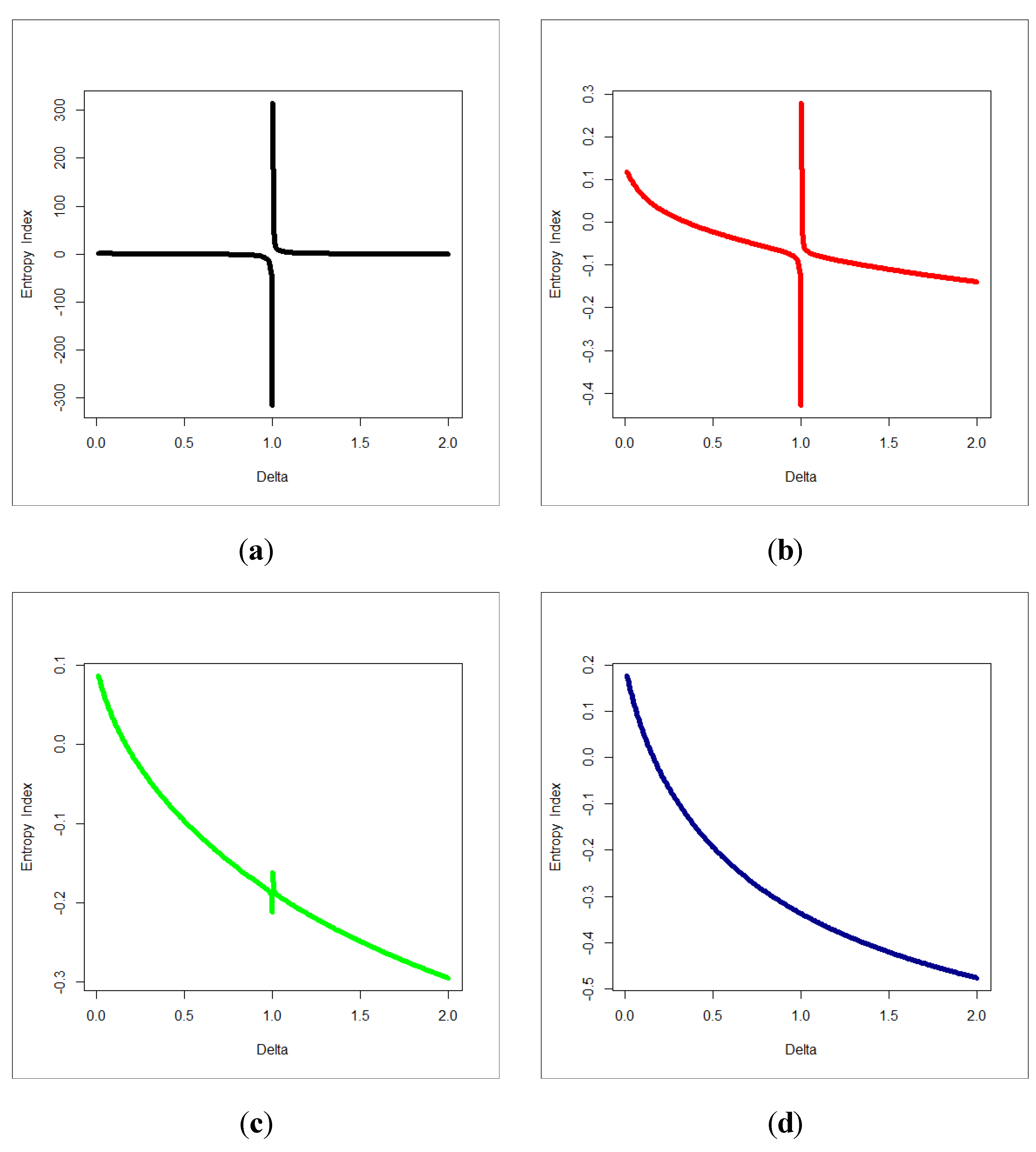
Figure 3 below gives the Rényi entropy index for the EWC model.

5. RIs

5.1. VaR Indicator

Exposure to risk certainly occurs for any insurance company. Hence, actuaries developed many risk indicators for evaluating exposure to risk numerically. Generally, the VaR is the amount of capital required to ensure, with a certain probability, that the company does not become insolvent technically. The degree of confidence chosen is arbitrary. Therefore, many VaR amount may be considered under several degrees of confidence. For the entire enterprise, it can be a high number such as $99.95\%$ or it can be $95\%$ for a single unit or risk class within the insurance company. These different percentages may reflect inter-risk type diversification or the inter-unit that exists. Let $X$ denote a loss RV (LRV). The VaR of $X$ (VaR$\epsilon$($X$)) at the $100\epsilon \%$ level, denoted as VaR$\epsilon \left(X\right)$ or $\pi \left(q\right)$, is the $100\epsilon$ quantile (or percentile) of the distribution of $X$. Then, for EWC distributions, we can simply write

$$\stackrel{\underset{}{}}{Pr}\left(X>\sqrt[c]{\mathit{log}\left[1-q\left(\epsilon ;a,b\right)\right]}\right) = \{\begin{array}{l}1\%{|}_{\epsilon = 99\%} \\ 5\%{|}_{\epsilon = 95\%} ,\\ ⋮ \end{array}$$

(13)

where $q\left(\epsilon ;a,b\right)=\mathit{log}\left(1-{\left\{1+\sqrt[b]{{\left[-\mathit{log}\left(1-\sqrt[a]{\epsilon }\right)\right]}^{-1}}\right\}}^{-1}\right)$. Based on (13), when $\epsilon = 99\%$ for a one-year time period, the interpretation is that there is only a very small chance ($1\%$) that the insurance company will be bankrupted by an adverse outcome over the next year. Then, the VaR$\epsilon \left(X\right)$ does not satisfy one of the four criteria for coherence.

5.2. TVaR Risk Indicator

Let $X$ denote an LRV. The TVaR$\epsilon \left(X\right)$ (TVaR$\epsilon$($X$)) at the $100\epsilon \%$ confidence level is the expected loss given that the loss exceeds $100\epsilon \%$ of the distribution of $X$. Then, the TVaR$\epsilon$($X$) can be expressed as

$$\epsilon \left(X\right) = E\left(X|X>\pi \left(\epsilon \right)\right) = \frac{1}{1-\epsilon }{{\displaystyle \int }}_{\pi \left(q\right)}^{+\infty }x{f}_{\underset{\_}{V}}\left(x\right)dx.$$

(14)

Then, depending on Theorem 2, we have

$$\epsilon \left(X\right) = \frac{\psi c}{1-\epsilon }\stackrel{+\infty }{\underset{\varsigma ,\zeta ,q_1,q_2 = 0}{{{\displaystyle \sum }}^{ }}}\frac{W_{\varsigma ,\zeta }{\psi }_{q_1}\left(\frac{1}{c}\right){\psi }_{q_2}\left(c+q_1\right){\left(-1\right)}^{\frac{2}{c}+q_1}{\sigma }_c\left(x\right)}{\left[c\left(\psi +q_1+q_2\right)+1\right]\left\{1-{\left[1-{\sigma }_c\left(x\right)\right]}^{\psi }\right\}},$$

(15)

where ${\psi }_{q_1}\left(\frac{1}{c}\right)$ is the coefficient of ${\left[\mathit{log}\left(1-t\right)\right]}^{\frac{2}{c}+q_1}$ in the expansion of ${\left\{{{\displaystyle \sum }}_{{\hslash }_1 = 1}^{+\infty }\frac{1}{{\hslash }_1}\left[\mathit{log}\left(1-t\right)\right]\right\}}^{\frac{1}{c}}$ and ${\psi }_{q_2}\left(\frac{1}{c}+q_1\right)$ is the coefficient of $t^{q_1+q_2+\frac{1}{c}}$ in the expansion of ${\left({{\displaystyle \sum }}_{{\hslash }_2 = 1}^{+\infty }\frac{t^{{\hslash }_2}}{{\hslash }_2}\right)}^{\frac{1}{c}+q_1}.$ Thus, TVaR $\epsilon \left(X\right)$ can be considered the average of all VaR values above the confidence level $q$. This means that TVaR $\epsilon \left(X\right)$ provides us more information about the tail of EWC distribution. Finally, TVaR can also be expressed as

$$e\left(\mathrm{VaR}\epsilon \left(X\right)\right) = \mathrm{TVaR}\epsilon \left(X\right)-\mathrm{VaR}\epsilon \left(X\right),$$

where $e\left(\mathrm{VaR}\epsilon \left(X\right)\right)$ is the mean excess loss function evaluated at the $100{\epsilon }^{th}$ quantile.

5.3. TV Risk Indicator

Let $X$ denote an LRV. The TV risk indicator (TV $\epsilon$ ($X$)) can be expressed as

$$\epsilon \left(X\right) = E\left(X^2|X>\pi \left(q\right)\right)-[\mathrm{TVaR}\epsilon \left(X\right){]}^2.$$

Then, depending on Theorem 2 and (15), we have

$$\epsilon \left(X\right) = \frac{\psi c}{1-\epsilon }\stackrel{+\infty }{\underset{\varsigma ,\zeta ,q_1,q_2 = 0}{{{\displaystyle \sum }}^{ }}}\frac{W_{\varsigma ,\zeta }{\psi }_{q_1}\left(\frac{2}{c}\right)w_{q_1,q_2}^2{\sigma }_c\left(x\right)}{w_{\left[2,\psi +q_1+q_2\right]}\left\{1-{\left[1-{\sigma }_c\left(x\right)\right]}^{\psi }\right\}}-{[\mathrm{TVaR}\epsilon \left(X\right)]}^2.$$

(16)

where $w_{q_1,q_2}^2 = {\psi }_{q_2}\left(\frac{2}{c}+q_1\right){\left(-1\right)}^{\frac{4}{c}+q_1}$, $w_{\psi +q_1+q_2}^2 = c\left(\psi +q_1+q_2\right)+2$ and TVaR$\epsilon \left(X\right)$ is given in (15).

5.4. TMV Risk Indicator

Let $X$ denote a loss of LRV. The TMV risk indicator (TMV$\epsilon$ ($X$)) can then be expressed as

$$\mathrm{TMV}\epsilon \left(X\right){|}_{0<\pi <1} = E\left(X^2|X>\pi \left(\epsilon \right)\right)-[\mathrm{TVaR}\epsilon \left(X\right){]}^2.$$

(17)

Then, for any LRV, TMV$\epsilon \left(X\right)>$ TV$\epsilon \left(X\right)$ and for $\pi = 1$ the TMV $\epsilon \left(X\right) =$ TVaR$\epsilon \left(X\right).$

6. Bimodal Asymmetric Data Applications

Let $x_1,x_2,\dots ,x_n$ be an observed random sample from the EW-C model with $\underset{\_}{V} = \left(a,b,c\right)$. The function of the log-likelihood according to the maximum likelihood estimation method can derived from

$${\ell }_{\underset{\_}{V}}\left(n\right) = \log \left\{{{\displaystyle \prod }}_{i = 1}^n\left[f_{\underset{\_}{V}}\left(x_i\right)\right]\right\}$$

The function of ${\ell }_{\underset{\_}{V}}\left(n\right)$ can be maximized directly using the “optim function” (using the R software) or sub-routine of MaxBFGS (using the program of Ox) or the MATH-CAD software or by solving the nonlinear equations of the likelihood derived from differentiating ${\ell }_{\underset{\_}{V}}\left(n\right)$. The score vector components $E_a = \frac{\partial }{\partial a}{\ell }_{\underset{\_}{V}}\left(n\right), E_b = \frac{\partial }{\partial b}{\ell }_{\underset{\_}{V}}\left(n\right)$ and $E_c = \frac{\partial }{\partial c}{\ell }_{\underset{\_}{V}}\left(n\right)$ can be easily derived from obtaining the nonlinear system $E_a = E_b = E_c = 0$ and then simultaneously solved to obtain the maximum likelihood estimates of $\underset{\_}{V}$. Using the “Newton–Raphson” algorithms, this system of equations can be solved numerically using iterative technique.

In this section, two real data sets are analyzed and considered under the maximum likelihood estimation (MLE) method for showing applicability of the EWC model. For comparing models, we consider the “$-\mathit{log}L$” Criteria, Akaike Information Criteria (AIC), the Consistent Information Criteria (CAIC), the Bayesian Information Criteria (BAIC), the Cramér–Von Mises (CvM) test and the Anderson–Darling (AD) test. Additionally, the Kolmogorov–Smirnov (K.S) test and its corresponding p-Value is also performed. The parameters of models have been estimated by the MLE method. The first data set (1.1, 1.4, 1.3, 1.7, 1.9, 1.8, 1.6, 2.2, 1.7, 2.7, 4.1, 1.8, 1.5, 1.2, 1.4, 3, 1.7, 2.3, 1.6, 2) is called the relief times of 20 patient data. The second data set (43.86, 44.97, 46.27, 51.29, 61.19, 61.20, 67.80, 69.00, 71.84, 77.31,85.39, 86.59, 86.66, 88.16, 96.03, 102.00, 108.29, 113.00, 115.14, 116.71, 126.86, 127.00, 127.14, 127.29, 128.00, 134.14, 136.14, 140.43, 146.43, 146.43,148.00, 148.43, 150.86, 151.29, 151.43, 156.14, 163.00, 186.43) is called the minimum flow. For more real data sets, see [11,12,13,14].

Table 1. Comparing models under the relief data set.

Model	BIC	AIC	AD	CVM	p-Value	K.S
EWC	40.62	37.63	0.241	0.042	0.952	0.116
GC	50.33	46.35	0.285	0.046	<0.01	0.992
BC	44.49	40.51	0.346	0.065	0.769	0.155
TC	56.62	53.63	1.575	0.274	0.243	0.233
KC	44.32	40.02	0.303	0.059	0.820	0.140
MOC	47.87	44.88	0.847	0.147	0.774	0.157
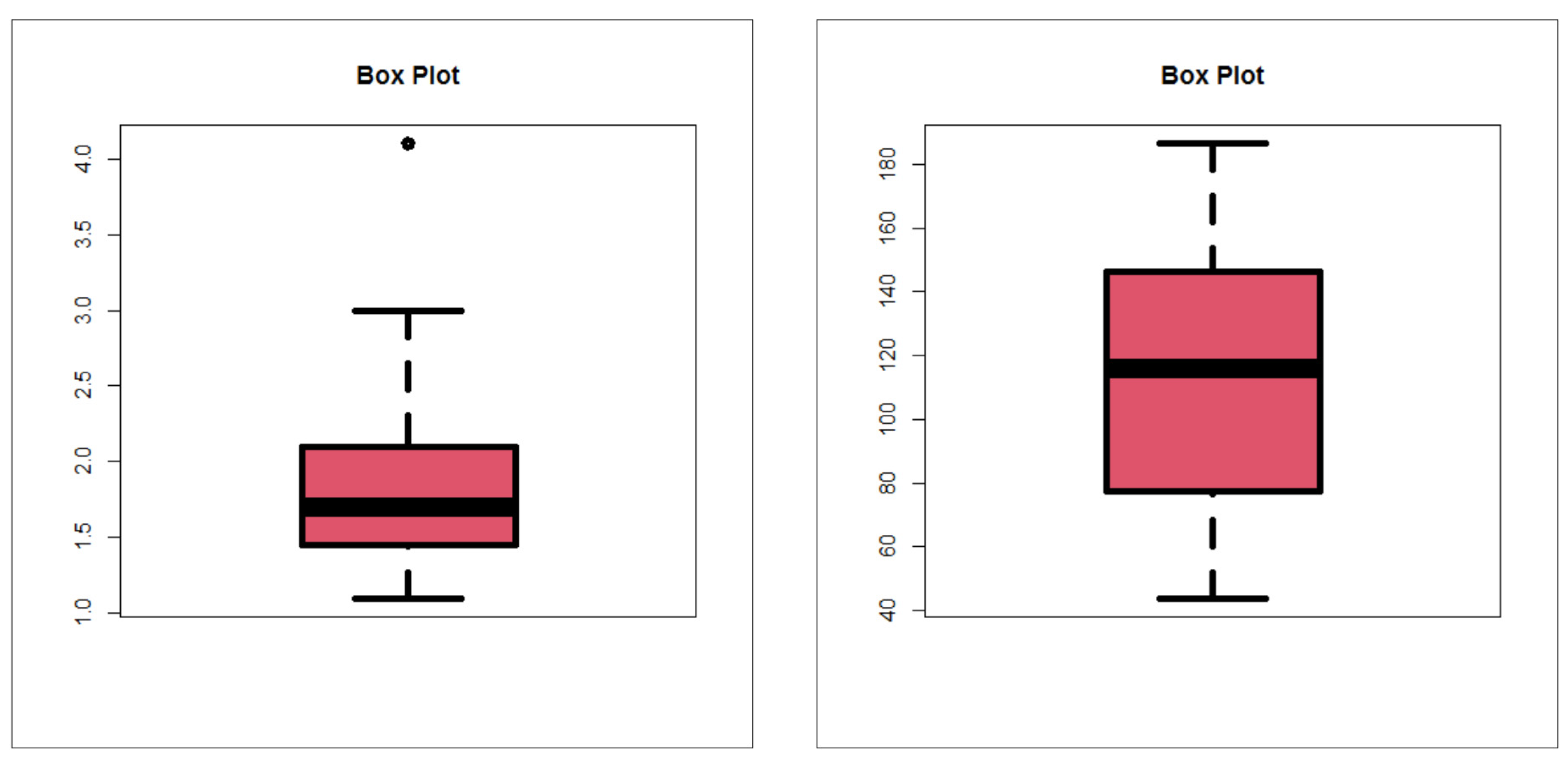
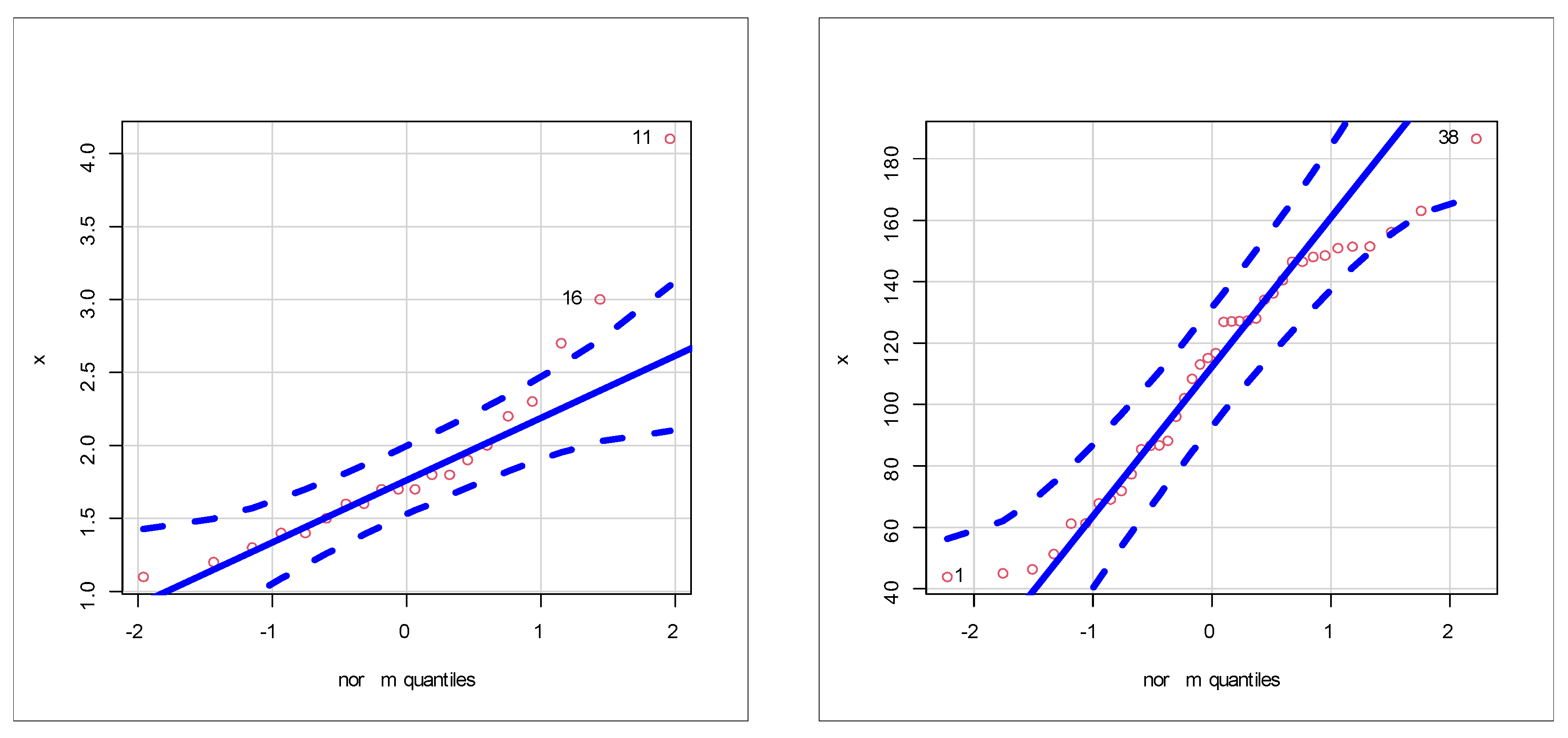
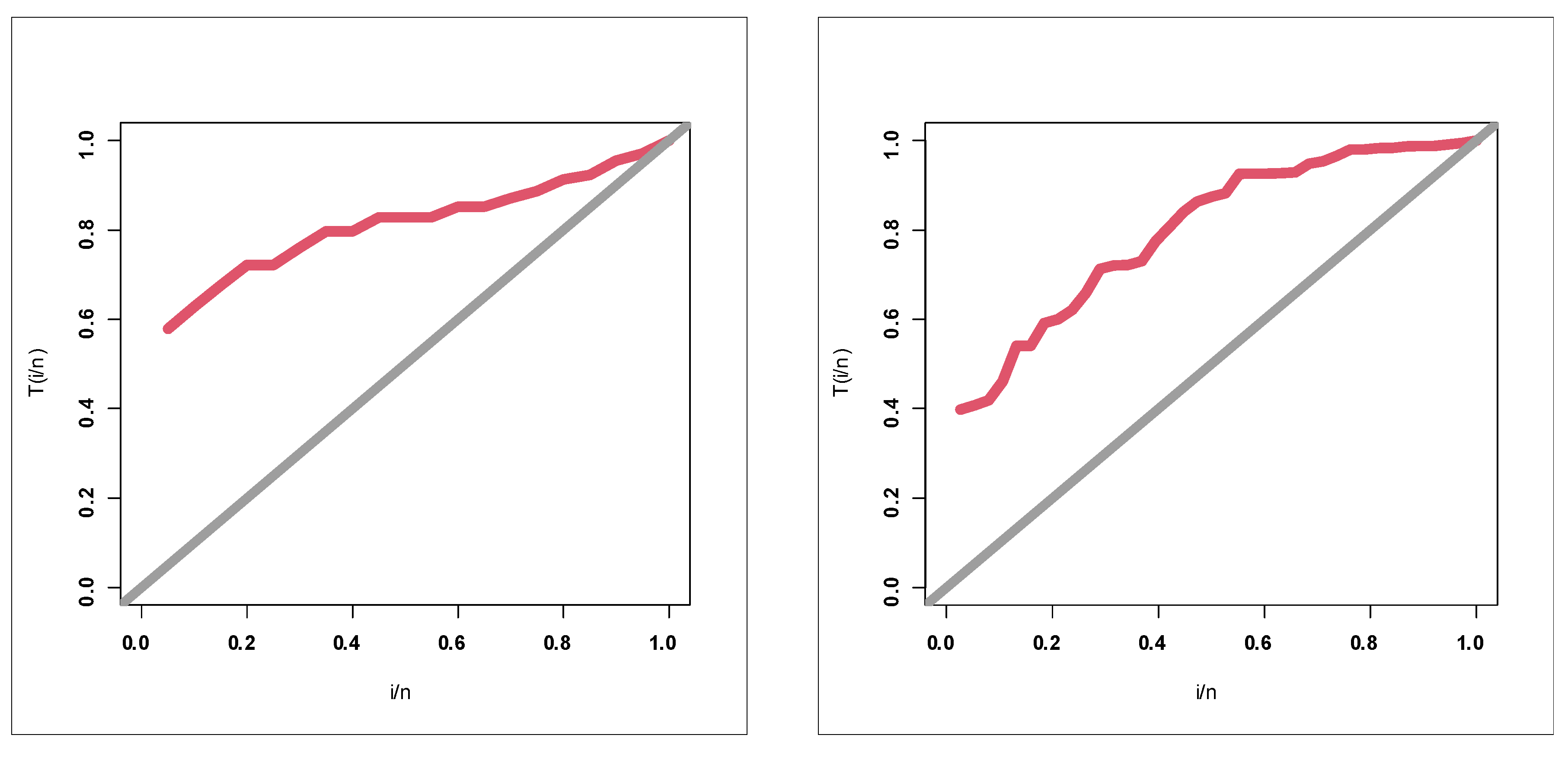
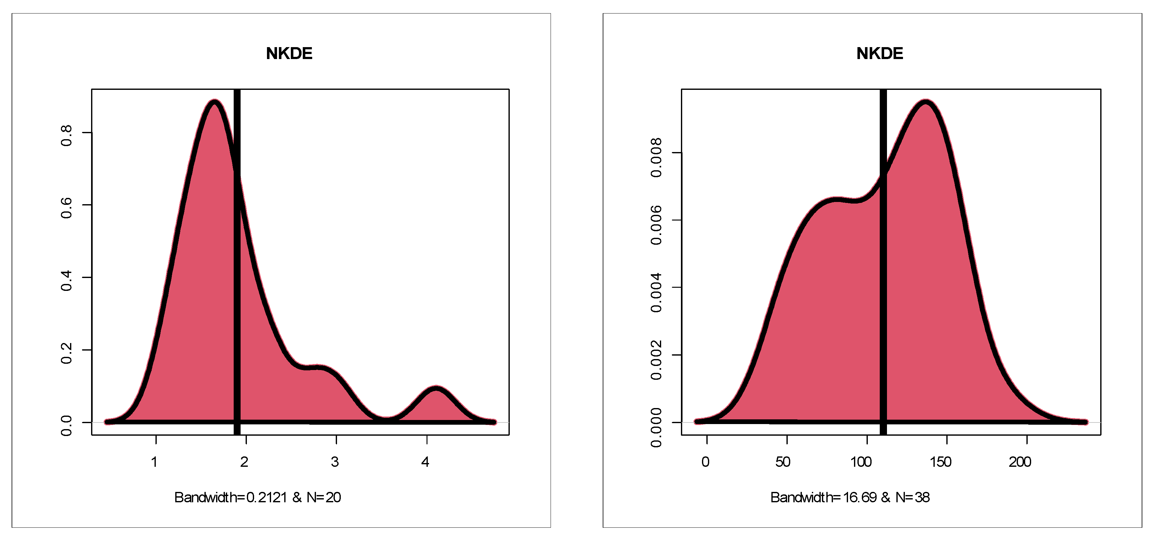
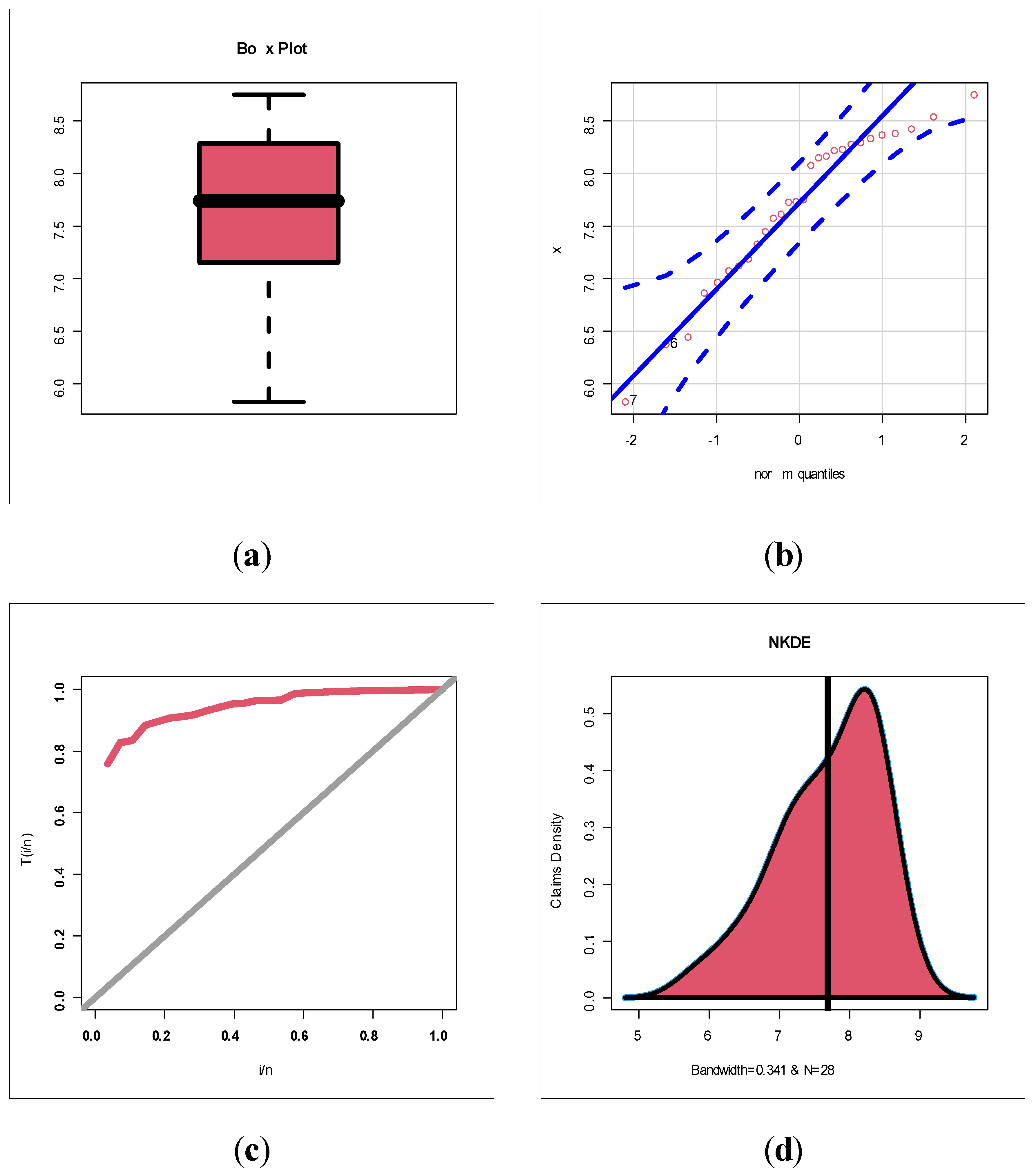
Chen	55.13	53.14	1.667	0.297	0.206	0.244

gives statistics tests for comparing the competing Chen extensions using the relief times real data set.

Table 2. The MLEs and SEs for the relief data set.

Model	MLE (SEs)
EWC(a,b,c)	1663.34, 1.167, 0.121
	(3.86), (2.487), (5.759)
GC(γ,a,b,c)	7.5914, 1.988, 5.0023, 0.534
	(2.09), (0.46), (1.07), (0.003)
MOC(a,b,c)	400.0123, 2.3243, 0.434
	(488.06), (0.64), (0.08)
KC(γ,a,b,c)	160.07, 0.491, 2.212, 0.5234
	(222.41), (0.51), (0.75), (0.21)
BC(γ,a,b,c)	85.873, 0.481, 2.013, 0.552
	(103.1), (0.512), (0.69), (0.20)
TC(a,b,c)	0.7455, 0.0714, 1.022
	(0.284), (0.034), 0.09)
Chen(b,c)	0.1388, 0.945
	(0.0511, 0.09)

lists the MLEs and their standard errors (SEs) for the relief times real data set. The competing Chen extensions listed in Table 1 and Table 2 are the EW-C (the proposed model), Gamma-Chen (GC), Kumaraswamy Chen (KC), Beta-Chen (BC), Marshall–Olkin Chen (MOC), Transmuted Chen (TC) and standard two-parameter Chen.

Table 3. Comparing models under the flow data set.

Model	BIC	AIC	AD	CVM	p-Value	K.S
EWC	394.37	389.36	0.60	0.11	0.705	0.11
MOC	395.47	390.56	0.61	0.09	0.689	0.12
GC	398.03	391.48	1.71	0.28	<0.01	0.57
Chen	401.90	398.62	0.64	0.10	0.262	0.16
BC	398.76	392.21	0.75	0.12	0.343	0.15
KC	397.79	391.24	0.66	0.11	0.409	0.14
TEC	398.29	391.74	0.70	0.11	0.377	0.15
TC	394.44	389.53	0.66	0.11	0.383	0.15
EC	394.82	389.91	0.72	0.13	0.348	0.15

gives statistics tests for comparing the competing models under the minimum flow data set.

Table 4. The MLEs and SEs for the minimum flow data.

Model	MLE (SEs)
EWC(a,b,c)	19.7987, 0.0537, 0.2449
	(4.66), (0.0049), (0.0036)
BC(γ,a,b,c)	3.014, 0.774, 0.014, 0.354
	(1.90), (1.24), (0.01), (0.05)
KC(γ,a,b,c)	4.514, 21.1104, 0.022, 0.273
	(2.02), (42.85), (0.02), (0.05)
GC(γ,a,b,c)	3.135, 4.364, 0.096, 0.345
	(1.143), (4.4), (0.02), (0.02)
MOC(a,b,c)	13.001, 0.0232, 0.3454
	(18.66), (0.02), (0.04)
EC(a,b,c)	2.859, 0.0144, 0.355
	(0.983), (0.004), (0.0234)
TEC(γ,a,b,c)	2.737, −0.248, 0.01, 0.348
	(1.213), (0.466), (0.01), (0.02)
TC(a,b,c)	−1.004, 0.0039, 0.368
	(0.70), (0.002), (0.01)
Chen(b,c)	0.0032, 0.365
	(0.001), (0.01)

lists the MLEs and SEs for the minimum flow data set. For describing the two real data sets, box plots, quantile–quantile (Q–Q) plots, total-time-in-test (TTT) plots and nonparametric-Kernel-density-estimation (NKDE) plots are presented. Figure 4 gives the box plots. Figure 5 gives the Q–Q plots. Figure 6 shows the TTT plots. Figure 7 gives the NKDE plots. The box plots show that the data for relief times have one extreme value (see Figure 5 left panel) and that the minimum flow data have one extreme value (see Figure 5 right panel). The Q–Q plots support the results obtained by the box plots. The dashed line in all of the Q–Q plots refers to the safe boundaries for the standard errors. The TTT plots show that the HRFs for the data on relief times are “monotonically increasing” (Figure 6 left panel) and that the HRFs for the data on relief times are “monotonically increasing” (see Figure 6 right panel). The NKDE plots show that the KDE is “asymmetric bimodal density” with a right tail (see Figure 7 left panel) and that the KDE of minimum flow data is “asymmetric bimodal density” (see Figure 7 right panel). The competing Chen extensions listed in Table 3 and Table 4 are the EW-C (the proposed model), Transmuted Exponentiated Chen (TEC), GC, KC, BC, MOC, TC and standard two-parameter Chen model.

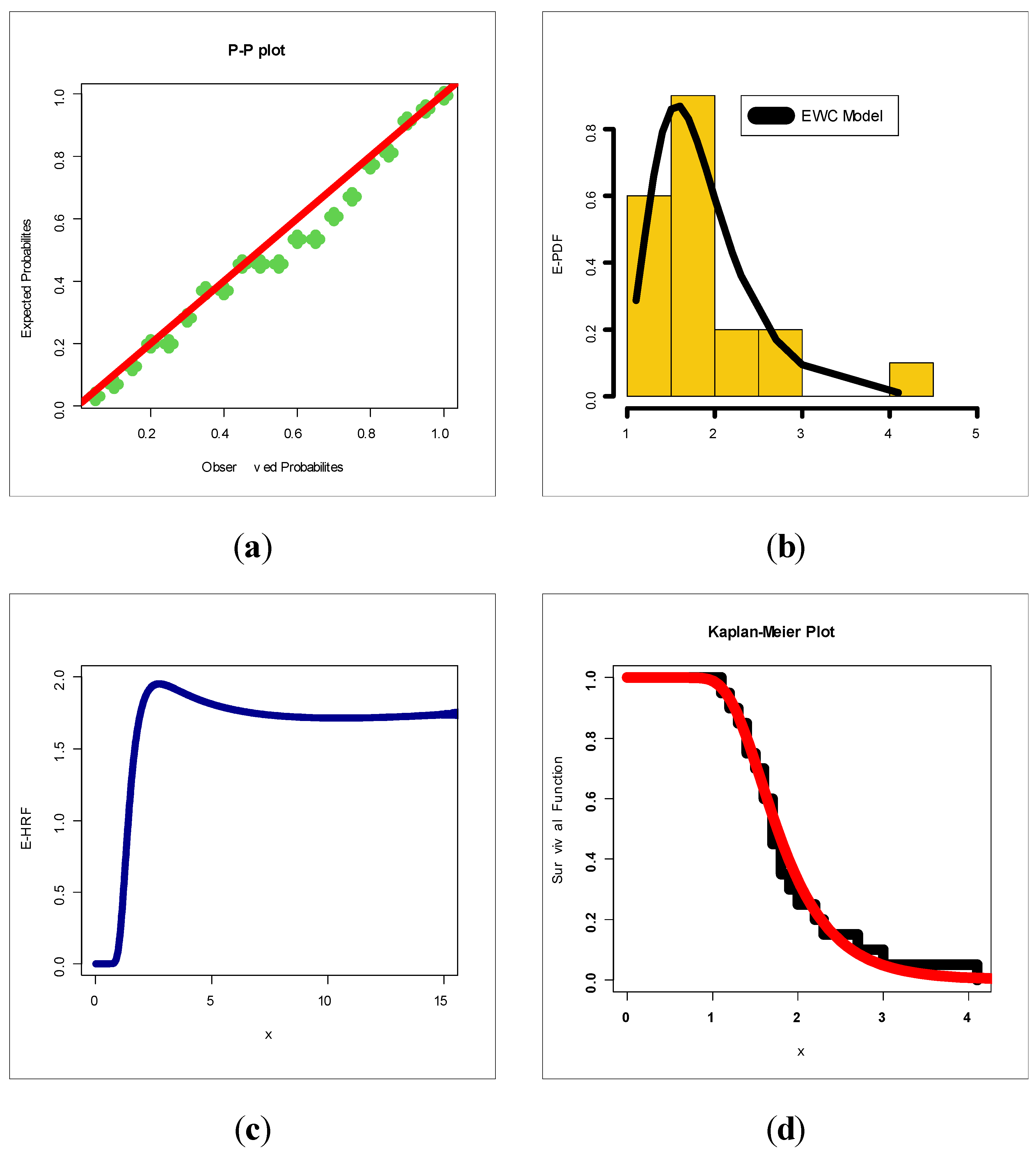
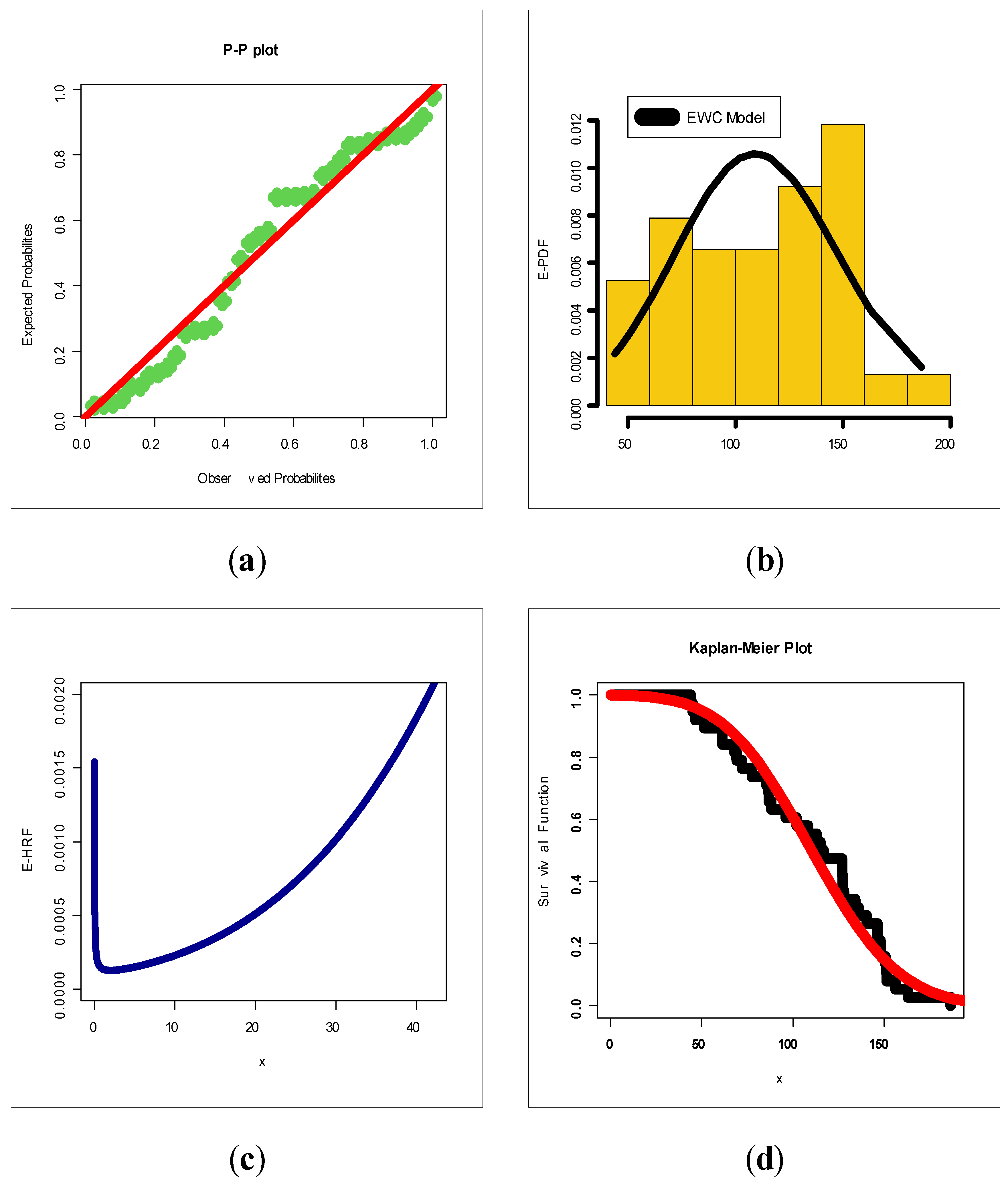
Based on Table 1, ${\mu }_{1,X}^{\prime }$ = 1.87197, variance = 0.3450812, skewness = 1.460947, kurtosis = 6.900911 and dispersion index = 0.1843413. Based on Table 1, ${\mu }_{1,X}^{\prime }$ = 0.008823, variance = 0.062213, skewness = 31.1491, kurtosis = 1024.202 and dispersion index = 7.050972. Based on Table 1, it is noted that the EWC model provides the best results: AIC = 37.63, BIC = 40.62, CVM = 0.042, AD = 0.241, K.S = 0.116 and p-value = 0.952. Table 3 gives the MLEs (SEs) for the data on relief times. Based on Table 3, it is noted that the EWC model provides the best results: AIC = 389.36, BIC = 394.37, CVM = 0.11, AD = 0.60, K.S = 0.11 and p-value = 0.705. Figure 7 and Figure 8 give the estimated-PDF (E-PDF), estimated-HRF (E-HRF), Probability–Probability (P–P) and the Kaplan–Meier survival plot for the relief times and the minimum flow data sets. According to Figure 8 and Figure 9, the new model showed a very close fit to the empirical functions in modeling the relief times and minimum flow data sets.

7. Risk and Time Series Analysis for Future Insurance-Claims Forecasting

Real data sets for insurance payments are usually positive and often has a right tail or a heavy right tail; it also can be unimodal (see [1,15,16,17] for more details). In this section, we analyze negatively skewed insurance-claims payment data for the first time under a new Chen extension. As illustrated in Section 2, the EWC density can be “symmetric”, “unimodal right skewed”, “unimodal and negatively skewed”, “bimodal and positively skewed” and “bimodal and negatively skewed” shapes. Since the insurance-claims data in the following subsection is a quarterly time series, we analyze the insurance-claims data using the AR(1) model. For exploring the autocorrelation between any two claims values, the autocorrelation function and the partial autocorrelation function plots are presented.

7.1. Insurance-Claims Application

In this section, we analyze the insurance-claims payment triangle from a U.K. motor non-comprehensive account; see [18]. We set the origin period as being from 2007 to 2013. The insurance-claims payment data frame presents the claims data in its typical form as it would be stored in a database. The first column presents the origin year from 2007 to 2013, the second column presents the development year and the third column has the incremental payments. It is worth mentioning that this insurance-claims data are first analyzed under a probability-based distribution. However, many other interesting insurance data can be analyzed using the new model; see, for example, [19] (for extreme value theory as a risk management tool with useful applications), [20] (for a review in skewed distributions in finance and actuarial science), [21] (for details about modeling claims data with composite Stoppa models), [22] (for more right censored medical and reliability data sets), [23] (for the jointly modeling area-level crash rates by severity with Bayesian multivariate random-parameters spatiotemporal Tobit regression), [24] (for the investigating the impacts of real-time weather conditions on freeway crash severity), [25] (for more copulas and a modified right censored test for validation) and [26] (for an alternative four-parameter exponentiated Weibull model with Copula, properties and real data modeling). For modeling the claims data, we first need to explore it. A real data set can be explored either numerically, graphically or both. In this section, we consider the numerical technique (see

Table 5. Statistical description for the insurance-claims data.

Statistic	Value
Mean	7.68589
Variance	0.54443
Skewness	−0.74828
Kurtosis	2.78846
Dis. Ix	0.07084
Median	7.74019
Length	28
Quantile (0.25%, 0.75%)	7.16935, 8.28125

) and many graphical techniques such as the Cullen–Frey plot for exploring initial fit to the theoretical common distributions such as uniform, normal, exponential, beta, lognormal, logistic and Weibull models. The bootstrapping method is also applied and plotted in the same plot. Note that the Cullen–Frey plot is used just to compare the models in the space of squared skewness and kurtosis. Many other graphical plots are used, such as the NKDE plot, the Q–Q plot, the TTT plot and the box plot. For exploring the autocorrelation between any two claims value, the autocorrelation function (ACF) plots are presented. The theoretical ACF and the partial ACF (Lag $= 1$) are also presented.

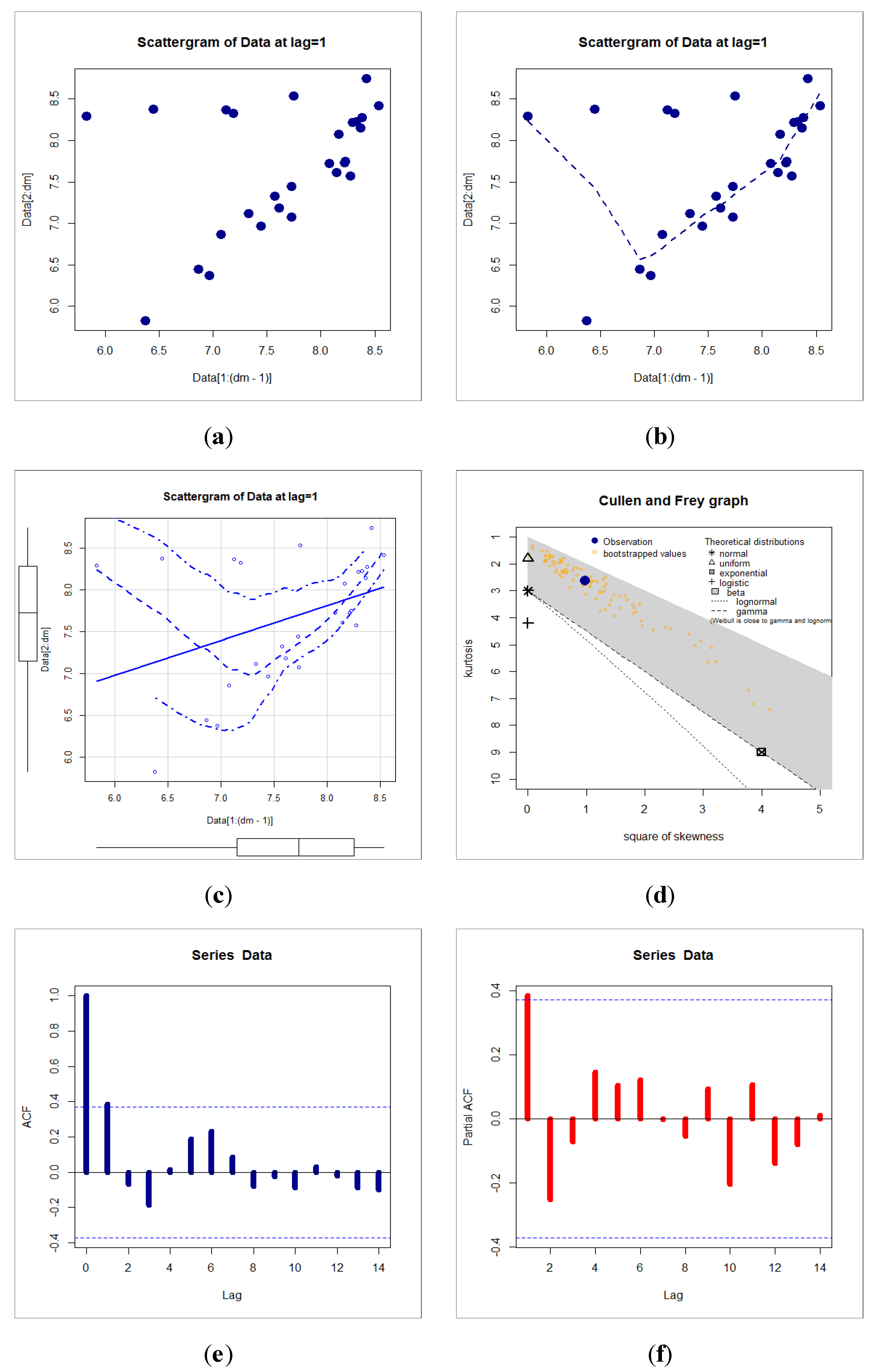
Figure 10 (top left) gives the box plot for the insurance claims. Figure 10 (top right) gives the Q–Q plot for the insurance claims. Figure 10 (bottom left) gives the TTT plot for the insurance claims. Figure 10 (bottom right) gives the NKDE plot for the insurance claims. Figure 11 (first, second and third plots) shows the scattergrams for insurance claims (Lag $= k = 1$). Figure 11 (fourth plot) gives the Cullen–Frey plot for the insurance claims. Based on Figure 11 (fourth plot), it is noted that we have left-skewed data and do not follow any of the above theoretical models. Figure 11 (fifth and sixth plots) gives the ACF (Lag $= k = 1$) and partial ACF (Lag $= k = 1$), respectively. Based on Figure 10 (top left and top right), we see that no extreme observations were spotted. Based on Figure 10 (bottom left), it is noted that the HRF of the claims is “monotonically increasing”. Figure 10 (bottom right) shows that the initial NKDE is an asymmetric function with a left tail. Based on Figure 11 (fifth and sixth plots), we note that that the first lag value (Lag $= k = 1$) is statistically significant, whereas the other partial autocorrelations for all other lags are not significant. Thus, the AR(1) model is suggested for the claims distribution. Table 5 below lists a statistical summary for the claims payment. Based on Table 5, it is noted that the Kurtosis of claims = 2.788464 $<$ 3, skewness of claims = $-$0.748278 (left-skewed claims data) and dispersion index of claims (Dis.Ix) = 0.0708352 (under dispersed claims data).

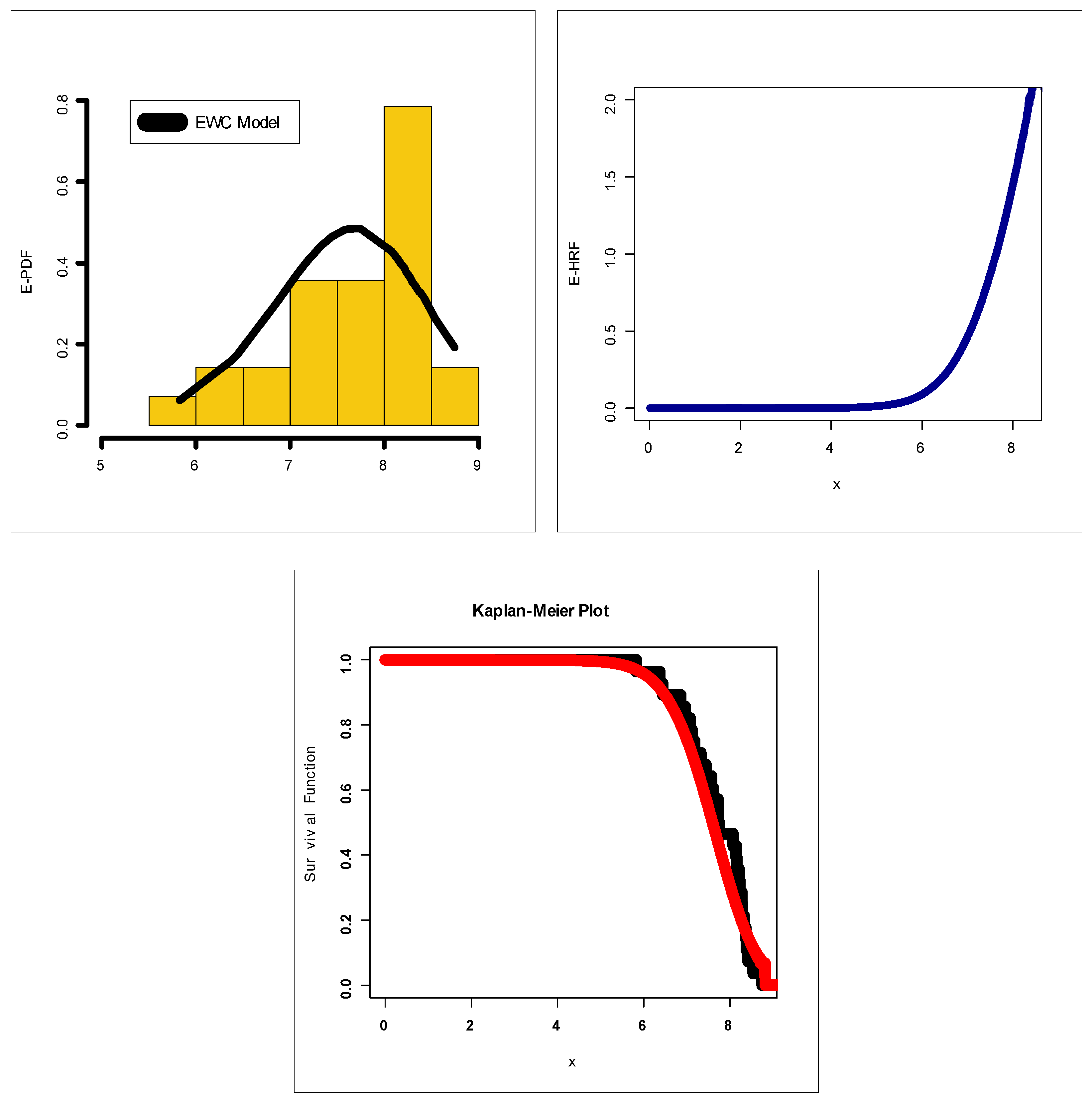
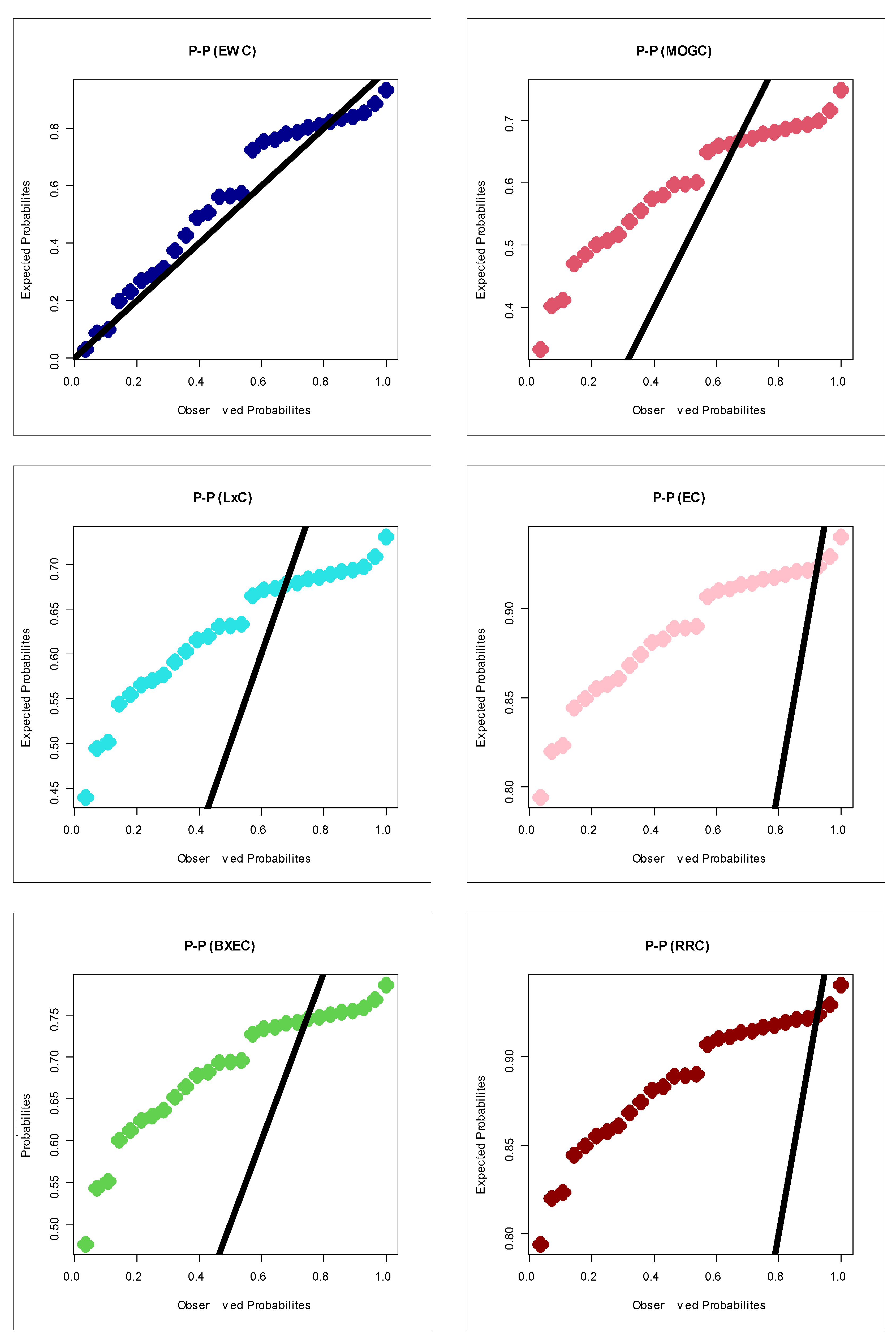
For modeling the insurance-claims data using a probability distribution, we consider some competitive potential probability distribution and hence compare those models with our new model under some goodness-of-fit test statistics. For this purpose, we consider some Chen extensions such as reduced Rayleigh Chen (RRC), the standard exponentiated distribution, the Burr X exponentiated Chen (BXEC) distribution, Burr XII Chen (BXIIC) distribution, Marshall–Olkin generalized Chen (MOGC) distribution, exponential Chen (EC), reduced Burr X Chen (RBXC), Weibull Chen (WC) and Lomax Chen (LxC) among others. The results of the statistical analysis for the insurance-claims data are presented in Table 2 and Table 3.

Table 6. Models, estimates and SEs for insurance-claims data.

Models	MLE (Standard Errors)
E(a)	0.130125
	(0.02459)
RRC(a)	0.0035352
	(0.000594)
EC(a)	0.0314453
	(0.005000)
RBXC(a,b)	1.11 × 103, 3.49 × 10−3
	(2.09 × 102), (5.85 × 10−4)
WC(a,b)	0.0280327, 0.593369
	(0.003384), (0.00187)
LxC(a,b)	0.0357072, 0.5933183
	(0.006761), (0.001931)
EWC(a,b,c)	30.859366, 0.0492140, 0.594392
	(8.163415), (0.002981), (0.00266)
BXIIC(a,b,c)	0.4928822, 0.0723965, 0.593369
	(1.817779), (0.267182), (0.00186)
BXEC(a,b,c,γ)	1.540293, 0.64830, 3.99381, 0.165361
	(0.34155), (0.186506), (0.88559), (0.0531)
MOGC(a,b,c,γ)	0.037152, 0.9789827, 0.316193, 0.7187880
	(0.01485), (0.48380), (0.0024), (0.00190)

gives the competitive models, estimates and standard error (SEs) for insurance-claims data.

Table 7. Comparing models under the insurance data set.

Models	BIC	AIC	AD	CvM	K.S (p-Value)
EWC	71.51872	67.52211	0.6173	0.1008	0.18832 (0.2416)
BXEC	142.6455	137.3167	0.7658	0.12082	0.5073 (3 × 10−7)
BXIIC	139.7025	135.7059	0.6819	0.1092	0.45878 (7 × 10−6)
MOGC	121.0229	115.6941	0.6353	0.1028	0.36671 (6 × 10−7)
E	173.538	172.2056	0.8219	0.12899	0.5316 (6.5 × 10−8)
WC	173.9965	171.3321	0.5077	0.0865	0.7932 (7.8 × 10−16)
EC	461.0206	459.6884	0.8588	0.1345	0.9961 (8 × 10−16)
RRC	1383.541	1382.209	0.8721	0.1365	1 (8 × 10−16)
RBXC	994.1684	991.504	0.8732	0.1366	1 (8 × 10−16)

lists the test statistics for insurance-claims data. Figure 7 presents estimated PDF (E-PDF), estimated HRF (E-HRF) and Kaplan–Meier survival plots for insurance-claims data. Figure 7 gives the probability–probability (P–P) plots for all of the competitive models. Based on Figure 12 (left panel), it is seen that the E-PDF of the EWC fits the histogram of the insurance-claims payments and that the two shapes are negative skewed. Based on Figure 12 (middle panel), it is seen that the E-HRF is increasing. Based on Figure 12 (right panel), it is seen that the estimated survival function of the EWC fits the Kaplan–Meier survival plot of the insurance-claims data. Based on Figure 12 (the E-PDF, E-HRF and the Kaplan–Meier survival plots), it is seen that the EWC model provided an adequate fit to the negative skewed claims payments. According to the P–P plots (see Figure 13), one can clearly note that the EWC model is the most reasonable probability model out of all other competitive Chen models. Based on Table 6 under the AIC, BIC, CvM, AD, the Kolmogorov–Smirnov test and its corresponding p-value (under the chi-square goodness-of-fit test), the EWC model is the best among all competitive Chen models.

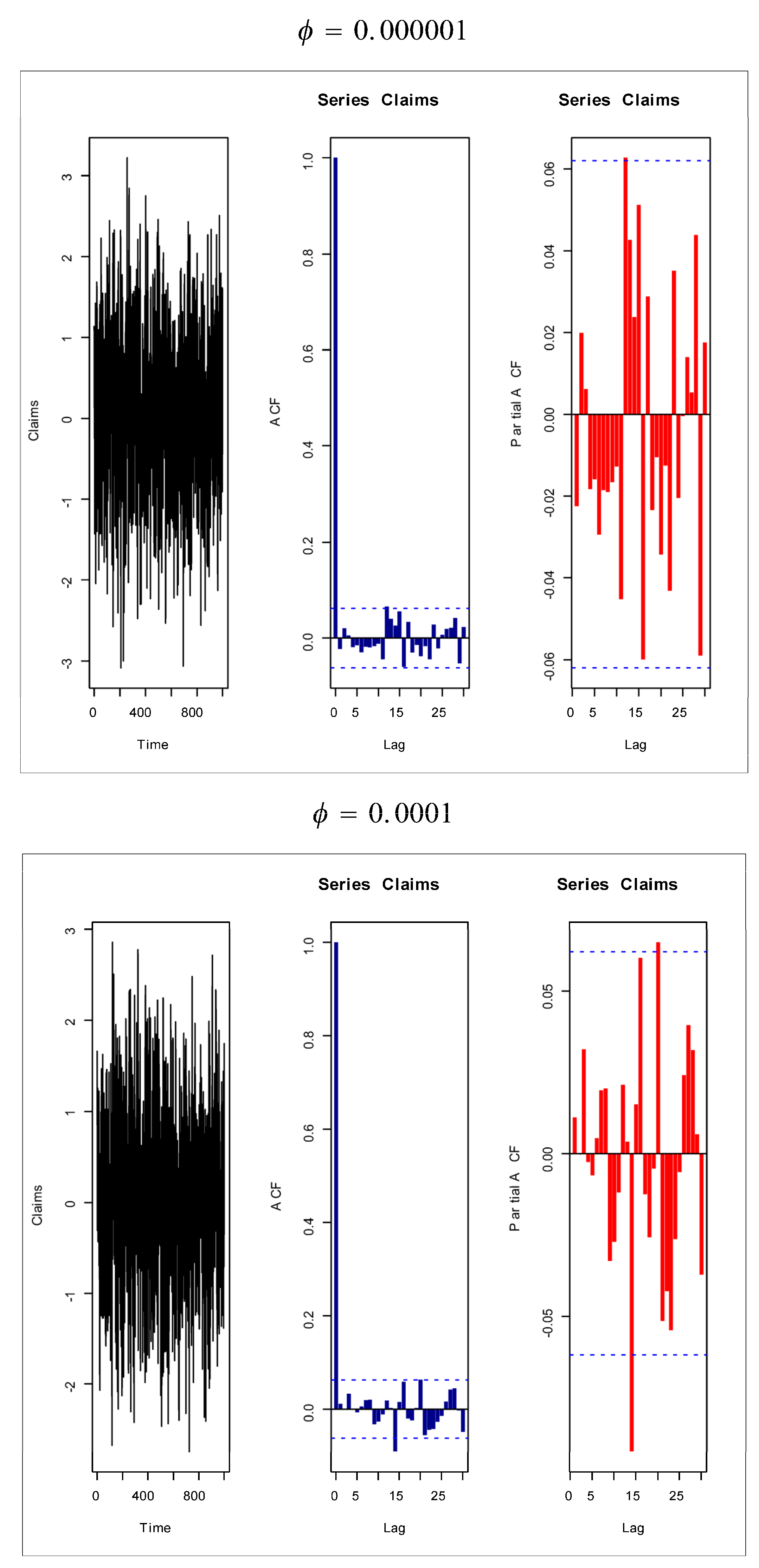
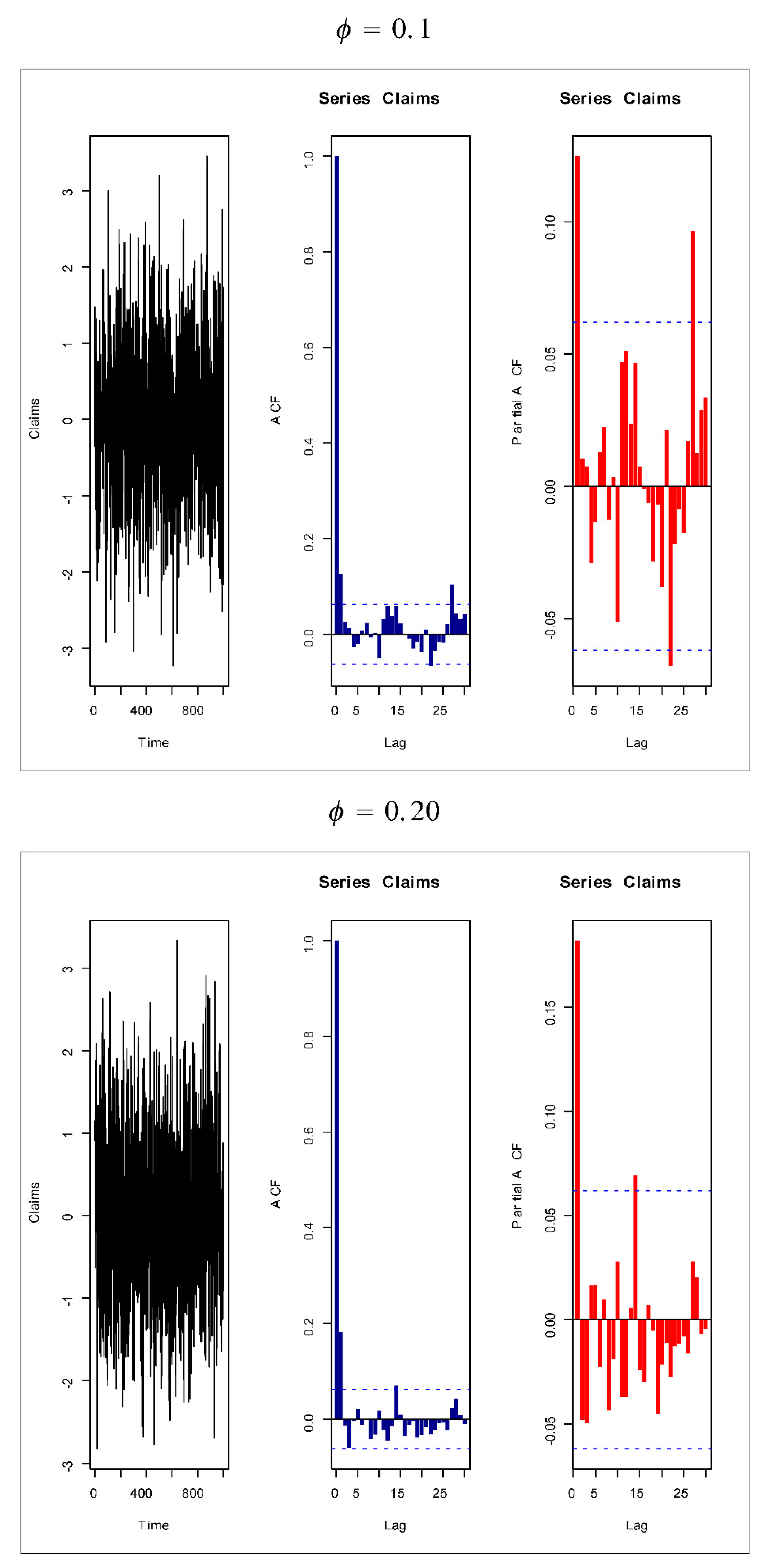
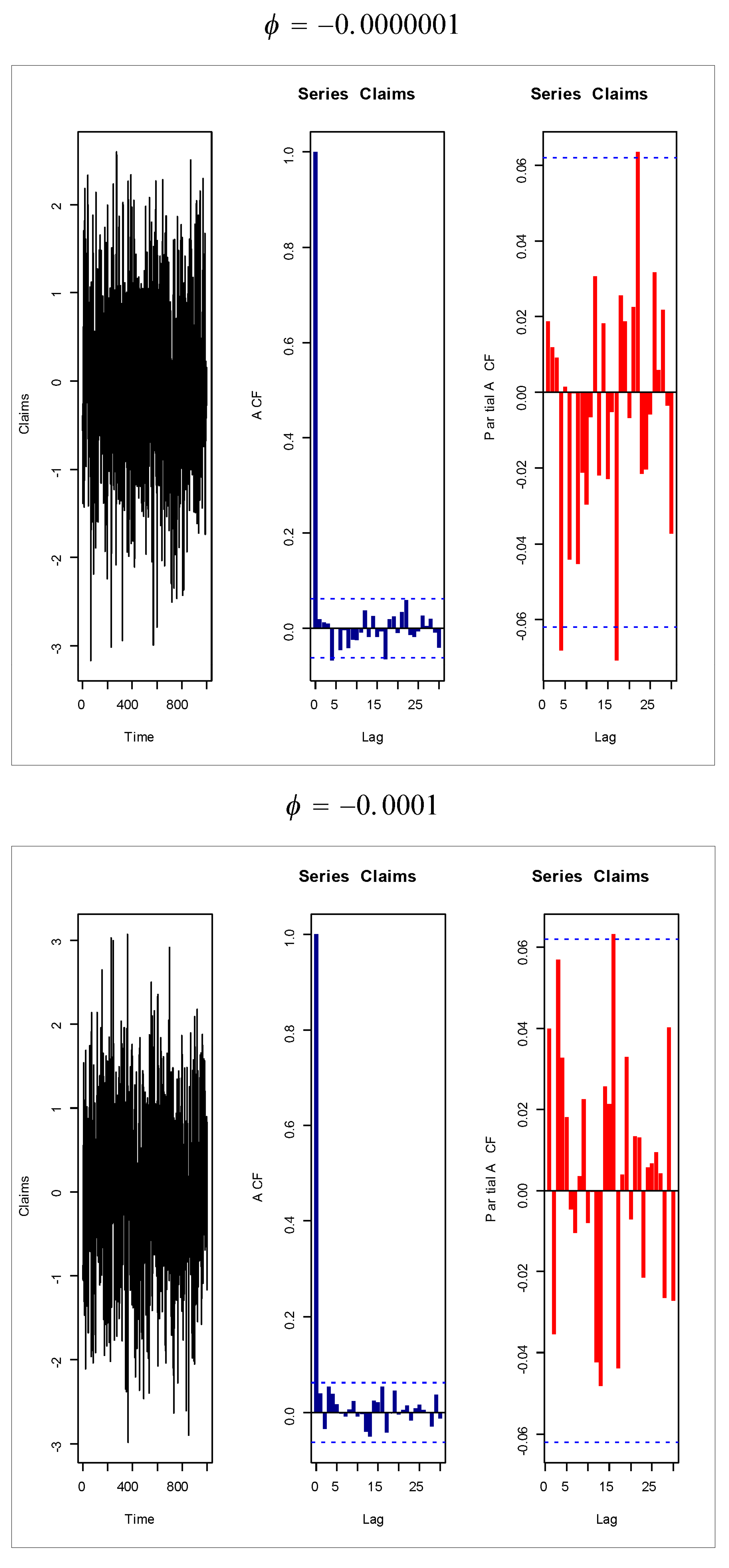
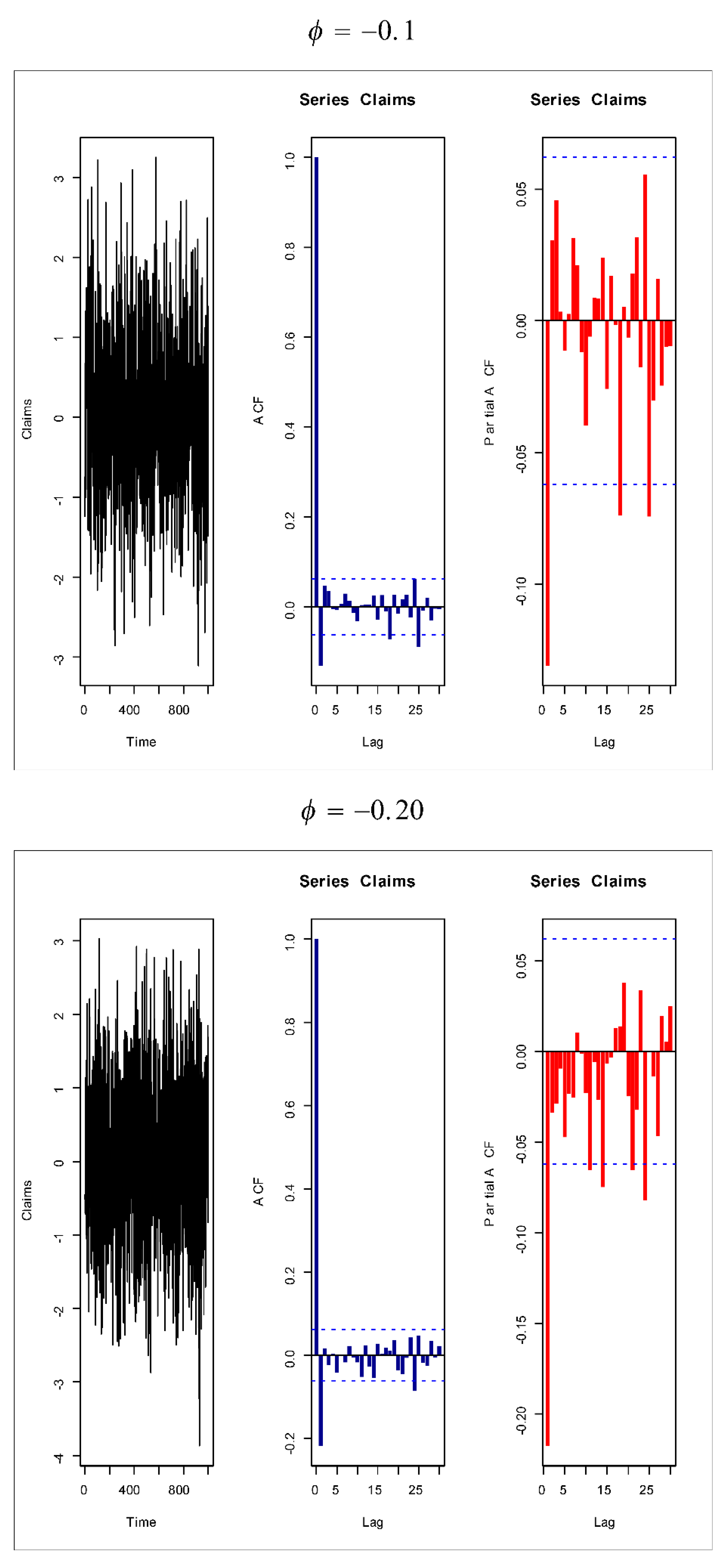
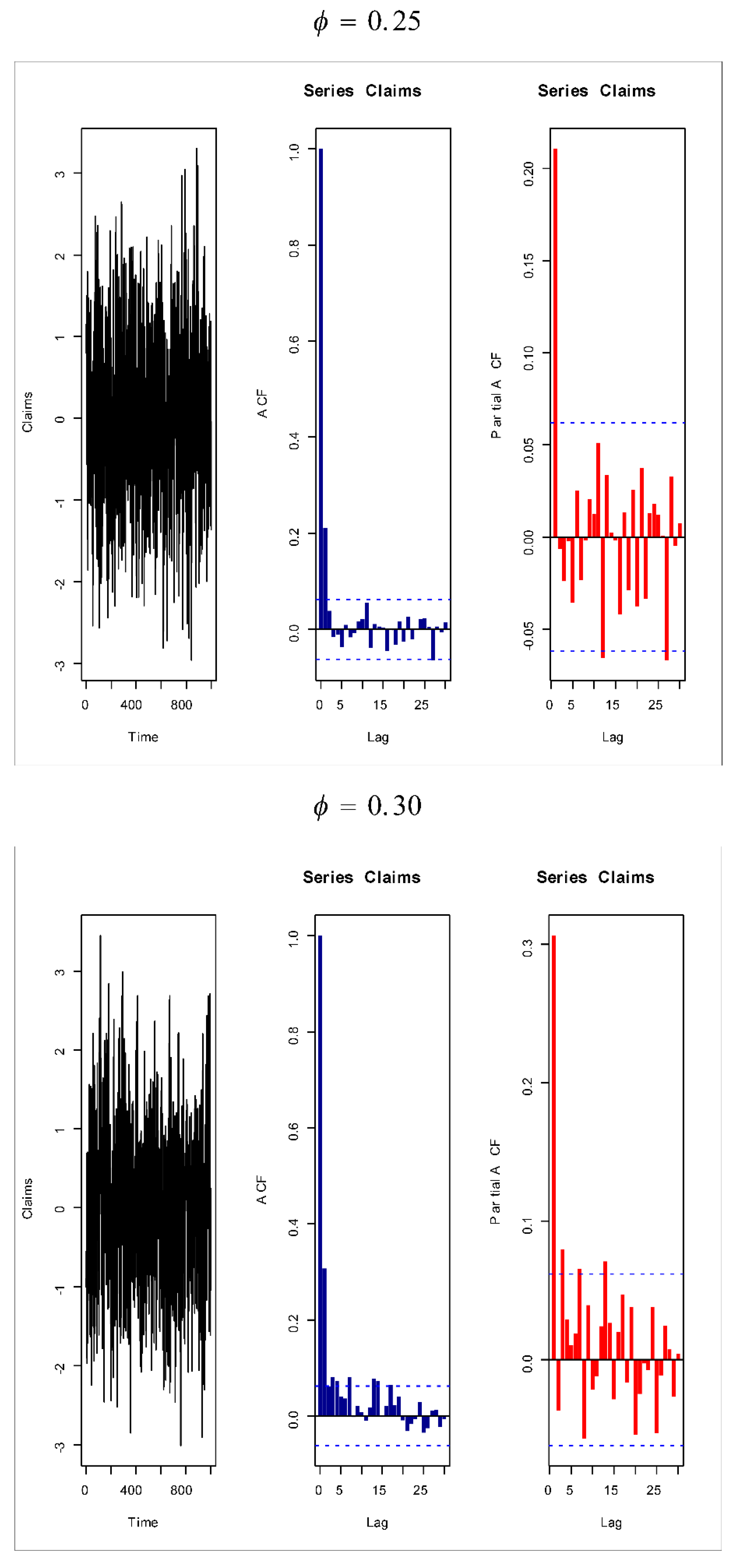
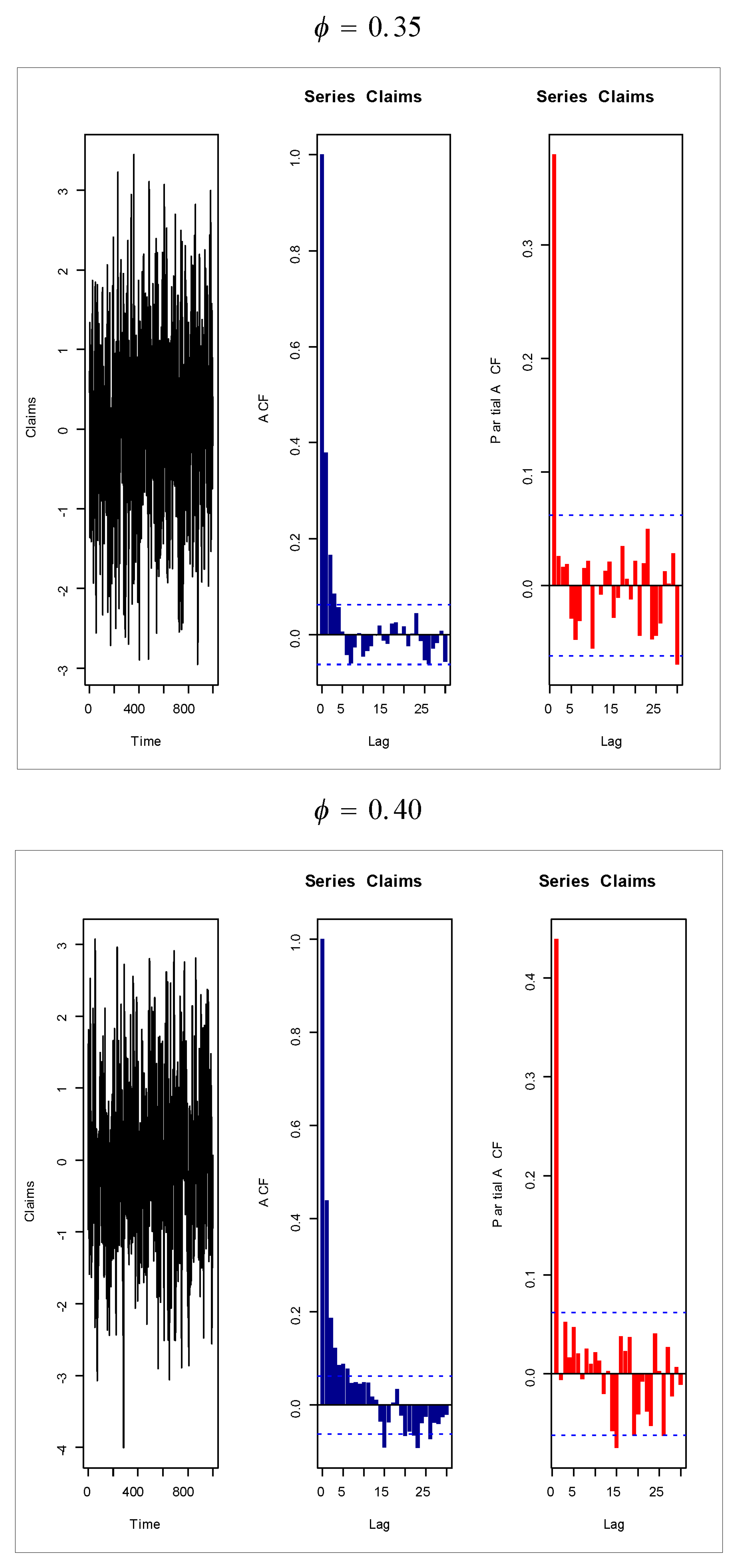
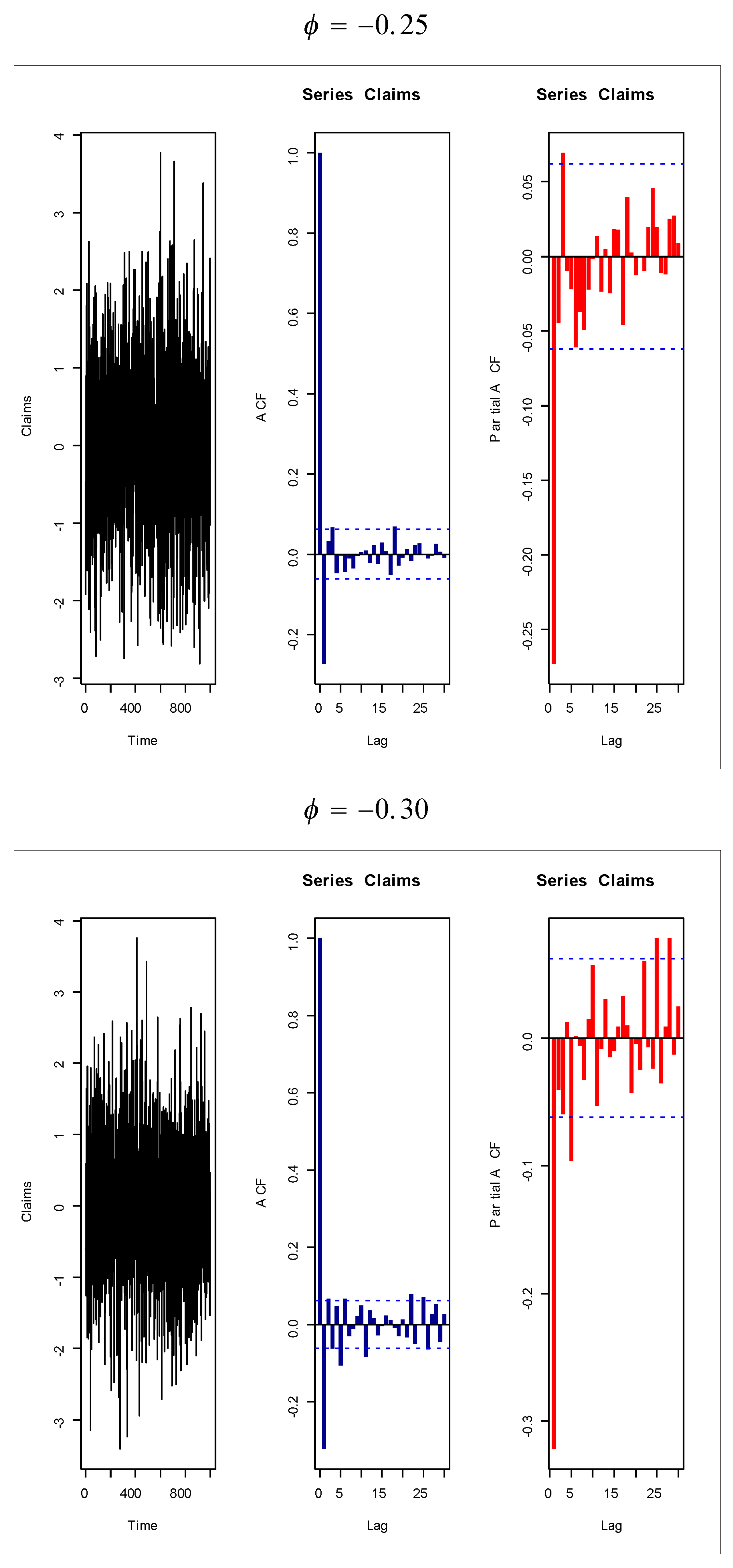
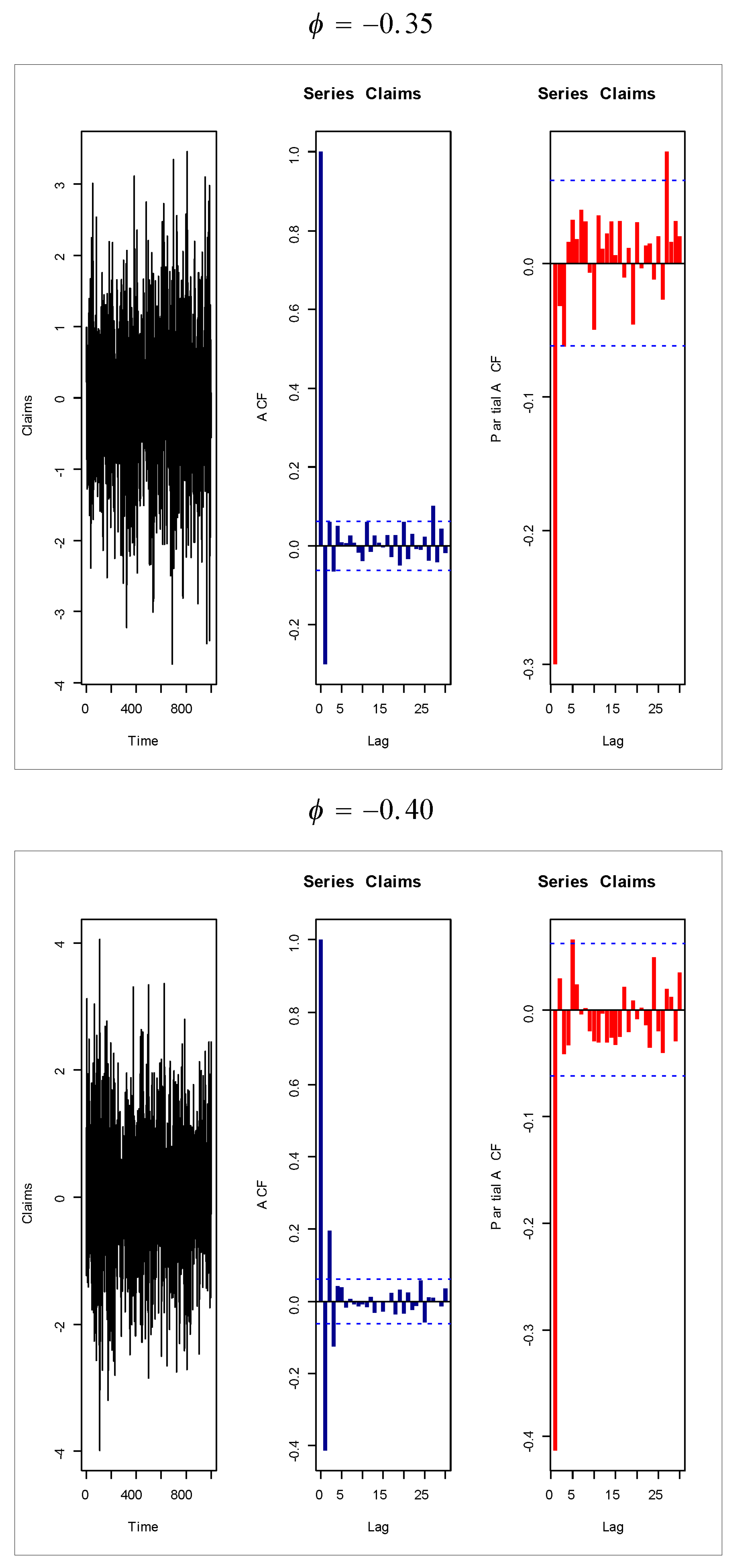
Based on Figure 1 (fifth and sixth plots), the AR(1) model is suggested to present the insurance-claims payments. Figure 14, Figure 15, Figure 16 and Figure 17 give some artificial claims payments with ACF (${\rho }_{\left[k\right]}$) and partial ACF (${\Phi }_{\left[kk\right]}$) generated based on some positive and negative values of the parameter $\phi$ = $\left(\pm {10}^{-7},\pm {10}^{-4},\pm 0.10,\pm 0.20\right)$. Figure 18, Figure 19, Figure 20 and Figure 21 give some artificial claims payments with ACF (${\rho }_{\left[k\right]}$) and partial ACF (${\Phi }_{\left[kk\right]}$) generated based on some positive and negative values of the parameter $\phi$ = $\left(\pm 0.25,\pm 0.30,\pm 0.35,\pm 0.40\right)$. For a positive value of the parameter $\phi$ (${\phi }^{+}$) the ACF $\to 0$ exponentially as lag $\to$+$\infty$. For negative values of the parameter $\phi$ (${\phi }^{-}$), the ACF $\to 0$ exponentially as lag $\to$+$\infty$. For a positive value of the parameter $\phi$, the partial ACF shuts off after the first lag since $\phi <1$. For negative values of the parameter $\phi$, the partial ACF shuts off after the first lag since $\phi <1$.

Table 8. Point prediction for the claims payments in millions.

Forecasting→	${\mathit{\rho }}_{\mathbf{\left[}\mathit{k}\mathbf{\right]}}{\mathbf{|}}_{\mathit{k}\mathbf{\ge }\mathbf{1}}$				${\mathit{\Phi }}_{\mathbf{\left[}\mathbf{11}\mathbf{\right]}}$	Point Forecasting
φ↓	1	2	3	4		y29	y30	y31
10−7	10−7	10−14	10−21	10−28	10−7	7.685890	7.68589	7.68589
−10−7	−10−7	10−14	−10−21	10−28	−10−7	7.685890	7.68589	7.68589
+10−4	10−4	10−8	10−12	10−16	10−4	7.685996	7.68589	7.68589
−0.10−4	−10−4	10−8	−10−12	10−16	−10−4	7.685784	7.68589	7.68589
+0.10	+0.1	10−2	+10−3	10−4	0.10	7.791861	7.696487	7.68695
−0.10	−0.1	10−2	−10−3	10−4	−0.10	7.579919	7.696487	7.68483
+0.20	0.20	0.04	0.008	0.0016	0.20	7.897833	7.728279	7.694368
−0.20	−0.20	0.04	−0.008	0.0016	−0.20	7.473947	7.728279	7.677412
+0.25	0.25	0.0625	0.0156	0.00391	0.25	7.950818	7.752122	7.702448
−0.25	−0.25	0.0625	−0.0156	0.00391	−0.25	7.420962	7.752122	7.669332
+0.30	0.3	0.09	0.027	0.0081	0.3	8.003804	7.781264	7.714502
−0.30	−0.3	0.09	−0.027	0.0081	−0.3	7.367976	7.781264	7.657278
+0.35	0.35	0.1225	0.04288	0.0150	0.35	8.05679	7.815705	7.731325
−0.35	−0.35	0.1225	−0.04288	0.0150	−0.35	7.31499	7.815705	7.640455
+0.40	0.40	0.16	+0.64	0.0256	0.40	8.109775	7.855444	7.753712
−0.40	−0.40	0.16	−0.64	0.0256	−0.40	7.262005	7.855444	7.618068

provides the point prediction (the future values $y_{29},$ $y_{30}$ and $y_{31}$) for the claims payments in millions. In Table 8, ${\rho }_{\left[k\right]}{|}_{k\ge 1}$ and ${\Phi }_{\left[11\right]}$ are also calculated for each value of $\phi$.

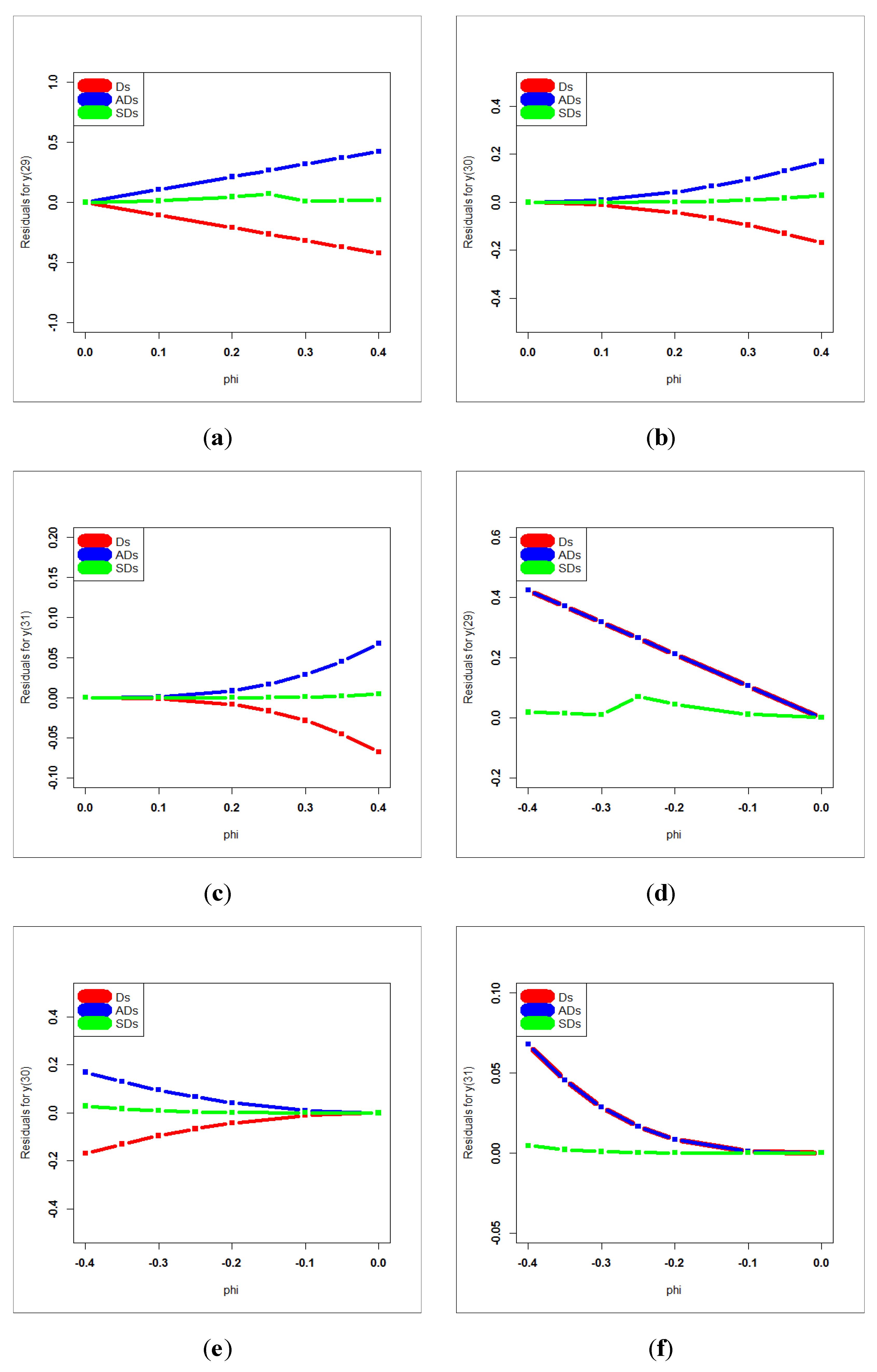
The future values $y_{29},$ $y_{30}$ and $y_{31}$ are very important for the insurance companies for avoiding big losses under uncertainty, which may be produced from future claims.

Table 9. Forecasting deviations for y₂₉.

φ	${\mathbf{D}}_{\mathbf{1}}\mathbf{\left(}{\mathit{y}}_{\mathbf{29}}\mathbf{\right)}$	$\mathbf{\left|}{\mathbf{D}}_{\mathbf{1}}\mathbf{\left(}{\mathit{y}}_{\mathbf{29}}\mathbf{\right)}\mathbf{\right|}$	${\mathbf{\left[}{\mathbf{D}}_{\mathbf{1}}\mathbf{\left(}{\mathit{y}}_{\mathbf{29}}\mathbf{\right)}\mathbf{\right]}}^{\mathbf{2}}$
+10−7	<10−10	<10−10	<10−10
−10−7	<10−10	<10−10	<10−10
+0.0001	−0.000106	0.000106	1.123600 × 10−8
−0.0001	0.000106	0.000106	1.123600 × 10−8
+0.10	−0.105971	0.105971	1.122985 × 10−2
−0.10	0.105971	0.105971	1.122985 × 10−2
+0.20	−0.211943	0.211943	4.491984 × 10−2
−0.20	0.211943	0.211943	4.491984 × 10−2
+0.25	−0.264928	0.264928	7.018685 × 10−2
−0.25	0.264928	0.264928	7.018685 × 10−2
+0.30	−0.317914	0.317914	1.010693 × 10−2
−0.30	0.317914	0.317914	1.010693 × 10−2
+0.35	−0.370900	0.370900	1.375668 × 10−2
−0.35	0.370900	0.370900	1.375668 × 10−2
+0.40	−0.423885	0.423885	1.796785 × 10−2
−0.40	0.423885	0.423885	1.796785 × 10−2
∑	−6.217249 × 10−15	3.391294	1.0893020
M	−3.88578 × 10−16	0.2119559	0.0680814

gives the deviations (Ds), sum of deviations (SDs), the mean of deviations (MDs), absolute deviations (ADs), sum of absolute deviations (SADs), mean absolute deviations (MADs), square deviations (SDs), sum of square deviations (SSDs) and mean square deviations (MSDs) for $y_{29}$.

Table 10. Forecasting deviations for y₃₀.

φ	${\mathbf{D}}_{\mathbf{1}}\mathbf{\left(}{\mathit{y}}_{\mathbf{30}}\mathbf{\right)}$	$\mathbf{\left|}{\mathbf{D}}_{\mathbf{1}}\mathbf{\left(}{\mathit{y}}_{\mathbf{30}}\mathbf{\right)}\mathbf{\right|}$	${\mathbf{\left[}{\mathbf{D}}_{\mathbf{1}}\mathbf{\left(}{\mathit{y}}_{\mathbf{30}}\mathbf{\right)}\mathbf{\right]}}^{\mathbf{2}}$
+10−7	<10−10	<10−10	<10−10
−10−7	<10−10	<10−10	<10−10
+0.0001	<10−10	<10−10	<10−10
−0.0001	<10−10	<10−10	<10−10
+0.10	−0.010597	0.010597	0.0001122964
−0.10	−0.010597	0.010597	0.0001122964
+0.20	−0.042389	0.042389	0.0017968273
−0.20	−0.042389	0.042389	0.0017968273
+0.25	−0.066232	0.066232	0.0043866778
−0.25	−0.066232	0.066232	0.0043866778
+0.30	−0.095374	0.095374	0.0090961999
−0.30	−0.095374	0.095374	0.0090961999
+0.35	−0.129815	0.129815	0.0168519342
−0.35	−0.129815	0.129815	0.0168519342
+0.40	−0.169554	0.169554	0.0287485589
−0.40	−0.169554	0.169554	0.0287485589
∑	−1.027922	1.027922	0.121985
M	−0.064245	0.064245	0.0076241

gives the Ds, SDs, MDs, ADs, SADs, MADs, SDs, SSDs and MSDs for $y_{30}$.

Table 11. Forecasting deviations for y₃₁.

$\mathit{\phi }$	${\mathbf{D}}_{\mathbf{1}}\mathbf{\left(}{\mathit{y}}_{\mathbf{31}}\mathbf{\right)}$	$\mathbf{\left|}{\mathbf{D}}_{\mathbf{1}}\mathbf{\left(}{\mathit{y}}_{\mathbf{31}}\mathbf{\right)}\mathbf{\right|}$	${\mathbf{\left[}{\mathbf{D}}_{\mathbf{1}}\mathbf{\left(}{\mathit{y}}_{\mathbf{31}}\mathbf{\right)}\mathbf{\right]}}^{\mathbf{2}}$
+10−7	<10−10	<10−10	<10−10
−10−7	<10−10	<10−10	<10−10
+0.0001	<10−10	<10−10	<10−10
−0.0001	<10−10	<10−10	<10−10
+0.10	−0.001060	0.001060	1.123600 × 10−6
−0.10	0.001060	0.001060	1.123600 × 10−6
+0.20	−0.008478	0.008478	7.187648 × 10−5
−0.20	0.008478	0.008478	7.187648 × 10−5
+0.25	−0.016558	0.016558	2.741674 × 10−4
−0.25	0.016558	0.016558	2.741674 × 10−4
+0.30	−0.028612	0.028612	8.186465 × 10−4
−0.30	0.028612	0.028612	8.186465 × 10−4
+0.35	−0.045435	0.045435	2.064339 × 10−3
−0.35	0.045435	0.045435	2.064339 × 10−3
+0.40	−0.067822	0.067822	4.599824 × 10−3
−0.40	0.067822	0.067822	4.599824 × 10−3
∑	−5.32907 × 10−15	0.33593	0.01565995
M	−0.064245	0.064245	0.0076241

gives the Ds, SDs, MDs, ADs, SADs, MADs, SDs, SSDs and MSDs for $y_{31}$. Based on Table 9, the AR(1) model is suggested for obtaining future values $y_{29}$ with $\phi = {10}^{-7}$ or $\phi = -{10}^{-7}$ since deviation = absolute deviation = square deviation $\cong 0$. Based on Table 10, the AR(1) model is suggested for obtaining future values $y_{30}$ with $\phi = \pm {10}^{-7}$ or $\phi = {10}^{-4}$ since deviation = absolute deviation = square deviation $\cong 0$. Based on Table 11, the AR(1) model is suggested for obtaining future values $y_{31}$ with $\phi = \pm {10}^{-7}$ or $\phi = \pm {10}^{-4}$ since deviation = absolute deviation = square deviation $\cong 0$.

Generally, a very small value of the parameter $\phi$ is preferable for claims forecasting. Based on Table 9, Table 10 and Table 11, it is noted that MDs for $y_{29}$ = −3.885781 × ${10}^{-16}$, MDs for $y_{30}$ = 0.064245 and MDs for $y_{31}$ = −3.330669 × ${10}^{-16}$; MADs for $y_{29}$ = 0.2119559, MADs for $y_{30}$ = 0.064245 and MADs for $y_{31}$ = 0.020996; and MSDs for $y_{29}$ = 0.0680814, MSDs for $y_{30}$ = 0.0076241 and MSDs for $y_{31}$ = 0.00097875.

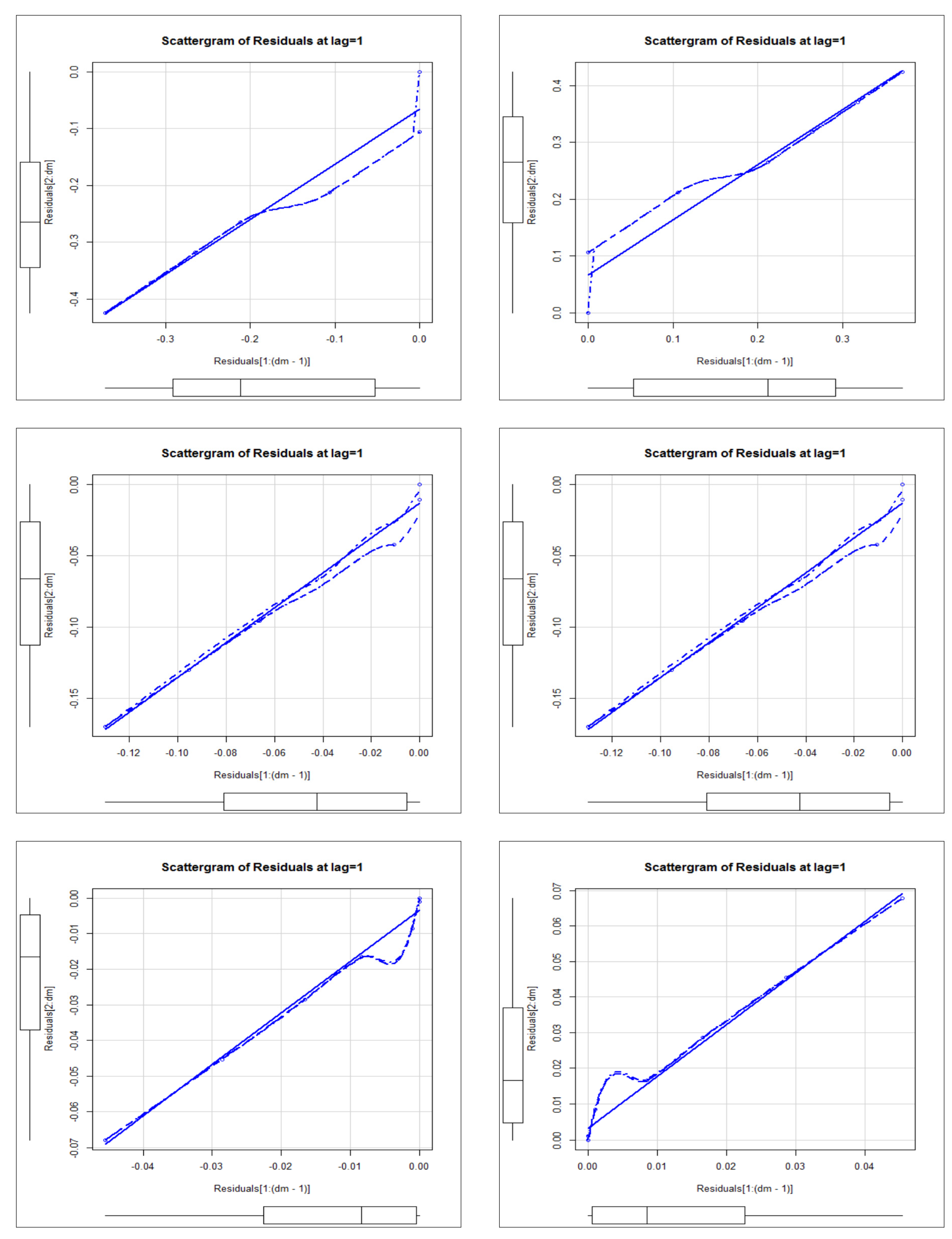
Figure 22 (first row-left panel) gives the scattergrams for the deviations under ${\phi }^{+}$ for the future value $y_{29}$. Figure 22 (first row, left panel) gives the scattergrams for the deviations for ${\phi }^{-}$ for the future value $y_{29}$. Figure 22 (second row, left panel) gives the scattergrams for the deviations under ${\phi }^{+}$ for the future value $y_{30}$. Figure 22 (second row, left panel) gives the scattergrams for the deviations for ${\phi }^{-}$ for the future value $y_{30}$. Figure 22 (third row, left panel) gives the scattergrams for the deviations under ${\phi }^{+}$ for the future value $y_{31}$. Figure 22 (third row, left panel) gives the scattergrams for the deviations for ${\phi }^{-}$ for the future value $y_{31}$. Figure 22 (first row) gives the deviations, absolute deviations and square deviations against ${\phi }^{+}$ (the future value $y_{29}$ (left), the future value $y_{30}$ (middle) and the future value $y_{31}$ right)). Figure 16 (second row) gives the deviations, absolute deviations and square deviations against ${\phi }^{-}$ (the future value $y_{29}$ (left), the future value $y_{30}$ (middel) and the future value $y_{31}$ right)). Figure 23 gives the deviations, absolute deviations and square deviations for ${\phi }^{+}$ (((a),(b),(c))) and ${\phi }^{-}$ ((d),(e),(f)).

7.2. An Application for Risk Analysis under the Insurance-Claims Payment Data

In this subsection, we present an application for risk analysis under the VaR, TVaR, TV and TMV measures presented in (13), (15), (16) and (17) using the insurance-claims payment data. The risk analysis is performed using some confidence levels ($\epsilon = 70\%,75\%,80\%,85\%,90\%,95\%,99\%$). The four measures are estimates for the EWC and the MOGC models.

The MOGC model is considered the best competitive model. Table 8 below gives the RIs for the EWC the MOGC models. For the EWC model, the VaR$\epsilon$ for EWC ranges from 9.003261 to 11.999004, the TVaR$\epsilon$ for EWC ranges from 11.999302 to 14.00635, the TV$\epsilon$ for EWC ranges from 2.008071 to 2.9989921 and the TMV$\epsilon$ for EWC ranges from 12.190242 to 16.450089. The VaR$\epsilon$ for MOGC ranges from 6.004395 to 9.642490, the TVaR$\epsilon$ for MOGC ranges from 6.721463 to 9.909357, the TV$\epsilon$ for MOGC ranges from 1.011332 to 2.102319 and the TMV$\epsilon$ MOGC ranges from 6.961463 to 12.909357. The following conclusion can be summarized:

• VaR$\epsilon$ for EWC > VaR$\epsilon$ for MOGC and TVaR$\epsilon$ for EWC > TVaR$\epsilon$ for MOGC.
• TV$\epsilon$ for EWC > TV$\epsilon$ for MOGC and TMV$\epsilon$ for EWC > TMV$\epsilon$ for MOGC.
• VaR$\epsilon$(X) < TVaR$\epsilon$(X) < TMV$\epsilon$(X) $\forall$ $\epsilon$.

8. Conclusions

A novel, flexible extension of the Chen distribution that accommodates “decreasing–constant–increasing (bathtub)”, “monotonically increasing”, “upside down constant–increasing”, “monotonically decreasing”, “J” and “upside down” failure rates was defined and studied. The new model was motivated by its wide applicability in modeling “unimodal right-skewed”, “unimodal left-skewed”, “bimodal right-skewed” and “bimodal left-skewed” real data. Relevant statistical properties of the novel model were derived such as conditional moments, mean residual life and mean past lifetime. The method of maximum likelihood estimation was considered for estimating the model parameters. In the medical field, the proposed distribution was used for modeling data on the relief times of patients, which was characterized as being asymmetric bimodal with a right tail and has one extreme observation. Many risk indicators were considered and studied such as the value at risk, the tail value at risk (conditional tail expectation), the conditional value at risk, the tail variance and the tail mean variance. The four indicators were applied and the data on insurance-claims payments were negatively skewed. Since the insurance-claims data were a quarterly time series, we analyzed it using the AR(1) model. The autocorrelation function and the partial autocorrelation function plots were presented. The AR(1) model was suggested for obtaining the future values $y_{29}$ (2014 first quarter) with $\phi = {10}^{-7}$ or $\phi = -{10}^{-7}$ since deviation = absolute deviation = square deviation $\cong 0$. The AR(1) model was suggested for obtaining the future values $y_{30}$ (2014 s quarter) with $\phi = \pm {10}^{-7}$ or $\phi = \pm {10}^{-4}$ since deviation = absolute deviation = square deviation $\cong 0$. The AR(1) model was suggested for obtaining the future values $y_{31}$ ((2014 third quarter)) with $\phi = \pm {10}^{-7}$ or $\phi = \pm {10}^{-4}$ since deviation = absolute deviation = square deviation $\cong 0$.

The new model has multiple applications in the field of statistical modeling and forecasting, as illustrated below:

• In the medical field, the EWC distribution can be used to model the data on patient’s relief times, which is characterized as being asymmetric bimodal with a right tail and has one extreme observation. Although there are many competing distributions in the field of statistical modeling in the medical field such as Gamma-Chen distribution, Kumaraswamy Chen distribution, Beta-Chen distribution, Marshall–Olkin Chen distribution, Transmuted Chen distribution and standard two-parameter Chen distribution, the EWC distribution proved its superiority in the statistical modeling of the data on relief times with minimum values for the Akaike Information Criteria, the Bayesian Information Criteria, the Cramér–Von Mises test, the Anderson–Darling test, Kolmogorov–Smirnov test and their corresponding p-values.
• In the field of planning and management of the use of water resources, we modeled the lower discharge of at least seven consecutive days and return period (time) of ten years for the Cuiaba River, Cuiaba, Mato Grosso, Brazil over 38 years using the EWC distribution. These data were characterized as being asymmetric and bimodal. Although there are many competing distributions in the field of statistical modeling for data in the planning and management of the use of water resources such as Gamma-Chen distribution, Kumaraswamy Chen distribution, Beta-Chen distribution, Marshall–Olkin Chen distribution, Transmuted Chen distribution, Transmuted exponentiated Chen distribution and standard two-parameter Chen distribution, the EWC distribution proved its superiority in statistical modeling for data in the planning and management of the use of water resources with minimum values for the Akaike Information Criteria, the Consistent Information Criteria, the Bayesian Information Criteria, the Hannan–Quinn Information Criteria, the Cramér–Von Mises, the Anderson–Darling test, the Kolmogorov–Smirnov (K.S) test and their corresponding p-value.
• In the insurance and actuarial science field, we analyzed the insurance-claims payment triangle from a U.K. motor non-comprehensive account using the EWC distribution. These data were characterized as being asymmetric bimodal and negatively skewed. Although there are many competing distributions in the field of statistical modeling for data in insurance and actuarial sciences such as standard exponential distribution, standard Chen distribution, Rayleigh Chen distribution, exponential Chen distribution, Marshall–Olkin generalized Chen distribution, reduced Burr X Chen distribution, Weibull Chen distribution, Lomax Chen distribution, standard exponentiated distribution, Burr X exponentiated Chen distribution, Burr XII Chen distribution and Log logistic Chen distribution, the EWC distribution proved its superiority in statistical modeling for data in insurance and actuarial science with minimum values for the Akaike Information Criteria, the Bayesian Information Criteria, the Cramér–Von Mises test, the Anderson–Darling test, the Kolmogorov–Smirnov test and their corresponding p-value.
• The HRF of the new Chen extension can be “decreasing–constant–increasing (bathtub)”, “monotonically increasing”, “upside down constant–increasing”, “monotonically decreasing”, “J shape” and “upside down”. However, the HRF function of the Chen distribution can only be “monotonically increasing” and a “bathtub (U)” shape. The density of the EWC distribution accommodates the “unimodal right-skewed”, “unimodal left-skewed”, “bimodal right-skewed” and “bimodal left-skewed” shapes. Various HRFs provide an advantage for the EWC distribution against the standard exponential distribution, standard Chen distribution, Marshall–Olkin generalized Chen distribution, Rayleigh Chen distribution, exponential Chen distribution, the standard exponentiated distribution, Burr X exponentiated Chen distribution, Burr XII Chen distribution, reduced Burr X Chen distribution, Weibull Chen distribution, Lomax Chen distribution and Log logistic Chen distribution in modeling medical data, planning and management of the use of water resource data, and insurance-claims payment triangle data.

References

- Klugman, S.A.; Panjer, H.H.; Willmot, G.E. Loss Models: From Data to Decisions; John Wiley & Sons: New York, NY, USA, 2012; Volume 715. [Google Scholar]
- Wirch, J. Raising Value at Risk. N. Am. Actuar. J. 1999, 3, 106–115. [Google Scholar] [CrossRef]
- Tasche, D. Expected Shortfall and Beyond. J. Bank. Financ. 2002, 26, 1519–1533. [Google Scholar] [CrossRef] [Green Version]
- Acerbi, C.; Tasche, D. On the coherence of expected shortfall. J. Bank. Financ. 2002, 26, 1487–1503. [Google Scholar] [CrossRef] [Green Version]
- Furman, E.; Landsman, Z. Tail variance premium with applications for elliptical portfolio of risks. ASTIN Bull. 2006, 36, 433–462. [Google Scholar] [CrossRef] [Green Version]
- Landsman, Z. On the tail mean--variance optimal portfolio selection. Insur. Math. Econ. 2010, 46, 547–553. [Google Scholar] [CrossRef]
- Artzner, P. Application of coherent risk measures to capital requirements in insurance. N. Am. Actuar. J. 1999, 3, 11–25. [Google Scholar] [CrossRef]
- Chen, Z. A new two-parameter lifetime distribution with bathtub shape or increasing failure rate function. Stat. Probab. Lett. 2000, 49, 155–161. [Google Scholar] [CrossRef]
- Cordeiro, G.M.; Afify, A.Z.; Yousof, H.M.; Pescim, R.R.; Aryal, G.R. The exponentiated Weibull-H family of distributions: Theory and Applications. Mediterr. J. Math. 2017, 14, 155. [Google Scholar] [CrossRef]
- Dey, S.; Kumar, D.; Ramos, P.L.; Louzada, F. Exponentiated Chen distribution: Properties and estimation. Commun. Stat.-Simul. Comput. 2017, 46, 8118–8139. [Google Scholar] [CrossRef]
- Aidi, K.; Butt, N.S.; Ali, M.M.; Ibrahim, M.; Yousof, H.M.; Shehata, W.A.M. A Modified Chi-square Type Test Statistic for the Double Burr X Model with Applications to Right Censored Medical and Reliability Data. Pak. J. Stat. Oper. Res. 2021, 17, 615–623. [Google Scholar] [CrossRef]
- Almazah, M.M.A.; Almuqrin, M.A.; Eliwa, M.S.; El-Morshedy, M.; Yousof, H.M. Modeling Extreme Values Utilizing an Asymmetric Probability Function. Symmetry 2021, 13, 1730. [Google Scholar] [CrossRef]
- Shehata, W.A.M.; Yousof, H.M. The four-parameter exponentiated Weibull model with Copula, properties and real data modeling. Pak. J. Stat. Oper. Res. 2021, 17, 649–667. [Google Scholar] [CrossRef]
- Yadav, A.S.; Goual, H.; Alotaibi, R.M.; Ali, M.M.; Yousof, H.M. Validation of the Topp-Leone-Lomax Model via a Modified Nikulin-Rao-Robson Goodness-of-Fit Test with Different Methods of Estimation. Symmetry 2020, 12, 57. [Google Scholar] [CrossRef] [Green Version]
- Christofides, S. Regression models based on log-incremental payments. Claims Reserving Man. 1997, 2, D5.1–D5.53. [Google Scholar]
- Cooray, K.; Ananda, M.M.A. Modeling actuarial data with a composite lognormal-Pareto model. Scand. Actuar. J. 2005, 2005, 321–334. [Google Scholar] [CrossRef]
- Lane, M.N. Pricing risk transfer transactions 1. ASTIN Bull. J. IAA 2000, 30, 259–293. [Google Scholar] [CrossRef] [Green Version]
- Bahnemann, D. Distributions for actuaries. CAS Monogr. Ser. 2015, 2, 1200. [Google Scholar]
- Embrechts, P.; Resnick, S.I.; Samorodnitsky, G. Extreme value theory as a risk management tool. N. Am. Actuar. J. 1999, 3, 30–41. [Google Scholar] [CrossRef]
- Yousof, H.M.; Al-nefaie, A.H.; Aidi, K.; Ali, M.M.; Ibrahim, M. A Modified Chi-square Type Test for Distributional Validity with Applications to Right Censored Reliability and Medical Data: A Modified Chi-square Type Test. Pak. J. Stat. Oper. Res. 2021, 17, 1113–1121. [Google Scholar] [CrossRef]
- Calderín-Ojeda, E.; Kwok, C.F. Modeling claims data with composite Stoppa models. Scand. Actuar. J. 2016, 9, 817–836. [Google Scholar] [CrossRef]
- Mansour, M.M.; Ibrahim, M.; Aidi, K.; Butt, N.S.; Ali, M.M.; Yousof, H.M.; Hamed, M.S. A new log-logistic lifetime model with mathematical properties, copula, modified goodness-of-fit test for validation and real data modeling. Mathematics 2020, 8, 1508. [Google Scholar] [CrossRef]
- Zeng, Q.; Guo, Q.; Wong, S.C.; Wen, H.; Huang, H.; Pei, X. Jointly modeling area-level crash rates by severity: A Bayesian multivariate random-parameters spatio-temporal Tobit regression. Transp. A Transp. Sci. 2019, 15, 1867–1884. [Google Scholar] [CrossRef]
- Zeng, Q.; Hao, W.; Lee, J.; Chen, F. Investigating the impacts of real-time weather conditions on freeway crash severity: A Bayesian spatial analysis. Int. J. Environ. Res. Public Health 2020, 17, 2768. [Google Scholar] [CrossRef]
- Yousof, H.M.; Ali, M.M.; Goual, H.; Ibrahim, M. A new reciprocal Rayleigh extension: Properties, copulas, different methods of estimation and modified right censored test for validation. Stat. Transit. New Ser. 2021, 23, 1–23. [Google Scholar] [CrossRef]
- Shehata, W.A.M.; Yousof, H.M.; Aboraya, M.A. Novel Generator of Continuous Probability Distributions for the Asymmetric Left-skewed Bimodal Real-life Data with Properties and Copulas. Pak. J. Stat. Oper. Res. 2021, 17, 943–961. [Google Scholar] [CrossRef]
Figure 1.
Some PDF plots for the new model, (a) unimodal right skewed with one peak, (b) reversed-J PDF, (c) one peak unimodal right skewed, (d) bimodal right skewed with heavy tail, (e) bimodal right skewed and (f) unimodal left skewed, bimodal right skewed.
Figure 2.
Some HRF plots for the new model, (a) monotonically increasing, (b) monotonically decreasing, (c) increasing- constant– increasing, (d) decreasing–constant–increasing (bathtub)”, (e) upside down constant–increasing and (f) constant.
Figure 3.
Rényi entropy index for the EWC model for some selected parameters value, (a) , (b) , (c) , (d) .
Figure 4.
Box plots.
Figure 5.
Q–Q plots.
Figure 6.
TTT plots.
Figure 7.
NKDE plots.
Figure 8.
(a) P–P, (b) E-PDF, (c) E-HRF and (d) Kaplan–Meier plots for the data on relief times.
Figure 9.
(a) P–P, (b) E-PDF, (c) E-HRF and (d) Kaplan–Meier plot for the minimum flow data.
Figure 10.
(a) NKDE, (b) Q–Q, (c) TTT and (d) box plots for raw claims data.
Figure 11.
Describing the insurance-claims data, (a) Scattergram with no line, (b) Smoothed Scattergram, (c) Standard Scattergram, (d) Cullen–Frey plot (e) ACF plot and (f) partial ACF plot for insurance-claims data.
Figure 12.
E-PDF, E-HRF and KM plots for insurance-claims data.
Figure 13.
P–P plots for some competitive models.
Figure 14.
Artificial claims with ACF and partial ACF for and .
Figure 15.
Figure 16.
Figure 17.
Figure 18.
Figure 19.
Figure 20.
Figure 21.
Figure 22.
Scattergrams for the deviations.
Figure 23.
(a) Deviations, absolute deviations and square deviations for , (b) Deviations, absolute deviations and square deviations for , (c) Deviations, absolute deviations and square deviations for , (d) Deviations, absolute deviations and square deviations for , (e) Deviations, absolute deviations and square deviations for , (f) Deviations, absolute deviations and square deviations for .