Estimating the Reattachment Length by Realizing a Comparison between URANS k-Omega SST and LES WALE Models on a Symmetric Geometry

Abstract

In this study, a water reattachment length was calculated by adopting two different models. The first was based on Unsteady Reynolds-Averaged Navier–Stokes (URANS) k-omega with Shear Stress Transport (SST); the second was a Large Eddy Simulation (LES) with Wall-Adapting Local Eddy-Viscosity (WALE). Both models used the same mesh and were checked with Taylor length-scale analysis. After the analysis, the mesh had 11,040,000 hexahedral cells. The geometry was a symmetrical expansion–contraction tube with a 4.28 expansion ratio that created mechanical energy losses, which were taken into account. Moreover, the reattachment length was estimated by analyzing the speed values; the change of speed value from negative to positive was used as the criterion to recognize the reattachment point.

1. Introduction

Particle Image Velocimetry (PIV) is a conventional method of visualizing optical flow [1]. It consists of obtaining instantaneous velocity measurements and related properties in fluids that have to be illuminated so that the particles can be seen. Hence, an experimental test area cannot be a traditional opaque pipeline [2]. A similar method known as Particle Tracking Velocimetry (PTV) determines the velocity of particles in a moving fluid [3]. The difference is that PIV analyzes the mean displacement of small particles, whereas PTV tracks the motion of individual particles. The details obtained from the PTV are the characterization of the particle size, such as the mean particle diameter (in pixels and mm), standard deviation, and the total number of particles detected [4].

PIV and PTV can be used to analyze particle behavior with different retention systems. The most conventional technique for particle collection is sedimentation, in which fluid velocity is reduced to the falling of particles because of gravity [5,6]. Another common technique is to use a membrane as a filter to prevent particle circulation without affecting the fluid flow [7,8]. In case the particles have a metallic component, a magnetic force can be established in the pipeline [9,10].

To realize a sedimentation retention pipeline, the hydraulic diameter of the pipe must be increased to reduce fluid velocity. This change in diameter alters the fluid behavior, which is known as the reattachment length. This phenomenon depends on sudden expansion and was demonstrated by Kuehn [11] in 1980. Despite implementing a high aspect ratio in the test area, the flow maintained a bidimensional behavior downstream the step for all Reynolds numbers (see the study of Armaly et al. [12]).

Nevertheless, more recent studies showed that the reattachment length depends on geometric design, expansion ratio, inlet and outlet conditions, and turbulence intensity, as well as heat transfer conditions [13].

The reattachment length and flow separation are common in internal flow diffusers, turbines, combustors, and buildings [14]. To estimate the reattachment length, the most common technique is to validate the simulation by adopting PIV techniques [15]. However, theoretical investigation based on numerical simulation can be performed [16], which is most common design process.

Therefore, the estimation can be performed by adopting one of four different experiments [17]. The first consists of analyzing the average velocity near the wall. When the velocity changes from negative to positive, the reattachment length will be established. The second evaluates the wall-shear stress and locates the areas with zero values. The third locates the mean dividing streamline. The last one indicates the location of 50% of the forward flow fraction. In addition, a correlation derived experimentally states that the reattachment can be $X_r=6.28·h$ for a low Reynolds number, considering $h$ as the step length. This affirmation can also be proven by the experiment of So et al. [18].

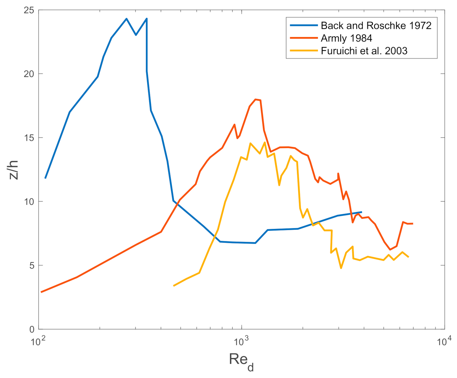
Nie and Armaly [19] presented a scheme for a specific step–wall ratio that estimates the location where the shear stress is zero as a function of different Reynolds numbers. Moreover, Furuichi et al. [20] showed a comparison among the results of two other studies (see Figure 1).

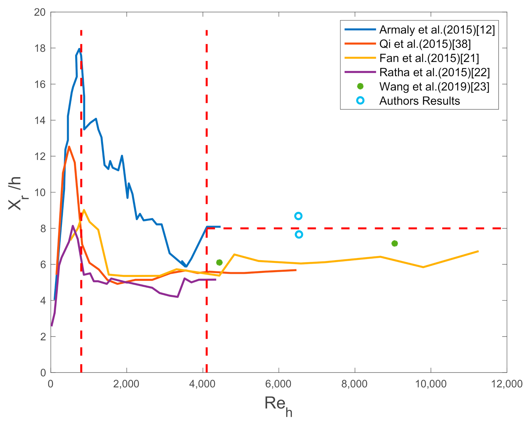
Figure 1 1is being updated by PIV experiments, such as those by Fan et al. [21] and Ratha and Sarkar [22]. On the one hand, in the first of these works, the researchers analyzed the reattachment length with different Reynolds (Re) numbers ranging from 500 to 50,000. The results revealed that the reattachment zone increased with the increase in Re when it was less than 840. The length of the reattachment ($X_r$) decreased with the increase in Re in the case of 840 < Re < 1642. The length of $X_r$ increased slowly in the case of 1642 < Re < 4800. Then the length stabilized when 4800 < Re < 15,523.

On the other hand, in the second of these works, the authors experimented with other Re values and also with different expansion ratios. Additionally, Wang et al. [23] presented other experimental results to review the differences between the values of Fan et al. [21] and each value.

The aim of this article is to locate the reattachment length of a specific geometry. For this purpose, two different types of simulations with the same conditions are compared. The first one uses LES WALE-based models, and the second one uses k-omega SST. The mesh is validated by performing various analyses, such as Face Validity. In addition, the Taylor length scale is calculated to verify sufficient cell resolution.

2. Materials and Methods

This section is divided into three subsections. In the first, the problems of reattachment are presented along with a particular geometry. In the second, the physics of the simulations are explained. Finally, the development and validation of the mesh is discussed. The symbols used in the current work are presented in the Abbreviations section.

2.1. Problem of Description and Geometry Design

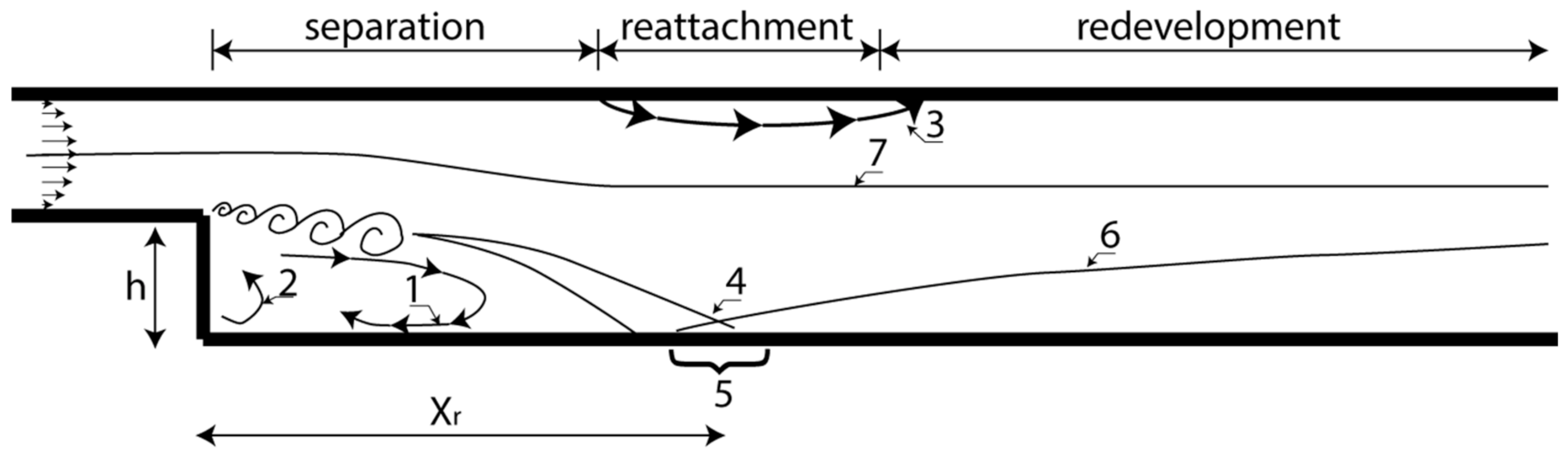
Estimation of the reattachment position after flow separation is a well-known problem that can be faced by evaluating different physical parameters. Conventional estimations are based on an analysis of the average velocity near the wall, which changes from a negative to a positive value when passing through the reattachment position [24]. Due to the sudden expansion of the pipe diameter, the flow does not follow the trend curve in the wider pipe. As a result, flow separation occurs, creating recirculation zones where the pipe expands (Figure 2). To avoid the reattachment phenomenon, a particular ramp could be appropriately designed to avoid a high-value reattachment length.

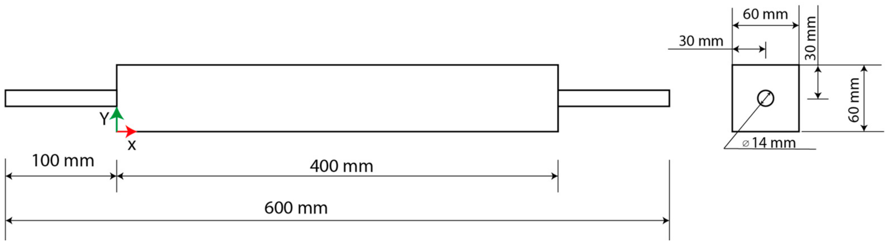
In contrast to Figure 2 a symmetrical geometry was used in the current work. The particular design is depicted in Figure 3. The water inlet and outlet were 14 mm diameter pipes. Nevertheless, the test area was a rectangular geometry of 60 × 60 × 400 mm. The simulation setup was designed as three-dimensional to achieve a better resolution [25].

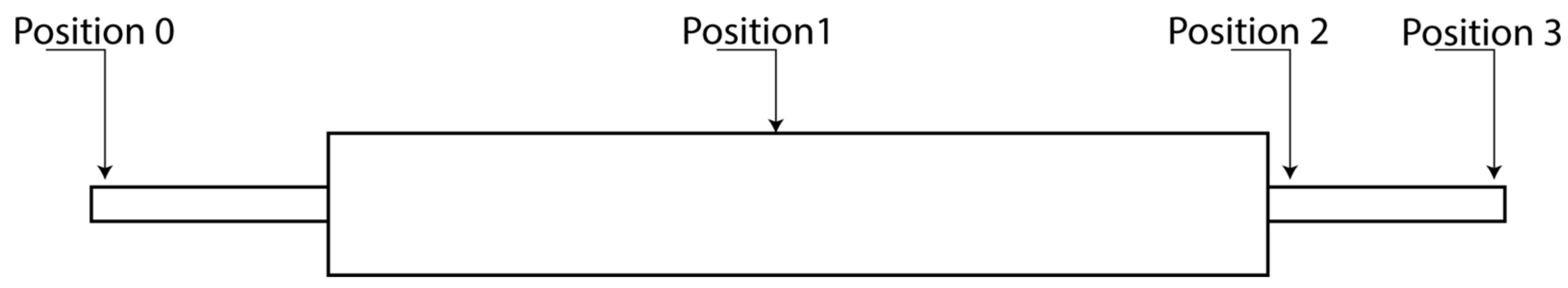
Due to the design, there were mechanical losses. Sudden expansions and contractions affected the conservation of energy and had to be estimated for the design of an installation. To evaluate the mechanical losses, Chanson [26] proposed Borda–Carnot equations (see Equations (1)–(6) below); Figure 4 shows the evaluation points in the particular geometry.

$$∆E_{expansion}=\frac{\epsilon }{2}·\rho ·{\left(v_0-v_1\right)}^2=\frac{1}{2}·\rho ·{\left(\frac{1}{\mu }-1\right)}^2·{\left(\frac{A_0}{A_1}\right)}^2·U_0^2$$

(1)

$$∆H=\frac{∆E_{expansion}}{\rho ·g}=\frac{1}{2g}·{\left(1-\frac{A_0}{A_1}\right)}^2·U_0^2$$

(2)

$$∆p=p_0-p_1=-\rho ·\frac{A_0}{A_1}·\left(1-\frac{A_0}{A_1}\right)·U_0^2$$

(3)

$$∆h=h_0-h_1=-\frac{1}{g}·\frac{A_0}{A_1}·\left(1-\frac{A_0}{A_1}\right)·U_0^2$$

(4)

$$∆E_{contraction}=\frac{1}{2}·\rho ·{\left(U_2-U_3\right)}^2=\frac{1}{2}· \rho ·{\left(\frac{1}{{\mu }_{loss}}-1\right)}^2·{\left(\frac{A_1}{A_3}\right)}^2·U_1^2$$

(5)

$${\mu }_{loss}=0.63+0.37·{\left(\frac{A_3}{A_1}\right)}^3$$

(6)

Equations (1) and (5) are the Borda–Carnot equations that estimate mechanical energy loss. Equation (2) calculates total head loss. Equation (3) represents the total kinetic energy change between the two cross-sections, and the loss coefficient (ξ) for this sudden expansion is approximately equal to one. Equation (4) shows the variation of the hydraulic head. Finally, Equation (6) agrees with the measurements of Oertel et al. [27], in which it is an approximation of the shrinkage coefficient for a sharp-edged shrinkage. The results of these equations are represented in

Table 1. The constants and mechanical loss.

Property	Values
$\mathrm{Density}(\rho )$	$997.561\mathrm{kg}/{\mathrm{m}}^3$
Dynamic viscosity ($\mu$)	$8.8871·{10}^{-4}\mathrm{Pa}·\mathrm{s}$
$\mathrm{Pipeline}\mathrm{diameter}\left(D\right)$	0.014 m
Loss coefficient (ξ)	1
Step (h)	0.023 m
$A_0=A_2=A_3$	$0.000154{\mathrm{m}}^2$
$A_1$	$0.0036{\mathrm{m}}^2$
g	$9.18\mathrm{m}/{\mathrm{s}}^2$
$U_0=U_2=U_3$	$1\mathrm{m}/\mathrm{s}$
$U_1$	$0.0427\mathrm{m}/\mathrm{s}$
$∆E_{expansion}$	$457.04\mathrm{J}/{\mathrm{m}}^3$
$∆H$	$0.047$
$∆p$	$-40.83\mathrm{Pa}$
$∆h$	$-0.0041\mathrm{m}$
$∆E_{contraction}$	$171.99\mathrm{J}/{\mathrm{m}}^3$
${\mu }_{loss}$	$0.63$

.

2.2. Simulation Physics

To achieve the objective of this study, two methods were considered. The first was based on a Large Eddy Simulation (LES) [28]. Choi et al. [29] calculated an empirical model to estimate a consistent LES architecture, in which a more accurate formula for the boundary layer flow at a high Reynolds number was used to suggest new grid-point requirements for a wall-modeled and wall-resolving LES.

According to Portal-Porras et al. [30], the LES-based technique provided better resolution per cell than conventional ones did. The LES is a mathematical turbulence model used in computational fluid dynamics [31,32]. The main idea is to reduce computational costs relative to direct numerical simulation (DNS) via low-pass filtering of the Navier–Stokes equations to model the smallest-length scales, the most computationally expensive to resolve [33]. To model the physics in these cells, the Wall-Adapting Local Eddy-Viscosity (WALE) subgrid scale (SGS) model was selected.

Numerical simulations performed with the LES agreed with the experimental results, which showed it to be suitable for predicting the effect of pipe wall corrugation on the mean flow in a range of Reynolds numbers typical of engineering applications [34].

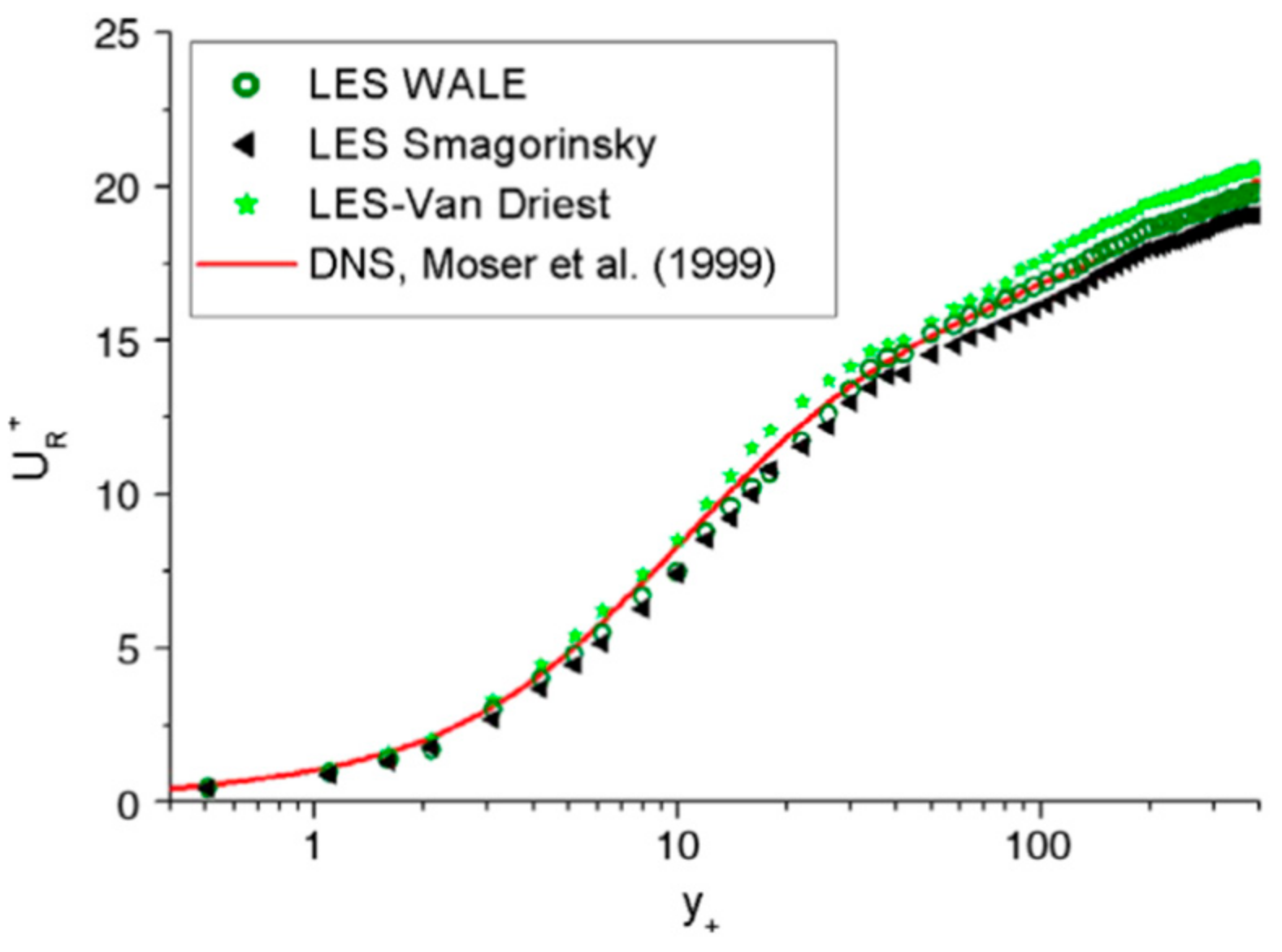
The LES model led to some improvements, and Weickert et al. [35] analyzed the differences among the LES WALE, LES–Smagorinsky, and LES–Van Driest models with respect to the DNS.

Figure 5 illustrates the behavior of the averaged dimensionless velocity $u_{+}$ versus the dimensionless wall distance $y_{+}$ for the finest grid resolution. Since the WALE model gave the correct near-wall scaling of $y_{+}^3$, the obtained data set corresponded to Moser’s DNS data. Smagorinsky’s model and the LES–Van Driest model differed significantly from the DNS simulation. One reason for this is that the near-wall scaling had not been correctly reproduced. Specifically, the Smagorinsky model had a near-wall scaling of $y_{+}$, whereas the LES–Van Driest models had a near-wall scaling of $y_{+}^2$. Therefore, the LES WALE model provided a better perform.

The other technique is the conventional Reynolds-Averaged Navier–Stokes (RANS) [36] applied to an unsteady-state flow. According to Tomboulides et al. [37], the RANS approach needs to track the evolution of the spatial and temporal scales. Quantities such as velocity are assumed to comprise mean and fluctuating components. Therefore, time-dependent Navier–Stokes (NS) equations are used to obtain the unsteady RANS equations (URANS). Maliska et al. [38] presented a comparison of Large Eddy Simulation and Scale Adaptative Simulation versus k-omega shear stress transport (SST) models, based on the URANS model, which presented consistent results when average quantities were compared. Moreover, Khalili et al. [39] compared URANS, LES, and Detached Eddy Simulation (DES) with the experimental measurements, and the LES model showed better agreement with the velocity measurements. Moreover, the k-omega SST model uses the low-y^+ formulation, which resolves the viscous sublayer and needs little or no modeling to predict the flow across the wall boundary, and if the cell height is in the log-law layer, it uses the wall function. On the other hand, LES WALE uses the all-y^+ formulation, which emulates the low-y^+ wall treatment for fine meshes (near the boundaries); and the high-y^+ wall treatment for coarse meshes (far from the boundaries), which instead of resolving the viscous sublayer, obtains the boundary conditions for the continuum equations.

First, in the present work, URANS-based numerical simulations in combination with Menter’s k-omega SST [40] for turbulence modelling were performed. The time step (Δt) of the simulations was set to 0.0005 s, and the inner iterations were 12, which meant that the Courant–Friederichs–Levy (CFL) number was equal to 0.5 according to Expression (7); therefore, the CFL condition (CFL < 1) was fulfilled. Second, LES simulations were run with the SGS and WALE models.

$$\mathrm{CFL}=\frac{u_{\infty }·∆t}{∆x}$$

(7)

where $∆x$ is the smallest cell length in the direction of the flow. The fluid in the study, water had a constant density of $997.561\mathrm{kg}/{\mathrm{m}}^3$ and a dynamic viscosity of $8.8871·{10}^{-4}\mathrm{Pa}·\mathrm{s}$ at a temperature of 20 °C. In addition, gravity affecting the y axis with a value of $-9.98 \mathrm{m}/{\mathrm{s}}^2$ was considered.

The velocity at the inlet condition of the liquid was $U_0=1\raisebox{1ex}{$\mathrm{m}$}\!\left/ \!\raisebox{-1ex}{$\mathrm{s}$}\right.$. Therefore, the Reynolds number in the pipeline was 13,930.21. Adopting the Bernoulli rule, where the flow remains constant, the Re in the testing area (60 × 60 × 400 mm area) was 5105.69 (see Equation (8)). Since the test area was rectangular, a hydraulic diameter had to be considered, which was governed by Equation (8). Table 1 shows the values of the constants used in Equations (8) and (9).

$$D_h=\frac{4·A_1}{Perimeter}=\frac{4·0.0036 {\mathrm{m}}^2}{4·0.06}=0.06 \mathrm{m}$$

(8)

$$R{e}_{pipe}=\frac{\rho ·U_0·D}{\mu }=13,930.21\hspace{1em}R{e}_{testing\_area}=\frac{\rho ·U_1·D_h}{\mu }=5105.69$$

(9)

A 16-core Intel i7 with 32 GB of RAM was used to obtain the simulation results. Star CCM+ software was selected to process the values. Depending on the stopping criterion, the time duration differed. In the current work, the maximum physical time was set at 2 s; thus, the k-omega SST model needed about 48 h to complete the simulation, and the LES WALE model about 144 h.

2.3. Mesh Development and Validation

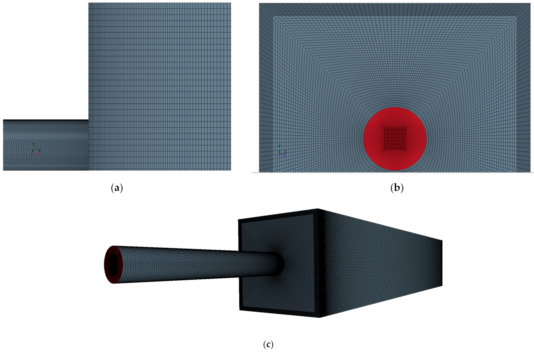
The next step was to create the mesh. On this occasion, both simulations had the same number of cells to compare the k-omega SST with LES WALE. The hexahedral cells number was 11,040,000, and Figure 6 shows the mesh from different perspectives.

Table 2. The results of the mesh metrics.

Mesh Property	Value	Well Perform Criteria
Face Validity	0.95	>0.5
Minimum Cell Quality	0.175042	>1 × 10−5
Minimum Volume Change	0.2158	>0.01
Minimum Least Squares Quality	0.113789	>0.001
Minimum Cell Warpage Quality	1	>0.15
Maximum Skewness Angle	124.829 °	0.0° < skewness angle < 75°

shows the results of the mesh metrics.

To verify the quality of the mesh and cells, Budd et al. [41] presented analyses of the cell skewness angle and cell quality. In the following lines, the working mesh in this study was evaluated to assess its performance, if the mesh performed well. The parameters and conditions evaluated to determine a good mesh are presented in [42].

The first item was the Face Validity, a subjective measure of the correctness of the face-normal relative to its attached cell centroid [43]. The mesh had a Face Validity value of 0.95 for most of the cells. However, four cells had a value of 0.999995. Even with these four cells, the mesh had a positive value, which means that the Face Validity was higher than 0.5.

The Cell Quality metric algorithm is based on a hybrid approach using the Gauss and least squares methods for cell gradient calculation; it utilizes a function that considers a relative geometric distribution of the cell centroids of the facing neighbor cells and the orientation of the cell faces. For the current work, the minimum value of cell quality was 0.175. If it were less than 1 × 10⁻⁵, the mesh could be considered bad.

Another parameter was the Volume Change metric, which describes the ratio of the volume of one cell to the larger neighbor cell volume. The analysis concluded that the volume change was 0.2158, which was far from 0.01. In case the value was 0.01, the mesh had to be modified to increase the metric.

The Least Squares Quality was used to interpret cell quality. This parameter was calculated by taking the physical location of the cell centroid relative to the face-neighbor’s cell centroid. If the value were below 0.001, the cell quality was poor. Moreover, in case of LES, the quality of cell warping had to be checked. This type of cell could cause problems for the flow solver and be considered as low-quality cell, if its value was lower than 0.15.

The skewness angle is the angle between a face normal vector and the vector connecting the centroids of a cell and its neighbor cells. If the value is greater than 90° in most cells, convergence problems will occur. In the case of the current mesh, the cell skewness angle could be considered correct, as almost all cells were set below 90°. Nevertheless, there were 10 cells that had an angle of 124.829°. Thus, the percentage of wrong cells was too low to discard this mesh, considering that in the whole geometry, there were 11,040,000 cells, and the rest of the values were between 0.0 and 75°.

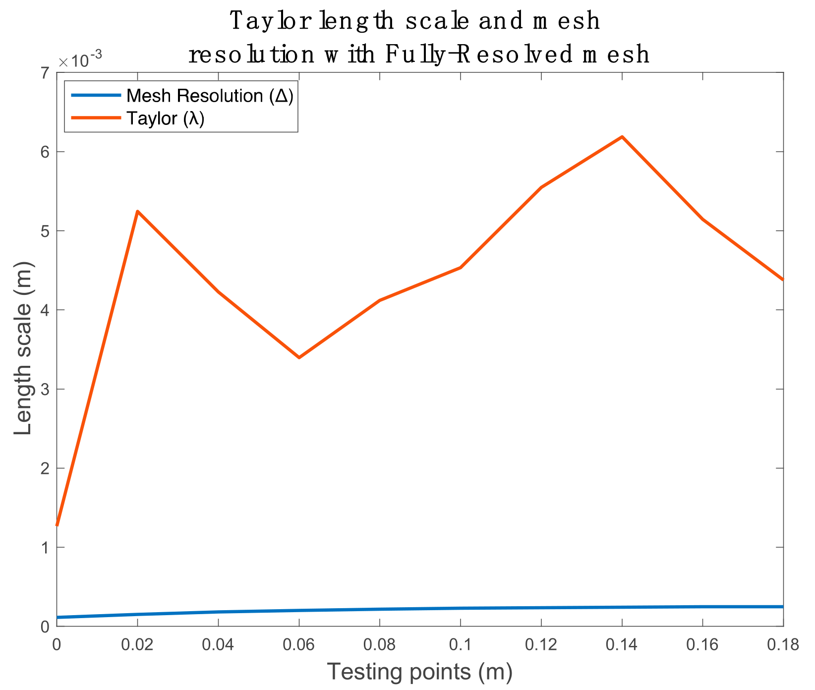
After evaluating these parameters, the LES required another evaluation to determine if the mesh had sufficient cell resolution. Hence, Portal-Porras et al. [30] mentioned that the LES mesh could be evaluated using the Taylor length scale $\left(\lambda \right)$. The experiment required evaluating the value of the mean velocity of some cells, which were close to the sudden expansion. Hence, the mesh validation can be seen in Figure 7, where the evaluating points are set at the center of the rectangle and distributed around the x axis. The first point is located right at the sudden expansion, and then nine more at 0.02 m intervals.

The mesh resolution was obtained by $∆=\sqrt[3]{V_{cell}}$. The Taylor length scale was calculated to obtain the autocorrelation function from the Taylor expansion coefficient. Then, the Taylor time scale had to be calculated. Finally, $\lambda$ was estimated from the Taylor hypothesis [44].

The experiment found a good mesh performance, as the value per point was lower than Taylor length scale, and according to the criteria of Kuczaj et al. [45], the LES mesh was validated.

3. Results

In order to make comparisons between the LES WALE and k-omega SST models, an average velocity monitoring procedure was utilized; this calculated the mean velocity of all cells during 2 s of simulation after the flow was fully developed. Thus, LES WALE could be compared with URANS k-omega SST.

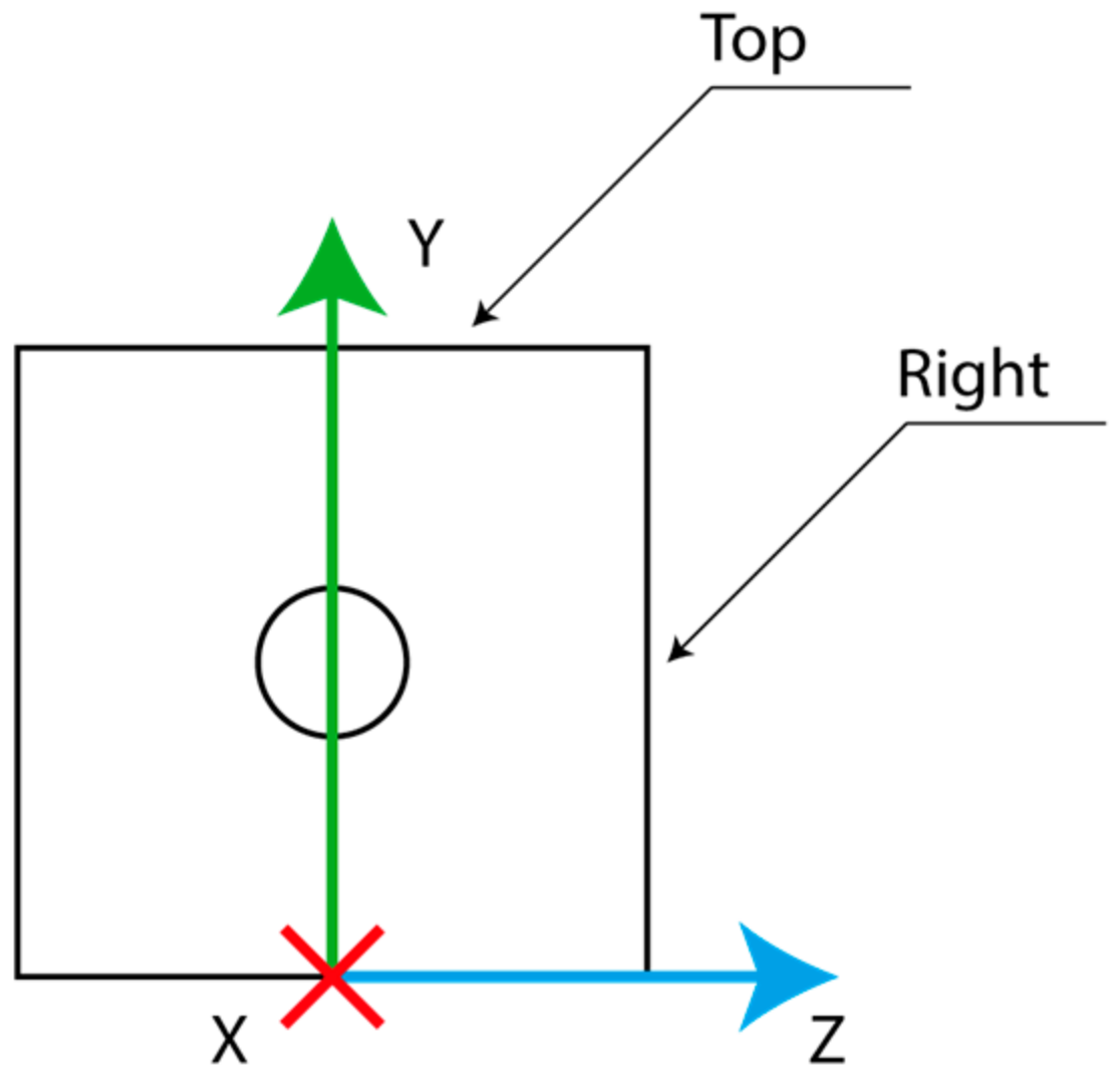
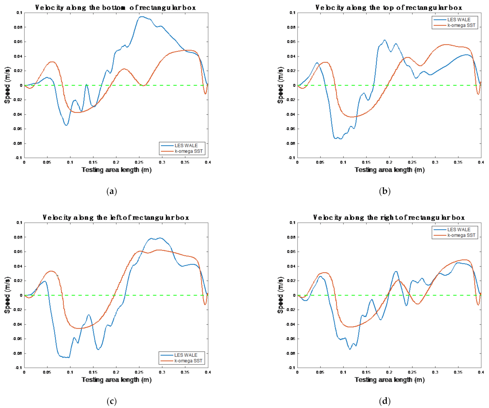
The velocity variation is used to estimate the reattachment length. For this purpose, four lines of 400 mm length were settled along the 60 × 60 × 400 mm box. They were located in the center, top, bottom, right, and left of the rectangle; that is, along x-axis at the symmetry line of the corresponding plan (see Figure 8).

In Figure 9, the velocity variations in different planes (top, bottom, left, and right) are represented. In all illustrations, there is a green line that differentiates the negative values from the positives ones. As a general conclusion, the velocity predicted by the LES WALE model exhibited more variation. Therefore, a more thorough analysis of the velocity was required.

Furthermore, around the $0.35 \mathrm{m}$ position, the flow began to show reduced velocity in all planes, and at one point had a negative value. This behavior was a consequence of the diameter reduction. For this particular case, the geometry had an expansion zone and a reduction zone. Hence, there was a vortex at the end of the test area around the $0.37 \mathrm{m}$ position. This vortex was not analyzed because the aim of this work was to find the reattachment point by analyzing velocity.

In the bottom line results, the k-omega SST reattachment length was estimated to be $0.189 \mathrm{m}$ (see Figure 9a). After this position, there was another vortex. Nevertheless, it could not be considered large, because each maximum velocity was –0.00019 m/s. Thus, this speed was negligible and could be considered zero. The bottom line revealed that the speed had more dumping behavior after the reattachment point (see Figure 9a). This phenomenon could be attributed to gravity.

The reattachment length in the LES WALE was found at $Xr=0.168 \mathrm{m}$ (see Figure 9a). It was slightly more difficult to identify, but after analyzing the whole speed evolution, there was a 0.021 m difference between the models. Moreover, gravity behaved differently in each case: the LES WALE had no negative velocity downstream of the reattachment, unlike k-omega. It also had the highest positive velocity after the reattachment length in comparison with LES results on the other three wall sides.

In Figure 9b, the top line speed variation is represented. In the k-omega SST, the reattachment point was at $0.196 \mathrm{m}$, a difference of 0.0013 m when compared to the k-omega SST at the bottom plane. However, the LES WALE differed more from the k-omega SST: its reattachment length was around $Xr=0.164 \mathrm{m}$, which was 0.03 m less.

On the left plane (Figure 9c), the reattachment length was about $0.196 \mathrm{m}$ for the k-omega SST model, which was the same value as that of the top plane (Figure 9b). Moreover, the LES WALE result (0.217 m) was similar. This value differed more from the other reattachment values. This phenomenon could be attributed to a vortex due to vortex expansion.

Finally, on the right plane (Figure 9d), the k-omega SST model had a high-speed variation from negative to positive values. The velocity became zero at 0.196 m, which was the same as that of the top plane. Nevertheless, from $0.246\mathrm{m}$ to $0.277\mathrm{m}$, the speed became negative again. In that area, the maximum negative speed was $-0.01216\mathrm{m}/\mathrm{s}$. This speed was four times less than the top minimum speed on that plane; hence, that speed could be discarded. This statement was confirmed by comparing the maximum values of negative speeds, which are displayed in

Table 3. The line results at different locations.

Property	Top Plane	Bottom Plane	Left Plane	Right Plane
k-omega SST reattachment length location $\left(X_r\right)$(m)	0.196	0.189	0.196	0.196
k-omega SST top negative speed (m/s)	−0.0435	−0.0375	−0.0458	−0.0437
LES WALE reattachment length location $\left(X_r\right)$(m)	0.164	0.168	0.217	0.194
LES WALE top negative speed (m/s)	−0.0779	−0.0609	−0.0912	−0.0857

. In the LES WALE model, the same tendency was maintained: the speed became slightly negative, but it was negligible, and the reattachment length was 0.194 m. Therefore, the reattachment point in the LES WALE could be considered to be around 0.18 m, which was the median among all the values.

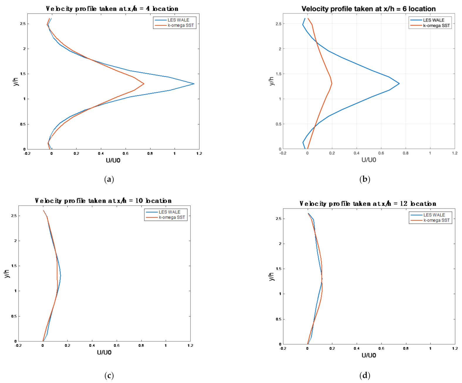
In addition to these lines, which analyzed all four planes to estimate the reattachment length, other speed measurements were taken at specific positions: x/h = 4, 6, 10, 12 [32], where x is a given position of the length of testing area after the step, and h is the length of the sudden expansion step.

Figure 10 shows the different velocity profiles taken as specific points. Moreover, the profiles were evaluated from the lower to the upper plane. In general, all cases had the same behavior, and the two models did not differ very much from each other.

The x/h = 4 position was the only one where the difference was larger (see Figure 10a). This position was close to the expansion zone, where the turbulence was highest. The maximum value of difference was approximately U/U₀ = 0.402 at the height y/h = 1.3. Therefore, the LES WALE processed a much higher turbulence than the k-omega SST did.

Flow separation is clearly represented at x/h = 4 and x/h = 6, where the speed near the wall is negative (Figure 10a,b). It is slightly difficult to see the negative values in the k-omega SST results in Figure 10b; however, after analyzing the numerical values, the statement could be confirmed.

The flow separation disappeared between the x/h = 6 and x/h = 10, as the velocity was no longer negative (cf. Figure 10b,c). Thus, it can be stated that the reattachment point will be between 0.138 and 0.23 m. The previous results fixed the reattachment at $Xr=0.196 \mathrm{m}$. In addition, the behavior of both models was practically identical for x/h = 10, which is why in some situations, the blue line is not visible in Figure 10c.

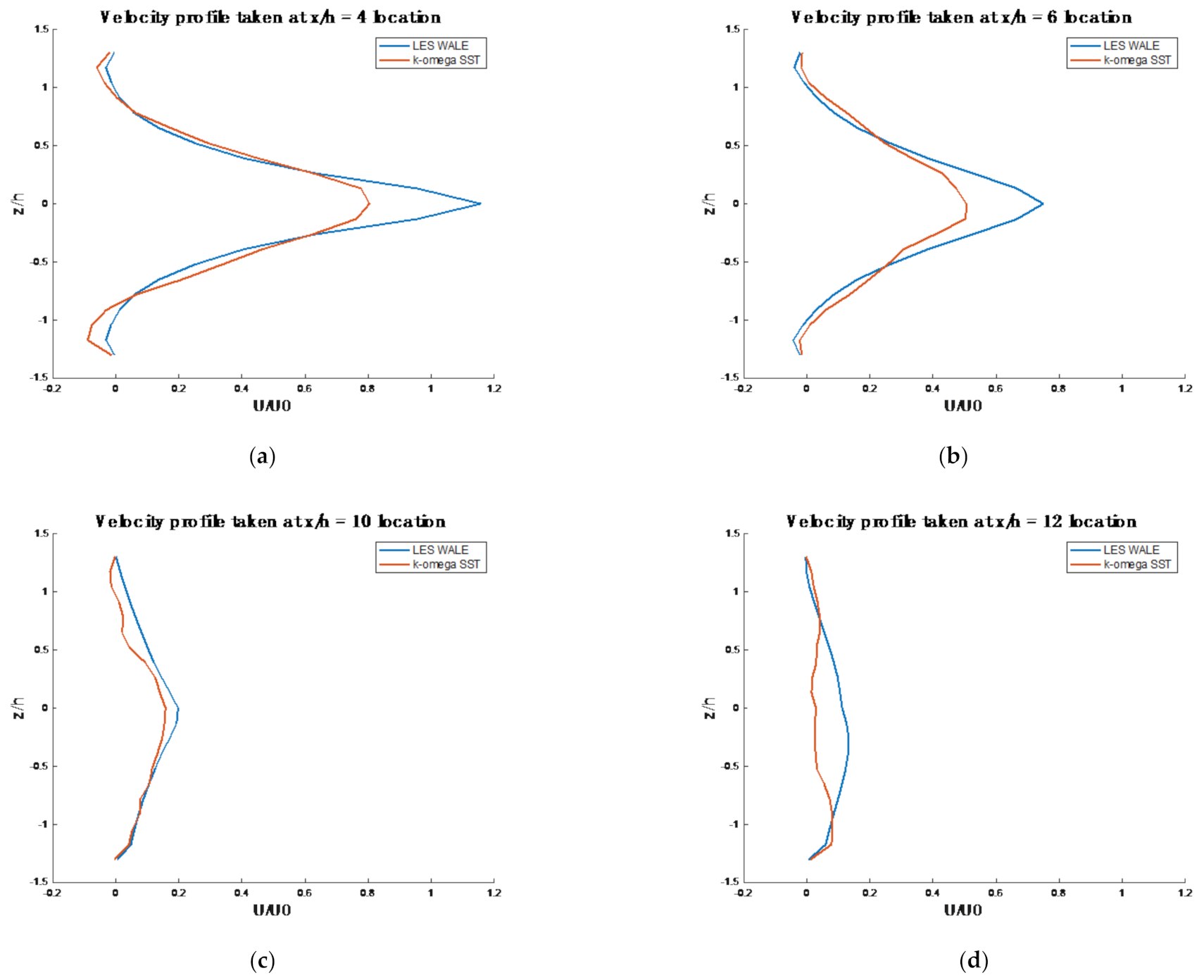
Figure 11 represents the velocity profile from the left to right plane. As Figure 10 shows, there was not much difference between the two models. and in Figure 11, this trend was maintained. Moreover, the affirmation that the reattachment point was between x/h = 6 and x/h = 10 was also maintained, because the negative speed values disappeared between these positions.

In Figure 10a and Figure 11a, divergences were found in the mean velocity profiles predicted by the two turbulence models. The reason could be found in the fact that LES-based models have a higher resolution capacity than k-omega SST. The region where the x/h = 4 profile was located was the most turbulent one. Therefore, as the used turbulence models were different, this was the area where the largest differences appeared. In LES, the filter is spatially based, and performs to decrease the amplitude of the scales of motion. Usually, LES models resolve the largest scales of turbulence, whereas in RANS, the time filter removes the scales of motion with time scales less than the filter width.

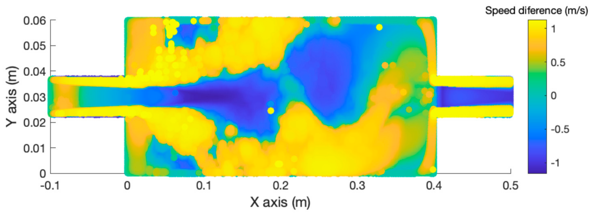
At this point in the simulation, the mean velocity of both models was compared by subtracting the average speed of the LES WALE cell from the mean velocity of the k-omega SST cell to obtain the relative variance between them, as Figure 12 illustrates.

The maximum, minimum, mean, and mode errors were 1.1335 m/s, –1.1589 m/s, –0.023 m/s, and –0.00028 m/s, respectively. Despite having a velocity variation of 2.29 m/s between the maximum and minimum error, the mode revealed that the largest frequency variation between the models was not very high. Furthermore, the mean square error value, if calculated, would be 0.008 ${\mathrm{m}}^2/{\mathrm{s}}^2$. Therefore, both models had very similar behavior.

However, in the sudden expansion from position x= 0 to x = 0.1 m, the highest variance values were found. In this zone, the turbulence models differed from each other more, and this result is also shown in Figure 10a,b and Figure 11a,b, where the U/U₀ values had more variance. In addition, after the reattachment point $X_r \approx 0.196 \mathrm{m}$ and up to the contraction zone, the differences between the two models were minimal.

Therefore, during fluid expansion or contraction, the model estimations differed from each other more because of the equations used to solve the turbulence. Nevertheless, after analyzing the mean square error and mode, the values confirmed that both had, in general, a minimum variance.

4. Discussion

The simulations concluded with two different values of reattachment length: $X_r{}_{SST}=0.196 \mathrm{m}$ and $X_r{}_{LES}=0.18 \mathrm{m}$. The expansion ratio was $E_r=\frac{60 \mathrm{mm}}{14 \mathrm{mm}}=4.28$ (see [38]). To compare with the experiment by Wang et al. [23], whose result is represented in Figure 13, the Reynolds number should have been calculated by adopting Equation (9) (see Wang et al. [23]), where $U_b$ was the speed at $1·h$ and the cinematic viscosity was $v=1.004·{10}^{-6}{\mathrm{m}}^2$/$\mathrm{s}$ at 20 °C.

$$R{e}_{h_{SST}}=\frac{U_b·h}{v}=\frac{0.256·0.023}{1.004·{10}^{-6}}=6489.81$$

(10)

$$\frac{X_{r_{SST}}}{h}=\frac{0.196}{0.023}=8.52$$

(11)

Therefore, the k-omega SST model had an $X_{r_{SST}}=8.52·h$ (see Equation (11)) for a $R{e}_h{}_{SST}=6489.81$, which was outside any other experiment (Figure 13). This phenomenon occurred due to the step ratio. In Wang et al. [23], it was smaller than that of the present study; specifically, Wang et al. [23] had $E_r=2:1,$ and this work had a ratio of $E_r=30:7$, which corresponds to a 2.14 times more expansive duct. The other reason may have been because the k-omega SST model was not the best way to estimate it. This is why the LES model was adopted: to compare both models and obtain better performance. Another issue is that the results presented in Figure 13 adopted a non-symmetric, single-step geometry, while in the present study, a 3D geometry was adopted.

It seems logical that when reviewing the LES results with Figure 13, the $R{e}_{h_{LES}}$ had to be calculated. However, the speed at point $x=1·h$ was $U_b=0.25\mathrm{m}/\mathrm{s}$, which was almost identical to the k-omega SST; hence, $R{e}_{h_{SST}}\approx R{e}_{h_{LES}}$. The reattachment length point was very close to the k-omega SST model, and the value was $X_{r_{LES}}/h=7.82$. This parameter was closer to that found in the Fan et al. [22] experiment. Therefore, it seems that the LES WALE performed better than the k-omega SST, but there was still a difference in the X_r/h values.

Using the actual results of the LES WALE and k-omega SST, the mechanical losses were calculated to compare the difference between the Borda–Carnot equations and the simulations. Thus, for position 0 and position 1 in Figure 4, the mean velocity was calculated. To obtain the mean velocity of the position 1 section, the inspection plane was fixed after the reattachment point. For position 0, the mean velocity was 1 m/s for the LES WALE and k-omega SST. However, at position 1, there were some speed differences. For the LES WALE, the average velocity was 0.048 m/s, and when adopting Equation (1), the mechanical loss was 452.2 $\mathrm{J}/{\mathrm{m}}^3$. Nevertheless, for the k-omega SST, the mean speed was 0.042 m/s, so the loss was 457.76 $\mathrm{J}/{\mathrm{m}}^3$. The theorical value was $457.04\mathrm{J}/{\mathrm{m}}^3$, which was more or less the value obtained in the simulation, although the k-omega SST differed more from the estimated value.

For the contraction mechanical loss, Equation (5) was used, which required U₁ velocity. That speed in the simulations was 0.048 m/s for the LES WALE model and 0.042 m/s for the k-omega SST. Thus, the mechanical loss for the contraction with the LES WALE was 198.7 $\mathrm{J}/{\mathrm{m}}^3$, and for k-omega SST, it was 152.13 $\mathrm{J}/{\mathrm{m}}^3$. Both values were very close to the theorical value of 171.91$\mathrm{J}/{\mathrm{m}}^3$.

5. Conclusions

This study concluded that the LES WALE had more speed variance than the RANS model. The reattachment point could be settled in the $X_r{}_{LES}\approx 0.18 \mathrm{m}$ position for the LES WALE and the $X_r{}_{SST}\approx 0.19 \mathrm{m}$ position for the k-omega SST. The reattachment length was estimated by adopting the constant $X_r=8.52·h$ for the k-omega SST and $X_r=7.82·h$ for the LES WALE, which were calculated for a specific $R{e}_h=6489.81$ with a given $E_r=30:7$. The LES WALE result was better than the k-omega SST when compared to the experiments of other authors.

In addition, the plot of the velocity variance at different x/h positions revealed that the fluid behavior for both models was practically identical, and there was a small difference in the $U/U_0$ rate values.

To obtain these results, the mesh had been checked by estimating several parameters, such as the cell skewness angle and cell quality. All of them had a good result, although the cell skewness angle in 10 cells had a higher value than 90°. Despite having bad results in these 10 cells, they were insignificant, as there were more than 11 million cells in the whole geometry.

Moreover, the LES WALE model required another evaluation technique, the Taylor length scale $\left(\lambda \right)$. This value had to be examined to verify sufficient mesh resolution, and the resolution $\left(∆=\sqrt[3]{V_{cell}}\right)$ had to be at least on the order of $\left(\lambda \right)$ to fully resolve the Taylor length scale. After performing the experiment, the mesh designed for the current work was approved for developing a LES simulation. Hence, the simulation results were considered reliable.

Note that there were some mechanicals losses because of the sudden expansion and contraction of the pipe. The sudden expansion losses were about $457.04\mathrm{J}/{\mathrm{m}}^3$, while those of the sudden contraction were $171.99\mathrm{J}/{\mathrm{m}}^3$. Both parameters were estimated by adopting Borda–Carnot equations. Furthermore, the estimated values were compared with the values of the LES WALE and k-omega SST, which were almost identical.