
A Three-Function Variational Principle for Stationary Nonbarotropic Magnetohydrodynamics


1
Department of Electrical & Electronic Engineering, Faculty of Engineering, Ariel University, Ariel 40700, Israel
2
Center for Astrophysics, Geophysics and Space Sciences (AGASS), Ariel University, Ariel 40700, Israel
3
Princeton Plasma Physics Laboratory, Princeton University, Princeton, NJ 08543, USA
Symmetry 2021, 13(9), 1632; https://0-doi-org.brum.beds.ac.uk/10.3390/sym13091632
Submission received: 8 August 2021
/
Revised: 27 August 2021
/
Accepted: 2 September 2021
/
Published: 5 September 2021
(This article belongs to the Special Issue Symmetry in Fluid Flow II)
Abstract
:The current paper is devoted to the introduction of simpler Eulerian variational principles from which all the relevant equations of nonbarotropic stationary magnetohydrodynamics can be derived for magnetic fields that lie on surfaces. A variational principle is given in terms of three independent variables for stationary nonbarotropic magnetohydrodynamic flows. This is a smaller number of variables than the eight variables that appear in the standard equations of nonbarotropic magnetohydrodynamics, which are the magnetic field, the velocity field, the specific entropy, and the density. We further investigate the case in which the flow along magnetic lines is not ideal.
1. Introduction
Variational principles for magnetohydrodynamics (MHD) were introduced previously in both Lagrangian and Eulerian approaches. Sturrock [1] studied in his book a Lagrangian variational formalism for MHD. Vladimirov and Moffatt [2] in a list of works studied a Eulerian variational approach for incompressible MHD. However, their variational approach contained three more variables in addition to the seven functions that appear in the standard equations of incompressible MHD, which are the magnetic field , velocity field , and pressure P. Kats [3] extended Moffatt’s work to compressible nonbarotropic flows, but without minimizing the number of variables and thus the computational load. Moreover, Kats demonstrated that the functions he suggested can be used to describe the motion of discontinuity surfaces [4,5]. Sakurai [6] suggested a two-function Eulerian variational principle for force-free magnetohydrodynamics and used it as a basis of a numerical scheme; his method was discussed in [1]. A method of analyzing the equations for those two variables was suggested in [7]. Yahalom and Lynden-Bell [8] combined the work of Sturrock [1] with the work of Sakurai [6] to obtain a Eulerian variational principle for barotropic MHD, which depends on only six variables. The variational derivative of the suggested action produced all the equations needed to describe barotropic MHD without additional constraints. The equations obtained were similar to the ones of Frenkel, Levich, and Stilman [9] (and also those of [10]).Yahalom [11] showed that for barotropic MHD, four functions suffice. Moreover, it was demonstrated that the discontinuities of some of those variables [12] are topological local conserved quantities.
Previous work has been concerned with barotropic MHD in which the pressure and internal energy depend only on the density and not on the specific entropy and temperature. Variational principles of nonbarotropic MHD in which the internal energy and pressure are entropy dependent and thus temperature dependent effects can be described can be found in the work of Bekenstein and Oron [13] in terms of 15 functions and A. V. Kats [3] in terms of 20 functions. We mention also the cases of incompressible flows in which density does not change in time or space and isochoric flows in which the volume of a system remains constant, which are incompressible if the specific volume in the flow is also constant; however, those cases are beyond the scope of the current work. A. V. Kats in an outstanding paper [14] (Section IV, E) demonstrated that there is a large symmetry group (which may be considered a type of gauge freedom) associated with the choice of variables, and it follows that the number of functions can be reduced.Yahalom [15,16] showed that five variables suffice to describe nonbarotropic MHD for the case in which we require a Sakurai [6] form for the magnetic field. Morrison [17] introduced a Hamiltonian formalism, but this also depends on eight canonical variables (see Table 2 in [17]).The paper of Yahalom [15] was concerned with general MHD nonstationary flows. A subsequent paper [18] was concerned with stationary flows and introduced and eight-variable stationary variational principle; here, we shall attempt to improve on this and obtain a three-variable stationary variational principle for nonbarotropic MHD. This will be done for a general case in which the magnetic field lines need not lie on entropy surfaces; for the restricted case in which the magnetic field lines lie on entropy surfaces, see [19].
Applications of this paper may arise for both linear and nonlinear stability analysis of stationary nonbarotropic MHD flows [20,21] and for designing numerical algorithms for integrating the equations of MHD [22,23,24]. Another possible application is connected to obtaining new analytic solutions in terms of the variational functions [25], as will be described below.
The plan of this work is as follows: We introduce the standard notations and equations of nonbarotropic magnetohydrodynamics for the stationary and nonstationary cases. Then, we introduce the notions of load and metage. The variational principles follow.
2. Standard Formulation of Nonbarotropic Magnetohydrodynamics
The standard set of equations solved for nonbarotropic magnetohydrodynamics are given below:
Here is the partial temporal derivative, is the material derivative, and is the standard nabla operator of vector calculus. is the magnetic field. is the velocity field. is the fluid mass density. s is the specific entropy (entropy per unit mass). Finally, is the pressure, which depends on both the density and entropy (and not just the density) through the thermodynamic equation of state (the nonbarotropic case).
The justification for these equations can be found in standard books on MHD [1]. The above is valid for a collision-dominated plasma in local thermodynamic equilibrium. Such conditions are not always fulfilled by real physical plasmas, certainly not in astrophysics or in fusion-relevant magnetic confinement studies. Yet, it is thought that the fastest macroscopic instabilities obey the above equations [12], while instabilities associated with viscous or finite conductivity terms take longer. According to a theorem by Bateman [26], every system can be described by a variational principle (including viscous plasma); the challenge is to discover a compact action functional that depends on a small amount of variational functions. This paper discusses only ideal MHD, while viscous MHD will be left for future endeavors.
Equation (1) describes magnetic field lines that are moving with the fluid (“frozen” lines). Equation (2) dictates a solenoidal field. Equation (3) dictates mass conservation. Equation (4) is the Euler equation for which pressure and the Lorentz forces apply. The term:
is the electric current density. Equation (5) is due to the lack of heat generation (null viscosity and null resistivity) in ideal nonbarotropic MHD and a lack of heat conduction; thus, the only remaining thermal process is heat convection. One needs to solve for eight variables () eight equations (Equations (1) and (3)–(5)). Equation (2) is an initial condition on the field and is satisfied automatically later due to Equation (1). For the stationary case, we obtain:
3. Variational Principle of Nonbarotropic MHD
Here, we generalize the analysis of [8] for the nonbarotropic case. Let the action be:
is the internal energy per mass. We recall the thermodynamic identities:
In the above, T is the temperature and w is the specific enthalpy. is the specific internal energy. T is the temperature. w is the specific enthalpy. A special case of the equation of state is the polytropic equation of state [27]:
K and may depend on the specific entropy s. Hence:
the last identity is up to a function dependent on s. Obviously, are Lagrange multipliers, which are inserted in such a way that the variational principle yields the following equations:
may be multiple-valued. If does not vanish, these are just the continuity Equation (3), entropy conservation, and a declaration that Sakurai’s functions are moving with the flow. Varying with respect to , we obtain:
Hence, is given in Sakurai’s form and thus respects Equation (2). It can be shown that if is in Sakurai’s form and Equation (16) is fulfilled, then it follows that also Equation (1) is respected.
We showed that the entire set of equations of nonbarotropic MHD is obtained from the above action except Euler’s equations. We now take care of that. Let us vary the above action with respect to :
is zero in generic cases. For astrophysical scenarios, on the boundary of the flow domain; in the case of a fluid contained in some pipe, the conditions are imposed ( denotes the unit vector normal to the boundary). on the cut of is zero if is single-valued and , which is the case for generic topologies. For , which is multiple-valued, only a Kutta velocity variation [28] that is parallel to the cut will remove the cut integral. An arbitrary velocity variation on the cut dictates on said surface, which contradicts the notion that a cut is arbitrary, as is the zero line of the azimuth. Later, we demonstrate that the “cut” is comoving; thus, it may become quite involved. This difficult reality may be more convenient to handle in symmetrical cases.
If the surface integrals vanish and also we have for an arbitrary velocity variation, we find that:
This resembles the Clebsch form in nonmagnetic fluids [29,30]. Taking the variation with respect to , we have:
is the enthalpy per mass. Provided vanishes on the boundary and vanishes on the cut of for , which is multiple-valued (thus, either a Kutta-type condition for the velocity in contradiction with the “cut” being an arbitrary surface or a vanishing density variation on the same) and in the beginning and the end, the following equation results:
Since the right-hand side of the equation is single-valued as it is composed of physical variables that are not potentials, we obtain:
Thus, the cut is comoving with the flow and may become complicated. This situation may be less restrictive when the flow is symmetrical.
Finally, we vary with respect to both and , leading to the following expressions:
If the temporal and boundary conditions are satisfied with respect to the variations and on the domain boundary and on the cuts for the case that some (or all) of the relevant variables are multiple-valued, we obtain the following equations:
in which Equation (3) is used. By suitable temporal conditions, we require that and vanish at the initial and final times. Cases making the boundary term null include a boundary located at infinity in which both and are null or a boundary that is impermeable and perfectly conducting. For the integral over the “cuts” to become null, one can use and , which are single-valued. It is shown that can always be single-valued; hence, taking to be single-valued is not a restriction. In some topologies, is multiple-valued, and for those cases, a single-valued suffices to make the cut term vanish.
Finally, we take a variation of the action with respect to s:
in which the temperature is . We notice that according to Equation (19), is single-valued, and hence, no cuts are needed. Taking into account the continuity Equation (3) we obtain for locations in which the density is not null, the result:
provided that vanishes for an arbitrary .
4. Euler’s Equations
We shall now show that a velocity field given by Equation (19), such that the equations for satisfy the corresponding Equations (16), (21), (25), and (27) must satisfy Euler’s equations. Let us calculate the material derivative of :
It can be easily shown that:
is a Cartesian coordinate, and a summation convention is assumed. Inserting the result from Equations (16) and (29) into Equation (28) yields:
Equations (17) and (19) are used. This shows that the nonbarotropic MHD Euler equations can be obtained from the action of Equation (12), and thus, all the equations of nonbarotropic MHD can be derived from the action for arbitrary volume variations restricted only on the relevant boundaries and cuts. Boundary variations serve to obtain boundary and initial conditions for the equations.
5. Simplified Action
It might be argued that the above claims are misleading. A simplified action for nonbarotropic MHD is presented, and instead, six more functions are added to . The action described in Equation (12) in a pedagogical form can be simplified. It is clear that the Lagrangian density of Equation (12) can be written as:
is a shorthand notation for (see Equation (19)), and is a shorthand notation for (see Equation (17)). Thus, has four contributions:
The only term containing is ( depends on , but being a boundary term in space and time, it does not affect the derived volume equations) . After we equate to zero the variational derivative with respect to , we obtain Equation (19), but this will otherwise have no effect on the other variational derivatives. The only term depending on is , and this term will lead, after we set the variational derivative to zero, to Equation (17), but will not change other variations. contains only complete partial derivatives and thus does not contribute to the equations, although it can influence the boundary conditions. Thus, Equations (16), (21), (25) and (27) are derived from:
in which replaces and replaces . After integrating Equations (16), (21), (25), and (27), we are allowed to insert the potentials into Equations (17) and (19), thus deriving the vector fields and . To summarize, we showed that the general ideal nonbarotropic MHD problem is reduced from eight equations (Equations (1) and (3)–(5)) and the additional constraint (Equation (2)) to a problem of eight first-order (in the temporal derivative) unconstrained equations. This set of equations can be derived from the Lagrangian density .
6. Stationary Nonbarotropic MHD
Stationary configurations are unique to Eulerian fluid dynamics with no counterpart in the Lagrangian description of fluid dynamics. Stationary configurations are defined by the fact that the fields are independent of time. This does not imply that the potentials are functions of only the spatial coordinates. Indeed, choosing the potentials in such a way will lead to erroneous results such that the stationary equations of motion can not be derived from of Equation (32). This problem can be solved as follows. Let us choose to depend on the spatial coordinates alone. is chosen such that:
in which depends on the spatial coordinates alone. of Equation (32) will become:
This can be compared with [2] (Equation 6.12) for incompressible flows in which their I is analogous to our . Notice that is not a conserved quantity, but I is conserved.
Varying the Lagrangian with respect to leads to the following equations:
These lead to the stationary nonbarotropic MHD equations:
In what follows, we attempt to reduce the number of variational variables from eight to three.
7. Load and Metage
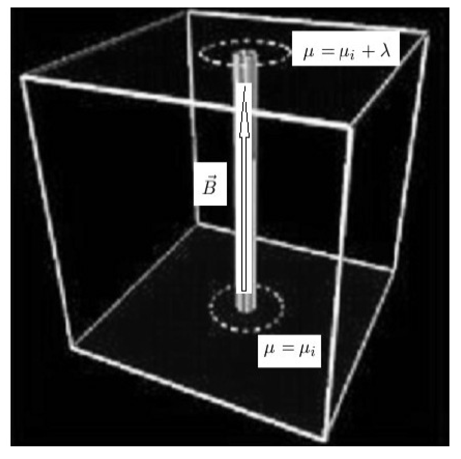
The following section follows closely a similar section in [8]. Consider a thin tube surrounding a magnetic field line as described in Figure 1. The magnetic flux contained within the tube is:
and the mass contained within the tube is:
in which is a short distance along the tube. Since the magnetic field lines are comoving as dictated by Equations (1) and (3), both the quantities and will not change during the motion of the tube. Since the tube is thin, we may define the comoving magnetic load:
calculated along the field line. The parts of the magnetic line that go out of the flow region to parts of space in which have zero contribution. is single-valued, which can be experimentally measured in principle. Since is comoving, it satisfies:
Furthermore, surfaces of constant magnetic load are comoving and are made from magnetic field lines. Hence, the gradient to such surfaces must be normal to the surface, hence orthogonal to the field lines:
Consider an arbitrary comoving point on the field line denoted by i, and consider another comoving point on the field line and mark it as r. The integral:
is also a comoving quantity, which we denote after Lynden-Bell and Katz [31] as the magnetic metage. is a number that can be chosen differently for each line. Thus:
By differentiating along the field line, we derive:
will be generally multiple-valued.
We now have two comoving coordinates of flow, ; obviously, in a three-dimensional flow, we should also have a third. However, before defining the third function, we first change to a specific function of . Consider the magnetic flux within a load surface . The magnetic flux is a comoving quantity and depends only on of its boundary. Define:
satisfies the equations:
Let us define . Since is not orthogonal to , we can choose to be orthogonal to and not be in the direction of . We chose not to depend uniquely on . Both and are orthogonal to , so it must be that:
However, using Equation (2), we have:
This implies that A is a function of . Now, we can define a new comoving function such that:
In terms of this function, we obtain the Sakurai (Euler potentials) presentation:
We thus showed how can be practically defined for a given . is defined in a nonunique way since one can redefine by performing: in which is any arbitrary function. serve as labels of the field lines. Moreover, we obtain the following expression for the magnetic flux:
In the case that the surface integral is performed inside a load contour, we obtain:
In one case, the load surfaces are topological cylinders. is thus multiple-valued, and we obtain the upper value. In the second case, the surfaces of constant load are topological spheres, and is single-valued and has both minimal and maximal values. Hence the lower value of is obtained. In some cases, is identical to twice the latitude angle . In those cases, (value at the “north pole”) and (value at the “south pole”).
Comparing with Equation (47), it follows that can be either single-valued or multiple-valued and that its discontinuity across its cut in the multiple-valued scenario is .
So far, the discussion has not differentiated the cases of stationary and nonstationary flows. It should be noted that even for stationary flows, one can have a nonstationary coordinate as the magnetic field depends only on the gradient of (see Equation (52)), in particular if is stationary, then , which is clearly not stationary, will produce according to Equation (52) a stationary magnetic field. In what follows, it is advantageous to use the form of given in Equation (34) in which is stationary.
are sufficient to label any fluid element in three dimensions. However, for a nonbarotropic ideal flow, there is also another possible label, s, which is comoving due to Equation (5). The question then arises about the relation of s to the other labels. Since we need to decide regarding the preferred set of labels, it may seem that the physical labels are , which are the surfaces on which the magnetic fields lie and the entropy. Thus, is a function of . If the magnetic field lines lie on the entropy surface, is an independent label. The density is:
can be defined for each line separately according to Equation (44), and it is thus obvious that such a choice exists in which is uniquely a function of s. One may also think of the entropy s as functions . In what follows, we shall ignore the status of s as a label and consider it as a variational function, which only attains the status of a label at the variational extremum.
8. A Simpler Variational Principle of Stationary Nonbarotropic Magnetohydrodynamics
In a previous paper [18], we showed that stationary nonbarotropic magnetohydrodynamics can be described in terms of eight first-order differential equations and by an action principle from which those equations can be derived. Below, we show that one can do better for the case in which the magnetic field lines lie on an entropy surface; in this case three functions suffice to describe stationary nonbarotropic magnetohydrodynamics.
Consider Equation (48); for a stationary flow, it takes the form:
Hence, can take the form:
However, the velocity field must satisfy the stationary mass conservation Equation (3):
A sufficient condition (although not necessary) for to be a solution of Equation (58) is that is of the form ; here, N is arbitrary. Thus, can be written as:
Let us now calculate in which is given by Sakurai’s presentation Equation (52):
N can be at most a function of the three coordinates ; hence:
Rearranging terms and using Equation (52), we can write:
However, using Equation (46), this simplifies to the form:
However, since N is at most a function of , it follows that is some function of :
This can be easily integrated to yield:
We shall replace with defined as:
This does not affect Equation (52) as:
However, the velocity takes a simpler form:
. We recall that is defined in Equation (44) up to a constant, which may vary between field lines. As the lines are labeled by their values, we can add a function of to without affecting its desired properties. We thus define in the form:
can be nonsingle-valued. Inserting Equation (72) into Equation (71) leads to:
The primes on will be ignored from now on. This is analogous to [2] (Equation 7.11) for incompressible flows; our and resemble their A and . satisfies the following:
where we used Equation (45) and (52). are both comoving and stationary. satisfies Equation (34). If:
is a local vector basis at any point in space, then their exists a dual basis:
such that:
is Kronecker’s delta. The surfaces generate a local vector basis for space, while the physical fields of interest are contained in the dual basis. We can now construct a vector product of and , and taking into account Equations (52) and (73), we arrive at the equation:
thus, and lie on surfaces and are a vector basis for this two-dimensional surface. This can be compared with [2] (Equation 5.6) for incompressible flows; the J appearing in that paper is analogous to .
9. A Three-Function Variational Principle for Stationary MHD
Previously, we demonstrated that, provided that the is given by Equation (73) and is given by Equation (52), then Equations (7)–(9) are satisfied. To complete the set of equations we show how the Euler Equation (4) can be derived from the action:
in which both and are given by Equations (52) and (73), respectively, and the density is given by Equation (45):
The Lagrangian density of Equation (79) takes the more explicit form:
and can be seen explicitly to depend on only three functions. We underline that the magnetic field lines lie on entropy surfaces. s must be a function of only and does not depend on . Let us make arbitrary small variations of the functions . Let us define a variation that does not modify the ’s, such that:
in which is the Lagrangian displacement; thus:
This leads to the equation:
Making a variation of given in Equation (80) with respect to yields:
Making a variation of s results in:
Furthermore, taking the variation of given by Sakurai’s Equation (52) with respect to yields:
It remains to calculate by varying Equation (73); this yields:
Varying the action results in:
Using the well-known vector identity:
and the theorem of Gauss, we can write now Equation (89) in the form:
Time integration is of no consequence in the above. Notice that we used Equation (6) and the vorticity . If for , nullifying the boundary term, but otherwise arbitrary, then:
Using the well-known vector identity:
and rearranging terms, we recover the stationary Euler equation:
10. An Application: Helical Stratified Magnetic Field
10.1. The Magnetic Field and Related Labels
Consider [32] a magnetohydrodynamic flow of uniform density . Furthermore, assume that the flow contains a helical stratified magnetic field:
are cylindrical coordinates. are unit vectors. are constants. The field is confined to a cylinder of radius a and does not depend on z. We assume that and are identified such that a topological torus is realized. The only field lines that will be closed are such that:
Lines not satisfying this condition are surface-filling. The field lines lie on cylindrical surfaces, so one can calculate the flux through a circular surface lying on the plane z and bounded by R. The flux is:
The function can now be calculated according to Equation (47) to yield the value:
Solving Equation (17) for , we obtain the following nonunique solution:
Finally, we solve Equation (46) for ; here, we suggest the following simple and nonunique solution:
Thus, surfaces are just z planes. Notice that since we have identified the planes and , is nonsingle-valued. The same can be said to be on , which is doubly nonsingle-valued in both the z and directions.
10.2. The Velocity Field
11. The Three-Function Action Principle for a Static Configuration
The static configuration is a stationary flow such that . In this case, the mass conservation Equation (7) and magnetic field Equation (9) are satisfied trivially. To complete the set of equations, we show how the static Euler Equation (4) can be derived from the action:
in which is given by Equation (52) and the density is given by Equation (80). The Lagrangian density of Equation (105) can be put in the more explicit form:
Varying the action results in:
Using the well-known vector identity (Equations (91)) and the theorem of Gauss, we can write now Equation (107) in the form:
The time integration is of no consequence in the above expression. We used Equation (6). If for an arbitrary , but such that the boundary term is null, then we obtain:
and rearranging terms, we recover the stationary Euler equation:
12. Transport Phenomena
In many plasmas including static configurations, heat is transferred preferably along magnetic field lines:
in which is a tensor of heat conductivity. This tensor is usually larger in the magnetic field direction and thus can be written as:
In the above, is a unit vector in the magnetic field direction, ⊗ is the tensor product, I is the unit matrix, is the heat conductivity in the directions perpendicular to the magnetic field lines, and is the larger heat conductivity in the direction parallel to the magnetic field lines. The equation for a stationary heat flux configuration is:
This equation can be derived from the heat Lagrangian and Lagrangian density:
In the above, is the transpose of , , and the Einstein summation convention is assumed. Taking the variation with respect to the temperature T yields:
hence:
and using the theorem of Gauss:
thus for appropriate boundary conditions, we derive Equation (114). We notice that heat conduction is not taken into account in ideal MHD, which only assumes the convection of heat. However, provided that conduction is seen as a secondary process with respect to convection, we may obtain using the ideal variational principle a stationary or static magnetic field configuration using the appropriate variational expression given in previous sections. Then using the known magnetic field configuration, we derive the appropriate heat flux transport using .
13. Conclusions
It is shown that stationary nonbarotropic magnetohydrodynamics can be derived from a variational principle of three functions. We showed this for both the stationary and static cases.
Possible applications include stability studies of stationary MHD and the development of numerical methods for integrating MHD equations. It may be possible to incorporate the current formalism in existing codes instead of developing a new code from scratch. Possible codes were described in [33,34,35,36,37]. We anticipate applications of this work to linear and nonlinear stability studies of known MHD configurations [20,21,38]. To achieve this, we may need to add additional constants of motion constraints to the action [39,40,41,42,43]. As for designing numerical methods for integratingthe equations of MHD, one may follow the approach described in [22,23,24,28].
Another application of the variational variables is obtaining analytic solutions for the MHD equations. Although the equations are very difficult to solve, both being partial differential equations and nonlinear, possible solutions can be found using variational functions. An example for this approach is the self-gravitating torus described in [25] and also in Section 10.
One can use continuous symmetries that appear in the action to derive through the Noether theorem new conservation laws. An example of such a derivation can be found in [32,44].
Topological invariants have always been useful, and there are such invariants in MHD flows. For example, the two helicities (magnetic helicity and cross-helicity) have long been useful in research into the problem of hydrogen fusion and in various astrophysical scenarios. In previous studied [8,12,45], relations between the helicities and symmetries of MHD were made. Furthermore, the functions of the current action are helpful for identifying and characterizing new topological invariants in MHD [32,46,47].
Although ideal MHD does not describe real plasmas fully, we showed here how processes such as heat conduction can be also described using variational analysis provided that the magnetic field configuration is given approximately by ideal variational analysis.
To conclude, we underline the limitations of the current work. First, MHD is a fluid theory and as such misses some of the processes that can only be addressed by a detailed kinetic model. Second, ideal MHD considered here neglects important nonideal processes such as resistive heating, heat conduction, and viscous effects. Moreover, we assume magnetic fields that lie on surfaces (that is Equation (17)), while for some MHD configurations, magnetic field lines are volume filling; for such cases, the current approach is not applicable.
Funding
This research received no external funding.
Institutional Review Board Statement
Not applicable.
Informed Consent Statement
Not applicable.
Data Availability Statement
Not applicable.
Acknowledgments
The author wishes to thank Allan Reiman of Princeton University for discussions and helpful comments and for suggesting some of the sections in the current paper.
Conflicts of Interest
The author declares no conflict of interest.
References
- Sturrock, P.A. Plasma Physics; Cambridge University Press: Cambridge, MA, USA, 1994. [Google Scholar]
- Vladimirov, V.A.; Moffatt, H.K. On general transformations and variational principles for the magnetohydrodynamics of ideal fluids. Part 1. Fundamental principles. J. Fluid. Mech. 1995, 283, 125–139. [Google Scholar] [CrossRef]
- Kats, A.V. Los Alamos Archives physics-0212023 (2002). JETP Lett. 2003, 77, 657. [Google Scholar] [CrossRef]
- Kats, A.V.; Kontorovich, V.M. Hamiltonian description of the motion of discontinuity surfaces. Low Temp. Phys. 1997, 23, 89. [Google Scholar] [CrossRef]
- Kats, A.V. Variational principle and canonical variables in hydrodynamics with discontinuities. Phys. D Nonlinear Phenom. 2001, 459, 152–153. [Google Scholar] [CrossRef]
- Sakurai, T. A New Approach to the Force-Free Field and Its Application to the Magnetic Field of Solar Active Regions. Publ. Astron. Soc. Jpn. 1979, 31, 209–230. [Google Scholar]
- Yang, W.H.; Sturrock, P.A.; Antiochos, S. Force-free magnetic fields—The magneto-frictional method. Astrophys. J. 1986, 309, 383–391. [Google Scholar] [CrossRef]
- Yahalom, A.; Lynden-Bell, D. Simplified Variational Principles for Barotropic Magnetohydrodynamics. J. Fluid. Mech. 2008, 607, 235–265. [Google Scholar] [CrossRef] [Green Version]
- Frenkel, A.; Levich, E.; Stilman, L. Hamiltonian description of ideal MHD revealing new invariants of motion. Phys. Lett. A 1982, 88, 461–465. [Google Scholar] [CrossRef]
- Zakharov, V.E.; Kuznetsov, E.A. Hamiltonian formalism for nonlinear waves. Phys.-Uspekhi 1997, 40, 1087. [Google Scholar] [CrossRef]
- Yahalom, A. A Four Function Variational Principle for Barotropic Magnetohydrodynamics. EPL Europhys. Lett. 2010, 89, 34005. [Google Scholar] [CrossRef]
- Yahalom, A. Aharonov–Bohm Effects in Magnetohydrodynamics. Phys. Lett. A 2013, 377, 1898–1904. [Google Scholar] [CrossRef]
- Bekenstein, J.D.; Oron, A. Conservation of circulation in magnetohydrodynamics. Phys. Rev. E 2000, 62, 5594–5602. [Google Scholar] [CrossRef] [Green Version]
- Kats, A.V. Canonical description of ideal magnetohydrodynamic flows and integrals of motion. Phys. Rev E 2004, 69, 046303. [Google Scholar] [CrossRef] [Green Version]
- Yahalom, A. Simplified variational principles for nonbarotropic magnetohydrodynamics. J. Plasma Phys. 2016, 82, 905820204. [Google Scholar] [CrossRef] [Green Version]
- Yahalom, A. Non-Barotropic Magnetohydrodynamics as a Five Function Field Theory. Int. J. Geom. Methods Mod. Phys. 2016, 13, 1650130. [Google Scholar] [CrossRef]
- Morrison, P.J. Poisson Brackets for Fluids and Plasmas. AIP Conf. Proc. 1982, 88, 13–46. [Google Scholar]
- Yahalom, A. Simplified Variational Principles for Stationary non-Barotropic Magnetohydrodynamics. Int. J. Mech. 2016, 10, 336–341. [Google Scholar]
- Yahalom, A. A Simpler Variational Principle for Stationary non-Barotropic Ideal Magnetohydrodynamics. Chaotic Model. Simul. 2018, 1, 19–33. [Google Scholar]
- Vladimirov, V.A.; Moffatt, H.K.; Ilin, K.I. On general transformations and variational principles for the magnetohydrodynamics of ideal fluids. Part 4. Generalized isovorticity principle for three-dimensional flows. J. Fluid Mech. 1999, 390, 127–150. [Google Scholar] [CrossRef]
- Almaguer, J.A.; Hameiri, E.; Herrera, J.; Holm, D.D. Lyapunov stability analysis of magnetohydrodynamic plasma equilibria with axisymmetric toroidal flow. Phys. Fluids 1988, 31, 1930–1939. [Google Scholar] [CrossRef]
- Yahalom, A. Method and System for Numerical Simulation of Fluid Flow. U.S. Patent 6,516,292, 4 February 2003. [Google Scholar]
- Yahalom, A.; Pinhasi, G. Simulating Fluid Dynamics Using a Variational Principle. In Proceedings of the 41st Aerospace Sciences Meeting and Exhibit (AIAA), Reno, NV, USA, 6–9 January 2003. [Google Scholar]
- Ophir, D.; Yahalom, A.; Pinhasi, G.; Kopylenko, M. A Combined Variational and Multi-Grid Approach for Fluid Dynamics Simulation. In Proceedings of the 44th AIAA Aerospace Sciences Meeting and Exhibit, Reno, NV, USA, 9–12 January 2006. [Google Scholar]
- Yahalom, A. Using fluid variational variables to obtain new analytic solutions of self-gravitating flows with nonzero helicity. Procedia IUTAM 2013, 7, 223–232. [Google Scholar] [CrossRef] [Green Version]
- Bateman, H. On Dissipative Systems and Related Variational Principles. Phys. Rev. 1931, 38, 815–819. [Google Scholar] [CrossRef]
- Binney, J.; Tremaine, S. Galactic Dynamics; Princeton University Press: Princeton, NJ, USA, 1987. [Google Scholar]
- Yahalom, A.; Pinhasi, G.; Kopylenko, M. A Numerical Model Based on Variational Principle for Airfoil and Wing Aerodynamics. In Proceedings of the 43rd AIAA Aerospace Sciences Meeting and Exhibit, Reno, NV, USA, 10–13 January 2005. [Google Scholar]
- Clebsch, A. Uber eine allgemeine Transformation der hydrodynamischen Gleichungen. J. Reine Angew. Math. 1857, 54, 293–312. [Google Scholar]
- Clebsch, A. Uber die Integration der hydrodynamischen Gleichungen. J. Reine Angew. Math. 1859, 56, 1–10. [Google Scholar]
- Lynden-Bell, D.; Katz, J. Isocirculational flows and their Lagrangian and energy principles. Proc. R. Soc. Lond. Ser. A Math. Phys. Sci. 1981, 378, 179–205. [Google Scholar]
- Yahalom, A.; Qin, H. Noether Currents for Eulerian Variational Principles in Non-Barotropic Magnetohydrodynamics and Topological Conservations Laws. J. Fluid Mech. 2021, 908, A4. [Google Scholar] [CrossRef]
- Mignone, A.; Rossi, P.; Bodo, G.; Ferrari, A.; Massaglia, S. High-resolution 3D relativistic MHD simulations of jets. Mon. Not. R. Astron. Soc. 2010, 402, 7–12. [Google Scholar] [CrossRef]
- Miyoshi, T.; Kusano, K. A multi-state HLL approximate Riemann solver for ideal magnetohydrodynamics. J. Comput. Phys. 2005, 208, 315–344. [Google Scholar] [CrossRef]
- Igumenshchev, I.V.; Narayan, R.; Abramowicz, M.A. Three-dimensional Magnetohydrodynamic Simulations of Radiatively Inefficient Accretion Flows. Astrophys. J. 2003, 592, 1042–1059. [Google Scholar] [CrossRef]
- Faber, J.; Baumgarte, T.; Shapiro, S.L.; Taniguchi, K. General Relativistic Binary Merger Simulations and Short Gamma-Ray Bursts. Astrophys. J. 2006, 641, L93–L96. [Google Scholar] [CrossRef] [Green Version]
- Hoyos, J.; Reisenegger, A.; Valdivia, J.A. Multi-Fluid Simulation of the Magnetic Field Evolution in Neutron Stars. AIP Conf. Proc. 2008, 983, 404–408. [Google Scholar]
- Bernstein, I.B.; Frieman, E.A.; Kruskal, M.D.; Kulsrud, R.M. An energy principle for hydromagnetic stability problems. Proc. R. Soc. London. Ser. A Math. Phys. Sci. 1958, 244, 17–40. [Google Scholar]
- Arnold, V.I. A variational principle for three-dimensional steady flows of an ideal fluid. Appl. Math. Mech. 1965, 29, 154–163. [Google Scholar]
- Arnold, V.I. Conditions for nonlinear stability of stationary plane curvilinear flows of an ideal fluid. Dokl. Acad. Nauk SSSR 1965, 162, 975. [Google Scholar]
- Katz, J.; Inagaki, S.; Yahalom, A. Energy Principles for Self-Gravitating Barotropic Flows: I. General Theory. Publ. Astron. Soc. Jpn. 1993, 45, 421–430. [Google Scholar]
- Yahalom, A.; Katz, J.; Inagaki, K. Energy principles for self-gravitating barotropic flows—II. The stability of Maclaurin discs. Mon. Not. R. Astron. Soc. 1994, 268, 506–516. [Google Scholar] [CrossRef] [Green Version]
- Yahalom, A. Stability in the weak variational principle of barotropic flows and implications for self-gravitating discs. Mon. Not. R. Astron. Soc. 2011, 418, 40–426. [Google Scholar] [CrossRef] [Green Version]
- Yahalom, A. A New Diffeomorphism Symmetry Group of Magnetohydrodynamics. In Lie Theory and Its Applications in Physics; Dobrev, V., Ed.; Springer: Tokyo, Japan, 2013; Volume 36, pp. 461–468. [Google Scholar]
- Yahalom, A. Helicity conservation via the Noether theorem. J. Math. Phys. 1995, 36, 1324–1327. [Google Scholar] [CrossRef] [Green Version]
- Yahalom, A. A Conserved Local Cross Helicity for Non-Barotropic MHD. J. Geophys. Astrophys. Fluid Dyn. 2017, 111, 131–137. [Google Scholar] [CrossRef] [Green Version]
- Yahalom, A. Non-Barotropic Cross-helicity Conservation Applications in Magnetohydrodynamics and the Aharanov–Bohm effect. Fluid Dyn. Res. 2017, 50, 011406. [Google Scholar] [CrossRef] [Green Version]
Figure 1.
A thin tube surrounding a magnetic field line.

Publisher’s Note: MDPI stays neutral with regard to jurisdictional claims in published maps and institutional affiliations. |
© 2021 by the author. Licensee MDPI, Basel, Switzerland. This article is an open access article distributed under the terms and conditions of the Creative Commons Attribution (CC BY) license (https://creativecommons.org/licenses/by/4.0/).
Share and Cite
MDPI and ACS Style
Yahalom, A. A Three-Function Variational Principle for Stationary Nonbarotropic Magnetohydrodynamics. Symmetry 2021, 13, 1632. https://0-doi-org.brum.beds.ac.uk/10.3390/sym13091632
AMA Style
Yahalom A. A Three-Function Variational Principle for Stationary Nonbarotropic Magnetohydrodynamics. Symmetry. 2021; 13(9):1632. https://0-doi-org.brum.beds.ac.uk/10.3390/sym13091632
Chicago/Turabian StyleYahalom, Asher. 2021. "A Three-Function Variational Principle for Stationary Nonbarotropic Magnetohydrodynamics" Symmetry 13, no. 9: 1632. https://0-doi-org.brum.beds.ac.uk/10.3390/sym13091632
Note that from the first issue of 2016, this journal uses article numbers instead of page numbers. See further details here.