
Adaptive Fuzzy Fault-Tolerant Control against Time-Varying Faults via a New Sliding Mode Observer Method


1
School of Science, Shenyang University of Technology, Shenyang 110870, China
2
College of Automation, Harbin Engineering University, Harbin 150001, China
*
Author to whom correspondence should be addressed.
†
These authors contributed equally to this work.
Symmetry 2021, 13(9), 1615; https://0-doi-org.brum.beds.ac.uk/10.3390/sym13091615
Submission received: 2 August 2021
/
Revised: 27 August 2021
/
Accepted: 29 August 2021
/
Published: 2 September 2021
(This article belongs to the Special Issue Recent Advances in Sliding Mode Control/Observer and Its Applications)
Abstract
:In this study, the problem of observer-based adaptive sliding mode control is discussed for nonlinear systems with sensor and actuator faults. The time-varying actuator degradation factor and external disturbance are considered in the system simultaneously. In this study, the original system is described as a new normal system by combining the state vector, sensor faults, and external disturbance into a new state vector. For the augmented system, a new sliding mode observer is designed, where a discontinuous term is introduced such that the effects of sensor and actuator faults and external disturbance will be eliminated. In addition, based on a tricky design of the observer, the time-varying actuator degradation factor term is developed in the error system. On the basis of the state estimation, an integral-type adaptive fuzzy sliding mode controller is constructed to ensure the stability of the closed-loop system. Finally, the effectiveness of the proposed control methods can be illustrated with a numerical example.
1. Introduction
In industrial processes, actuator and/or sensor always occur with various components faults due to unexpected physical constraints and reasons [1,2,3,4]. In order to maintain the reliability of the overall control systems, fault detection and isolation (FDI) and fault-tolerant control (FTC) have received increasing research attention during the past decade [5,6,7,8]. The design scheme of FDI is to generate a residual signal to judge whether the faults occur and provide a solution to determine the location of the faults [9,10,11]. However, in practice, it is difficult to obtain the exact information of the fault. In this sense, the fault estimate has been developed and has become an ideal design basis of FTC [12,13]. In recent years, a great number of fault estimation methods have been reported in the existing literature, for instance, nonlinear observer method, adaptive learning observer method, filter-based estimation method and differential geometry methods, etc. [14,15,16].
Consequent to the in-depth study of SMO by researchers, combined with fuzzy and adaptive technologies [17,18,19], sliding mode observers have been widely used in motors, aerial vehicle, and other fields [20,21,22,23,24]. Among these existing fault estimation approaches, sliding mode observer (SMO) [25,26,27] refers to one of the most popular nonlinear observer methods, where the fault is reconstructed by the so-called equivalent output error injection principle [14]. In this research forefront, a few fault estimation SMO results have been developed for various systems by the researchers [11,28]. In [29], a fault estimation SMO was developed for mismatched nonlinear systems with unknown disturbances, where an adaptive law was designed to update the sliding mode gain online. In [30], the authors proposed a cascaded SMO method to cope with the fault estimation problem for the case in which the first Markov matrix of the system is not a full rank. In [31,32], based on a descriptor system augmentation strategy, the authors proposed a new type of extended SMO approach, which was applied to Ito stochastic systems and Markovian jump systems, respectively.
Sliding mode control is a very effective control method, and some new ideas have been put forward recently by researchers [33,34]. Hou et al. [35] solved the chattering problem common in the sliding mode control for the servo motor system by designing a new continuous terminal sliding mode control algorithm. In [36], an optimization problem based on non-negative constraints was defined for time-varying delay systems, to obtain sliding mode surface parameters and simplify the stability analysis process. In [37], the nonlinear function with sliding variable was introduced by the approach law, which alleviates the chattering phenomenon and improves the tracking performance.
However, it should be pointed out that most existing fault estimation results are concerned only about actuator faults or sensor faults. Moreover, most of the reported work has been focused on only additive actuator fault, while multiplicative type actuator fault (also called fault degradation factor) has received little research attention. In fact, in many practical control systems such as satellite systems, the multiplicative actuator faults may always occur with a time-varying characterization. However, the existing SMO methods in the aforementioned literature cannot be applied directly to solve this design problem due to technical constraints, and only additive actuator faults are therefore considered. It is thus desirable to develop a new effective SMO approach to investigate this problem.
In this paper, we aimed to research the fault estimation and FTC design problem for the continuous-time nonlinear system, where sensor fault, external disturbance, time-varying multiplicative actuator faults, and unknown nonlinearity are considered simultaneously in a unified framework. A new type of SMO based on a system augmentation scheme is developed for the investigated plant. The designed observer can estimate state vector, sensor faults, and external disturbance, which thus possesses a more extensive estimation performance, compared to the traditional SMO method. Moreover, due to the tricky structure of the observer, the time-varying actuator degradation factor in the derived error system can be eliminated. Based on the state estimation of the SMO, an adaptive integral-type sliding control law is designed to ensure the asymptotic stability of the overall fault control systems, where an adaptive fuzzy updating law is involved with the controller gain to approximate the unknown nonlinearity of the plant. Finally, a simulation example is given to verify the effectiveness of the proposed FTC methods. The structure of this article is as follows: Section 2 gives the system model, hypothesis, and related theory. Section 3 designs the observer and controller and analyzes the stability and the accessibility of sliding mode motion. Section 4 provides a simulation example. Section 5 summarizes the whole paper.
Notation: The n-dimensional Euclidean space is defined by . The set of all real matrices is represented as . Positive-definite (negative-definite) matrix A is defined by . An identity matrix is defined by (n is the dimension of matrix I); diag denotes a block diagonal matrix.
2. Problem Formulation and Preliminaries
2.1. Problem Statement
Consider the following uncertainty nonlinear system subject to time-varying actuator fault, sensor fault, and external disturbance:
where , , , , , , , , () represent the immeasurable system state, control input, unknown stuck actuator fault, unknown smooth nonlinear function, unknown external disturbance, measurable output, unknown sensor fault, unknown time-varying actuator efficiency factor, hth actuator, respectively. It is assumed that , for , where and are the known constants. Then, defining that , , the following cases of hth actuator failure are considered:
For the given system matrices , the matrix E is supposed to satisfy that in this paper. Without loss of generality, we suppose that the pair is controllable, and the pair is observable. In order to study the problem of the redundancy actuator fault, we assume that . Thus, we have , where and . Then, the state equation of the original system (1) can be rewritten as
Remark 1.
Different from the existing results of the simultaneous actuator fault and sensor fault in [38], the fault problem in this paper is more complex. The time-varying actuator faults including loss of effectiveness fault, outage fault, and stuck fault, combined with bias sensor fault, are first studied simultaneously. Due to the more general character of actuator fault, the traditional observer-based controllers are unable to provide the desired estimation and control performance; this is also the difficulty in FTC design.
In this paper, we give the following assumptions:
Assumption 1.
The stuck actuator fault , bias sensor fault and external disturbance are supposed to satisfy that
where are unknown scalars.
Assumption 2
([32]). It is assumed that the actuators satisfy the redundancy condition: .
Assumption 3.
The system matrix dimensions satisfy: , and a scalar σ can be found such that
Remark 2.
Assumption 1 is proposed for proofing the stability of closed-loop systems and the accessibility of sliding mode motion in Section 3, which is an important condition for scaling. Compared to the traditional methods in [39], Assumption 2 will relax the restriction that the norm bound of the external disturbance, stuck actuator fault, and bias sensor fault, which will be applicable to a larger class of practical systems. Assumption 3 is a necessary condition in the process of designing a controller.
2.2. Fuzzy Logic Systems
The fuzzy IF–THEN rules of fuzzy logic systems (FLSs) are given as follows [40]:
where and represent the input and output of the FLS, respectively. and are fuzzy sets . (N is the number of the fuzzy rules). Obviously, the FLS can be represented as follows:
where is the membership functions, and is the point at which , and it is assumed that . Define the following fuzzy basis functions:
Denoting and . Then, (5) can be rewritten as
Lemma 1
([41]). For any continuous function, defined over a compact set Ω and any given positive constant , there exists θ such that
Since is not measurable, the function can be represented by the following FLSs:
where is the approximation error. Then, the reconstruction error can be obtained
In general, is assumed to be bounded with
where is an unknown constant.
To design the adaptive law for the unknown vector , we supposed that throughout the paper, which is not to lose the generality and also used in the FTC problems of fuzzy logical systems ([41]).
3. Main Results
3.1. Observer Design
Consider the following augmented system:
where
From Assumption 3, we have
Hence, is fully column rank. Then, we define that
where is a free matrix to be selected. Before the design of fault-tolerant observer, we define the following matrices:
where is the gain matrix to be designed later. Now, we introduce the following lemma for the existence of , which will be used in the observer design.
Lemma 2.
The pair is detectable if there exists a matrix ζ such that is invertible.
Proof.
Since can be invertible through selecting an appropriate matrix , the matrix is of full column rank for ∀. Then, it can be obtained that
Since the pair is detectable, when , it is obvious that
When , the following equation holds from Assumption 3
Summarizing the analysis above, we have
Consequently, the pair is detectable. It completes the proof. □
Then, the following sliding mode observer for system (12) is developed:
where ; is the estimation of ; is the discontinue input to be designed; the matrices are defined in (16). Then, we have
The augment system (12) can be rewritten as
Define that , we have
Remark 3.
It can be seen that the effect of the time-varying actuator degradation has been removed in the error dynamics (24) by using an interesting matrix parameter design of H. This will help us to employ the sliding mode observer (SMO) technology to obtain the estimation of the system state .
Since the constants are unknown in Assumption 1, we introduce a positive constant such that
where is given in (13). It can be seen that is also unknown in (25), so we will substitute the estimation for in the observer design, and the adaptive law for is presented,
where is defined in (27), and is the adaptive gain parameter.
Now, the sliding mode is defined as follows:
where , and is the Lyapunov matrix such that
where the parameter matrix is to be determined. Then, we design the discontinuous input as follows:
where is a positive constant designed later.
3.2. Controller Design
Let , we have
In the following part a Lemma is presented.
Lemma 3.
For the nonsingular matrix in (30), a positive scalar μ can be found such that .
Proof.
Based on Assumption 3, we have
that is, actuators do not surfer outage. Without loss of generality, the first l actuators are assumed to kept from outage, and are defined as follows
where with . So we have
Obviously,
Consequently, the matrix is invertible. Then, we have
where . Hence, we have
It completes the proof. □
Then, the following integral sliding surface is constructed
where
and is designed later. and can obtained in the observer (21) that
Denoting , , we have
It can be seen that is invertible according to Lemma 1. Therefore, the equivalent control law in the sliding mode can be obtained from that
According to Assumption 2, it can be shown that are bounded, and they will both converge to 0. In addition, the disturbance has also been assumed in the sense of norm in (1). Therefore, we assume .
In the following theorem, the stability condition for the overall closed-loop system is given.
Theorem 1.
Proof.
First, we define the error variable , where and are defined in (25) and (26), respectively. Choose the following Lyapunov function:
where
Then, we have
If we can obtain the feasible solutions to (43), then it can be concluded that in (51). Therefore, system (24) and (42) is asymptotically stable when .
Now we will consider the performance under zero initial conditions that
From (49) and (50), we have
where is defined in (43). From (52) and (53), it can be obtained that , and the performance has been established.
Since is of full column rank, is nonsingular. Hence, we have . It completes the proof. □
Remark 4.
It is evident that there is linear matrix equality in Theorem 1, and the LMI toolbox can not be used directly. According to the algorithm in [41], (44) can be taken as
Thus, the following inequality can be obtained:
where is a parameter to be designed. By the Schur complement, it is derived that
Then, the following minimization problem is equivalent to Theorem 1:
which can be solved by the LMI toolbox in MATLAB directly.
Using pseudo-inverse can be, in some cases, not trivial. Ref. [42] encountered the same problem as solving (46) in solving the pole assignment problem, which divided the problem into two stages to solve and simplified the calculation process. This method can be considered to solve the case in which it is difficult to calculate the pseudo-inverse matrix. Ref. [43] proposes a new control specification for solving pole assignment based on LMI, and we will consider using this method to solve the LMI problem in this paper in a subsequent work.
3.3. Reachability Analysis of Sliding Motion
In the following section, the reachability of the sliding surfaces in (37) is analyzed.
Before designing the sliding mode control law , we present the following adaptive laws:
where are the positive adaptive gains to be designed, and is the estimation of such that
Obviously, we have . The sliding mode law is designed as
where will be designed later.
Remark 5.
In order to illustrate the computational effort of solving the LMI, we proposed the following through MATLAB LMI Toolbox:
- 1.
- Select a suitable free matrix ς and a scalar σ, which satisfies Equation (4), such that is invertible;
- 2.
- 3.
By analyzing the reachability of sliding motion, we have the following theorem:
Theorem 2.
Proof.
First, denoting that
Then, we define that
where
We have
The proof is completed. □
Remark 6.
Specifically, when the unknown actuator efficiency factor is constant as , the estimation of the ρ can be given in the proposed methods, and the stabilization of the closed-loop system can be also guaranteed simultaneously.
Now, the adaptive law for is given by
where
where is the hth column of . The SMC law is designed in (59).
Theorem 3.
Proof.
Define that
Then, we have
The proof is completed. □
4. Simulation Example
In this section, a numerical example is given and the correctness of the theorem is verified. Consider an uncertain nonlinear system subject to time-varying actuator fault, sensor fault, and external disturbance as form (1), where
with , , , , , , , . It can be checked that is controllable, and is observable. Let , , denote the stuck actuator fault.
- Observer Design: In the first step, the fault-tolerant observer is designed given the following matrices:
- Design of controller: The state feedback gain matrix K asand the matrix F is
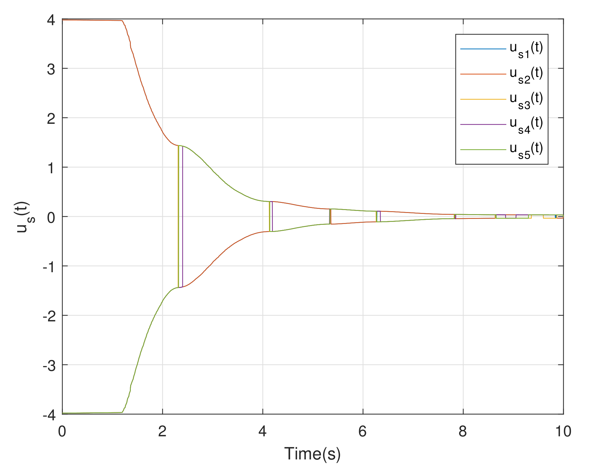
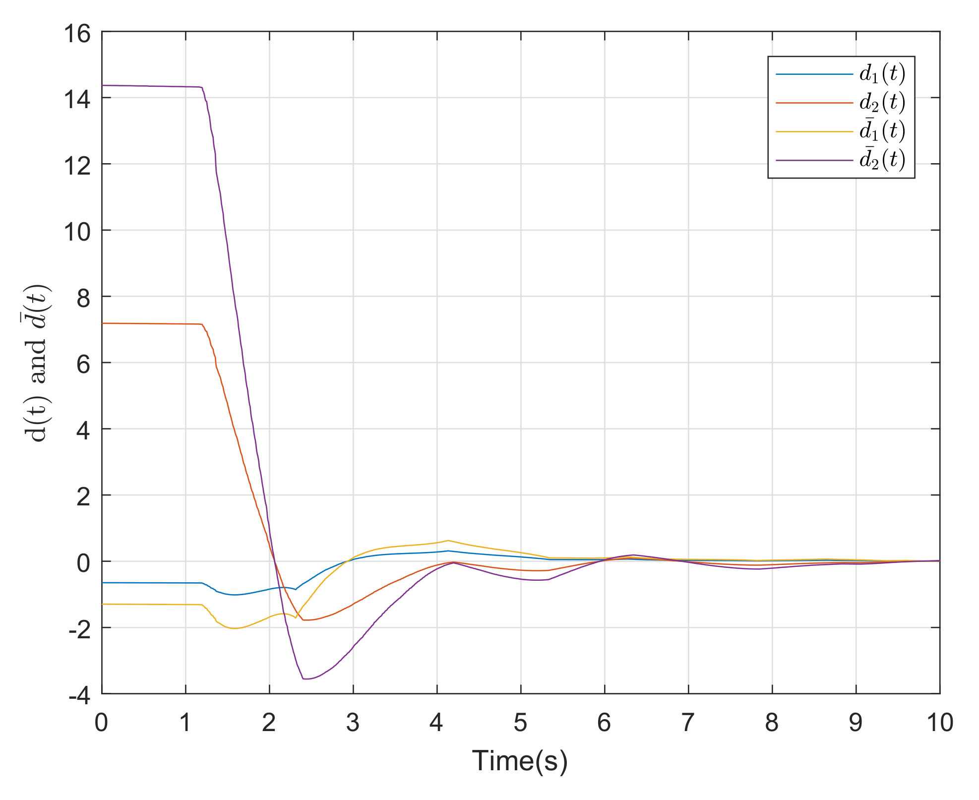
The simulation results for system (2) are shown in Figure 1, Figure 2, Figure 3, Figure 4, Figure 5 and Figure 6 below. The trajectory of error vector is shown in Figure 1. Figure 1 illustrates a comparison between the actual state of the system and the state estimated by the observer, and the error is asymptotically stable. The trajectories of output error sliding surface and discontinuous term are shown in Figure 2 and Figure 3, respectively. As shown in Figure 4, the state of the system is asymptotically stable, thus verifying that the sliding surface and controller are effective. It can be seen from Figure 3 that the system can reach the sliding surface in a short time, which is basically consistent with the theoretical analysis. The sliding variables (40) and the sliding mode controllers (59) are very close to zero after 8s. The comparisons of state vector , external disturbance , and sensor fault and their estimations are illustrated in Figure 4, Figure 5 and Figure 6, respectively. It can be seen that the proposed FTC approach can ensure the asymptotical stability of the closed-loop fault system.
The study in [44] investigates an adaptive fuzzy output feedback fault-tolerant optimal control problem for a class of single-input and single-output nonlinear systems. The comparison of the performance of the two controllers is given in Table 1 using the same data of Example. By comparison, it can be found that our method is better than the adaptive fuzzy sliding-mode controller (59) in terms of convergence time and steady-state error.
5. Conclusions
In this study, the adaptive fuzzy FTC problem was addressed for a class of nonlinear systems with actuator fault, sensor fault, and external disturbance. By augmenting the original plant into a normal system, a new SMO was designed to obtain the estimation of the state vectors and faults information. Based on the state estimation, an integral-type SMC strategy was developed to stabilize the closed-loop fault system. The advantage of this study is providing an observer that can simultaneously estimate state vectors, sensor faults, and external disturbances and has a wider estimation range than the traditional SMO. In addition, the effect of the time-varying actuator degradation in the error system can be eliminated because of the structure of the observer. However, there are some limitations in this article. For example, the proposed method is complicated in practical application and cannot be directly applied to descriptor systems. Future work will focus on extending the designed methods (small-gain theorem [44,45]) to more complicated systems such as switched systems and stochastic systems.
Author Contributions
Writing—original draft preparation, Y.N.; Writing—review and editing, Y.Z. and L.C. All authors have read and agreed to the published version of the manuscript.
Funding
This research was funded by the National Natural Science Foundation of China (No. 62003111, No. 61673099).
Institutional Review Board Statement
Not applicable.
Informed Consent Statement
Not applicable.
Data Availability Statement
The data used to support the findings of this study are obtained directly from the simulation by the authors.
Acknowledgments
This work is supported by the National Natural Science Foundation of China under Grant 61673099.
Conflicts of Interest
The authors declare no conflict of interest.
References
- Gao, Z.; Ding, S.X. State and Disturbance Estimator for Time-Delay Systems With Application to Fault Estimation and Signal Compensation. IEEE Trans. Signal Process. 2007, 55, 5541–5551. [Google Scholar]
- Wu, L.; Ho, D.W. Fuzzy filter design for Itô stochastic systems with application to sensor fault detection. IEEE Trans. Fuzzy Syst. 2009, 17, 233–242. [Google Scholar]
- Liu, X.; Gao, Z.; Chen, M.Z. Takagi-Sugeno Fuzzy Model Based Fault Estimation and Signal Compensation with Application to Wind Turbines. IEEE Trans. Ind. Electron. 2017, 64, 5678–5689. [Google Scholar] [CrossRef]
- Liu, X.; Gao, Z. Integrated fault estimation and fault-tolerant control for stochastic systems with Brownian motions. Int. J. Robust Nonlinear Control 2018, 28, 1915–1941. [Google Scholar] [CrossRef]
- Liu, X.; Han, J.; Wei, X.; Zhang, H.; Hu, X. Intermediate variable observer based fault estimation and fault-tolerant control for nonlinear stochastic system with exogenous disturbance. J. Frankl. Inst. 2020, 357, 5380–5401. [Google Scholar] [CrossRef]
- Zhang, K.; Jiang, B.; Staroswiecki, M. Dynamic output feedback-fault tolerant controller design for Takagi–Sugeno fuzzy systems with actuator faults. IEEE Trans. Fuzzy Syst. 2010, 18, 194–201. [Google Scholar] [CrossRef]
- Wang, X.; Yang, G.H. Fault-Tolerant Consensus Tracking Control for Linear Multiagent Systems Under Switching Directed Network. IEEE Trans. Cybern. 2020, 50, 1921–1930. [Google Scholar] [CrossRef]
- Li, Y.; Sun, K.; Tong, S. Observer-Based Adaptive Fuzzy Fault-Tolerant Optimal Control for SISO Nonlinear Systems. IEEE Trans. Cybern. 2019, 49, 649–661. [Google Scholar] [CrossRef]
- Tariq, M.F.; Khan, A.Q.; Abid, M.; Mustafa, G. Data-Driven Robust Fault Detection and Isolation of Three-Phase Induction Motor. Automatica 2019, 66, 4707–4715. [Google Scholar] [CrossRef]
- Deng, C.; Yang, G.H. Distributed adaptive fault-tolerant control approach to cooperative output regulation for linear multi-agent systems. Automatica 2019, 103, 62–68. [Google Scholar] [CrossRef]
- Yang, H.; Yin, S. Reduced order sliding mode observer-based fault estimation for Markov jump systems. IEEE Trans Autom. Control 2019, 64, 4733–4740. [Google Scholar] [CrossRef]
- Jiang, B.; Zhang, K.; Shi, P. Integrated fault estimation and accommodation design for discrete-time Takagi-Sugeno fuzzy systems with actuator faults. IEEE Trans. Fuzzy Syst. 2011, 19, 291–304. [Google Scholar] [CrossRef] [Green Version]
- Allahverdi, F.; Ramezani, A.; Forouzanfar, M. Sensor fault detection and isolation for a class of uncertain nonlinear system using sliding mode observers. Automatica 2020, 61, 219–228. [Google Scholar] [CrossRef]
- Li, Z.; Chen, X. Adaptive actuator fault compensation and disturbance rejection scheme for spacecraft. Int. J. Control Autom. Syst. 2021, 357, 5380–5401. [Google Scholar]
- Casavola, A.; Famularo, D.; Franzè, G. A robust deconvolution scheme for fault detection and isolation of uncertain linear systems: An LMI approach. Automatica 2005, 41, 1463–1472. [Google Scholar] [CrossRef]
- Karimi, H.R. Robust synchronization and fault detection of uncertain master-slave systems with mixed time-varying delays and nonlinear perturbations. Int. J. Control Autom. Syst. 2011, 9, 671–680. [Google Scholar] [CrossRef] [Green Version]
- Lin, B.; Su, X.; Li, X. Fuzzy Sliding Mode Control for Active Suspension System with Proportional Differential Sliding Mode Observer: Fuzzy SMC for active suspension system with PD sliding mode observer. Asian J. Control 2019, 21, 264–276. [Google Scholar] [CrossRef] [Green Version]
- Piltan, F.; Prosvirin, A.E.; Jeong, I.; Im, K.; Kim, J.M. Rolling-element bearing fault diagnosis using advanced machine learning-based observer. Appl. Sci. 2019, 9, 5404. [Google Scholar] [CrossRef] [Green Version]
- Zheng, W.; Xia, B.; Wang, W.; Lai, Y.; Wang, M.; Wang, H. State of charge estimation for power lithium-Ion battery using a fuzzy logic sliding mode Observer. Energies 2019, 12, 2491. [Google Scholar] [CrossRef] [Green Version]
- Xu, W.; Qu, S.; Zhao, L.; Zhang, H. An improved adaptive sliding mode observer for middle- and high-speed rotor tracking. IEEE Trans. Power Electron. 2009, 36, 1043–1053. [Google Scholar] [CrossRef]
- Gong, C.; Hu, Y.; Gao, J.; Wang, Y.; Yan, L. An improved delay-suppressed sliding mode observer for sensorless vector-controlled PMSM. IEEE Trans. Ind. Electron. 2019, 67, 5913–5923. [Google Scholar] [CrossRef]
- Cai, W.; She, J.; Wu, M.; Ohyama, Y. Disturbance suppression for quadrotor UAV using sliding-mode-observer-based equivalent-input-disturbance approach. ISA Trans. 2019, 92, 286–297. [Google Scholar] [CrossRef] [PubMed]
- Lopac, N.; Bulic, N.; Vrkic, N. Sliding mode observer-based load angle estimation for salient-pole wound rotor synchronous generators. Energies 2019, 12, 1609. [Google Scholar] [CrossRef] [Green Version]
- Chen, S.; Zhang, X.; Wu, X.; Tan, G.; Chen, X. Sensorless control for IPMSM based on adaptive super-twisting sliding-mode observer and improved phase-locked loop. Energies 2019, 12, 1225. [Google Scholar] [CrossRef] [Green Version]
- Xiong, Y.; Saif, M. Sliding mode observer for nonlinear uncertain systems. IEEE Trans. Autom. Control 2001, 46, 2012–2017. [Google Scholar] [CrossRef]
- Apaza-Perez, W.A.; Moreno, J.A.; Fridman, L. Global Sliding Mode Observers for Some Uncertain Mechanical Systems. IEEE Trans. Autom. Control 2020, 65, 1348–1355. [Google Scholar] [CrossRef]
- Li, J.; Yang, G.H. Fuzzy Descriptor Sliding Mode Observer Design: A Canonical Form-Based Method. IEEE Trans. Fuzzy Syst. 2020, 28, 2048–2062. [Google Scholar] [CrossRef]
- Nguyen, N.P.; Hong, S.K. Fault diagnosis and fault-tolerant control scheme for quadcopter UAVs with a total loss of actuator. Energies 2019, 12, 1139. [Google Scholar] [CrossRef] [Green Version]
- Huang, S.N.; Tan, K.K. Fault detection, isolation, and accommodation control in robotic systems. IEEE Trans. Autom. Sci. Eng. 2008, 5, 480–489. [Google Scholar] [CrossRef]
- Aslam, M.S.; Ullah, R.; Dai, X.; Sheng, A. Event-triggered scheme for fault detection and isolation of non-linear system with time-varying delay. IET Control Theory Appl. 2020, 14, 2429–2438. [Google Scholar] [CrossRef]
- Li, H.; Gao, H.; Shi, P.; Zhao, X. Fault-tolerant control of Markovian jump stochastic systems via the augmented sliding mode observer approach. Automatica 2014, 50, 1825–1834. [Google Scholar] [CrossRef]
- Liu, M.; Shi, P. Sensor fault estimation and tolerant control for Itô stochastic systems with a descriptor sliding mode approach. Automatica 2013, 49, 1242–1250. [Google Scholar] [CrossRef]
- Jin, Z.; Wang, Z.; Li, J. Input-to-state stability of the nonlinear fuzzy systems via small-gain theorem and decentralized sliding mode control. IEEE Trans. Fuzzy Syst. 2021. [Google Scholar] [CrossRef]
- Zhang, Y.; Jin, Z.; Zhang, Q. Impulse elimination of the Takagi-Sugeno fuzzy singular system via sliding mode control. IEEE Trans. Fuzzy Syst. 2021. [Google Scholar] [CrossRef]
- Hou, H.; Yu, X.; Xu, L.; Rsetam, K.; Cao, Z. Finite-time continuous terminal sliding mode control of servo motor systems. IEEE Trans. Ind. Electron. 2020, 67, 5647–5656. [Google Scholar] [CrossRef]
- Hou, H.; Yu, X.; Fu, Z. Sliding-mode control of uncertain time-varying systems with state delays: A non-negative constraints approach. IEEE Trans. Syst. Man Cybern. Syst. 2020. [Google Scholar] [CrossRef]
- Hou, H.; Yu, X.; Xu, L.; Chuei, R.; Cao, Z. Discrete-time terminal sliding-mode tracking control with alleviated chattering. IEEE/ASME Trans. Mechatron. 2019, 24, 1808–1817. [Google Scholar] [CrossRef]
- Qian, M.; Yi, H.; Zheng, Z. Integrated fault tolerant attitude control approach for satellite attitude system with sensor faults. Optim. Control Appl. Methods 2020, 41, 555–570. [Google Scholar] [CrossRef]
- Mallavalli, S.; Fekih, A. A fault tolerant tracking control for a quadrotor UAV subject to simultaneous actuator faults and exogenous disturbances. Int. J. Control 2020, 99, 655–668. [Google Scholar] [CrossRef]
- Chen, C.P.; Liu, Y.J.; Wen, G.X. Fuzzy Neural Network-Based Adaptive Control for a Class of Uncertain Nonlinear Stochastic Systems. IEEE Trans. Cybern. 2014, 44, 583–593. [Google Scholar] [CrossRef] [PubMed]
- Feng, X.; Wang, Y. Fault estimation based on sliding mode observer for Takagi-Sugeno fuzzy systems with digital communication constraints. J. Frankl. Inst. 2020, 357, 569–588. [Google Scholar] [CrossRef]
- Richiedei, D.; Tamellin, I. Active control of linear vibrating systems for antiresonance assignment with regional pole placement. J. Sound Vib. 2021, 494, 115858. [Google Scholar] [CrossRef]
- Faria, F.A.; Assunção, E.; Teixeira, M.C.; Cardim, R.; Da Silva, N.A.P. Robust state-derivative pole placement LMI-based designs for linear systems. Int. J. Control 2009, 82, 1–12. [Google Scholar] [CrossRef]
- Jin, Z.; Wang, Z. Input-to-state stability of the nonlinear singular systems via small-gain theorem. Appl. Mathe. Comput. 2020, 402, 126171. [Google Scholar] [CrossRef]
- Liu, T.; Jiang, Z.P. A small-gain approach to robust event-triggered control of nonlinear systems. IEEE Trans. Autom. Control 2015, 60, 2072–2085. [Google Scholar] [CrossRef]
Figure 1.
Trajectories of .

Figure 2.
Trajectories of .

Figure 3.
The discontinuous input .

Figure 4.
and its estimation.

Figure 5.
and its estimation.

Figure 6.
and its estimation.


Table 1.
The performance indexes of our method and [8].
Publisher’s Note: MDPI stays neutral with regard to jurisdictional claims in published maps and institutional affiliations. |
© 2021 by the authors. Licensee MDPI, Basel, Switzerland. This article is an open access article distributed under the terms and conditions of the Creative Commons Attribution (CC BY) license (https://creativecommons.org/licenses/by/4.0/).
Share and Cite
MDPI and ACS Style
Zhang, Y.; Nie, Y.; Chen, L. Adaptive Fuzzy Fault-Tolerant Control against Time-Varying Faults via a New Sliding Mode Observer Method. Symmetry 2021, 13, 1615. https://0-doi-org.brum.beds.ac.uk/10.3390/sym13091615
AMA Style
Zhang Y, Nie Y, Chen L. Adaptive Fuzzy Fault-Tolerant Control against Time-Varying Faults via a New Sliding Mode Observer Method. Symmetry. 2021; 13(9):1615. https://0-doi-org.brum.beds.ac.uk/10.3390/sym13091615
Chicago/Turabian StyleZhang, Yi, Yingying Nie, and Liheng Chen. 2021. "Adaptive Fuzzy Fault-Tolerant Control against Time-Varying Faults via a New Sliding Mode Observer Method" Symmetry 13, no. 9: 1615. https://0-doi-org.brum.beds.ac.uk/10.3390/sym13091615
Note that from the first issue of 2016, this journal uses article numbers instead of page numbers. See further details here.