
Unified Theory of Unsteady Planar Laminar Flow in the Presence of Arbitrary Pressure Gradients and Boundary Movement


1
Department of Aviation, Minnesota State University, Mankato, MN 56001, USA
2
AAR Aerospace Consulting, L.L.C., Saint Peter, MN 56082, USA
Symmetry 2022, 14(4), 757; https://0-doi-org.brum.beds.ac.uk/10.3390/sym14040757
Submission received: 19 February 2022
/
Revised: 27 March 2022
/
Accepted: 31 March 2022
/
Published: 6 April 2022
(This article belongs to the Special Issue Symmetry in Fluid Flow II)
Abstract
:A general unified solution of the plane Couette–Poiseuille–Stokes–Womersley incompressible linear fluid flow in a slit in the presence of oscillatory pressure gradients with periodic synchronous vibrating boundaries is presented. Oscillatory flow remains stable and laminar with no-slip boundary conditions applied. Eigenfunction expansion method is used to obtain the exact analytical solution of the general linear inhomogeneous boundary value problem. Fourier expansion of arbitrary harmonic pressure gradient and non-harmonic wall oscillations was used to calculate arbitrary driving of the fluid. In-house developed optimized computational fluid dynamics marching-in-time finite-volume method was used to test and verify all analytical results. A number of particular transients, steady-state and combined flows were obtained from the general analytical result. Generalized Stokes and Womersley flows were solved using the analytical computations and numerical experiments. The combined effects of periodic non-harmonic wall movements with oscillatory pressure gradients offers rich and interesting flow patterns even for a linear Newtonian fluid and may be particularly interesting for pumping-assist microfluidic devices. The main motivation for developing a unified solution of the unsteady laminar planar Couette–Stokes–Poiseuille–Womersley flow originates in a need for, but is not limited to, in-depth exploration of flow patterns in hemodynamic and microfluidic pumping applications.
1. Introduction
The solutions of the classical fully-developed steady laminar flows, such as the planar Couette (CT) and the planar Poiseuille (PO) flows in an infinite slit, have been known for a long time [1,2,3,4,5,6,7,8,9]. The Couette flow originates in a fluid motion between two coaxial cylinders and is shear-driven (wall-driven). If the radii of the cylinders are large, then planar CT flow is approximated. On the other hand, PO flow is solely pressure-driven. A planar steady-state Couette–Poiseuille (CP) flow is a linear combination of the CT flow with one boundary moving at uniform speed and the PO flow between two fixed infinite plates caused by the steady-state (proverse or adverse) pressure gradients (PG). These classic solutions of the formidable nonlinear Navier–Stokes (N-S) equations also paved the way to early investigation of the flow stability and transition to turbulence [2,5,10]. The Womersley (WO) flow that can be seen as a generalization of the PO flow is pressure-driven caused by oscillating PGs with fixed conduit boundaries. Such flows have also been known for quite some time [4,5,7,11,12,13,14,15] and often under different names too. WO-type flow has important applications in pulsatile arterial hemodynamics and many biological fluid systems [15,16,17].
Unsteady shear-driven flows with moving boundaries were first tackled with, so-called, Stokes’ (ST) 1st and 2nd problem [1,4,5]. Stokes’ 1st problem (ST1) treats flow transients after a single infinite flat plate is suddenly set in uniform motion. A fluid then asymptotically settles into the steady-state (Couette-like) flow after decay of initial transients. Stokes’ 2nd problem (ST2) treats the harmonically vibrating infinite flat plate problem that sets still semi-infinite fluid in oscillatory motion. The quasi-steady-state (QSS) flow oscillations take place after the initial transients are attenuated. A fluid closer to the moving boundary will be more affected by the oscillating wall due to viscous diffusivity, which is chiefly responsible for the decaying transfer of the linear momentum deeper into the fluid mass [17,18,19]. Stokes’ 2nd problem (ST2) is in many respects similar to Kelvin’s problem of penetration of harmonically induced temperature waves into the semi-infinite (soil) medium. Carslaw and Jaeger [20] provide detailed analytical solutions and discussion of this important problem. Thus, ST (ST1 and ST2) and WO flows are by nature unsteady, while CT and PO flows are steady flows.
Numerous experiments have confirmed the validity and theoretical soundness of these particular basic flows. The general validity of the N-S equations in continuum hydrodynamic approximation has also been confirmed in numerous experiments. The question of the molecular, apparent, or effective slip at the liquid–solid boundary is still open and a topic of intense current research activities. Although based on an entirely different concept, the Lattice Boltzmann Method (LBM) originating in mesoscopic consideration of the particle density function on symmetry-preserving lattice including streaming and collision operators have also confirmed the general validity of the incompressible N-S equations in a low-Mach number LBM limit [21,22,23,24]. The continuum fluid behavior has also been confirmed by the Molecular Dynamic (MD) and Metropolis Monte Carlo (MMC) simulations on a true microscopic (particle) scale involving Hamiltonian of atomic and molecular interactions [25,26,27,28,29]. At very small length scales, microscales for gases and nanoscales for liquids, we do however expect departure from the continuum N-S equations [30,31].
The basic flow models mentioned above have been already used on many occasions in modeling hemodynamic flow and cardiovascular circulation. Early measurements by McDonald [32] and Hale et al. [33] were supported by theoretical considerations of oscillatory pressure-driven flows in elastic tubes by Womersley [34,35]. A good review of blood flow phenomena in arteries was presented in [36]. Daidzic [17] successfully used the Womersley flow model to smooth out velocity profiles and recover oscillatory shear stress information lost during multi-gate Doppler ultrasound measurements of blood mimicking fluid in blood-vessel-type conduits. Additionally, very recently, Giusti and Mainardi [37] studied viscoelastic fluid effects in fluid-filled elastic tubes. Although it was suspected for a long time, it was actually only quite lately shown experimentally that the longitudinal motion of blood vessel walls exists due to wall shear [38] on the blood vessel interface.
The main goal of this research article is to present a unified theory of laminar Newtonian fluid flows with moving boundaries (shear-driven) and unsteady PGs (pressure-driven) for the combined planar CT, PO, ST, and WO, or as termed here, a planar Couette–Poiseuille–Stokes–Womersley (CPSW) flow. Flow is generated in planar (slit) geometry between two infinite rigid impenetrable flat plates. Since the walls are parallel and impermeable only the axial velocity component remains. Interaction of forced wall oscillations and applied unsteady PGs results in interesting transient and QSS flow patterns. Specifically, non-harmonic shear and/or pressure forces for linear fluid are discussed for the first time in a consistent and in-depth manner to the best of our knowledge. In many instances the hemodynamic flows can be approximated with a Newtonian fluid and so this theoretical numerical analysis is directly applicable. One of the important applications of the findings from this study is in the utilization of shear-driven flows and the design of micropumps.
2. Mathematical Model
Within the realm of continuum hydrodynamics, the N-S equations will be used as a starting point to describe an unsteady motion of the Newtonian fluid. The flow is incompressible and divergence-free. The oscillatory non-harmonic synchro-phased periodic motion of two solid interfaces in a slit geometry will be modeled using the Fourier expansion of the arbitrary periodic excitation waveforms. The PGs are modeled by assuming an infinite pressure disturbances group speed and will thus be time-dependent only [8].
We made few important assumptions: fluid behavior is incompressible, linear, and time-independent (no internal dynamics) where viscosity is shear- and temperature-independent, flow remains laminar and isothermal at all times, entrance effects are neglected, boundary walls are rigid and impenetrable, Dirichlet no-slip BCs exist, periodic oscillations of boundary movement and PGs and hyperbolic effects are neglected. The IBVP discussed here is well-posed [39,40].
2.1. Fluid Flow Model
The general 3D unsteady conservation equations for mass, momentum, and energy for a linear compressible fluid in conventional tensor and vector notation and Cartesian coordinates [2,5] yields:
We can regard Equation (1) as a sort of “standard model” of continuum (low-Knudsen number) fluid mechanics. The N-S equations and the thermal energy equation are essentially phenomenological as the linear fluid stress–strain rate and the heat conduction relationships are semi-empirical. Generally, for Newtonian (linear) fluids, we may write:
where for conservative forces:
and:
The viscous dissipation function is a non-negative expression of the irreversible flow energy conversion into heat due to deviatoric part of the stress tensor [2,5]:
Typically, it is assumed that the bulk viscosity vanishes (Stokes hypothesis). Additionally, if the flow is incompressible, the second-viscosity term vanishes identically and all is left from the deviatoric part of the stress tensor is the deformation tensor .
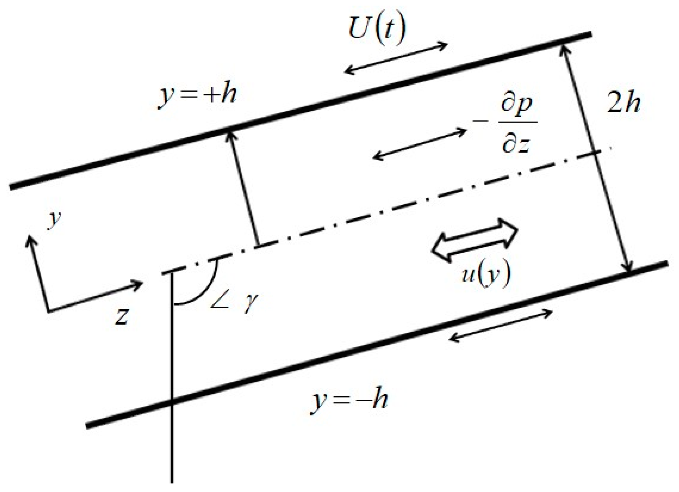
A Newtonian incompressible fluid in an unsteady laminar fully developed flow with oscillatory PG components and both walls vibrating periodically in plane slit geometry is investigated. Both the PGs and the wall motion may oscillate in an arbitrary periodic fashion (ST2). A schematic of the flow geometry is illustrated in Figure 1. Other than gravity, no other body forces are assumed to be acting.
The unsteady fully developed isothermal laminar flow in an infinite slit geometry with no-slip BCs and incompressible Newtonian (linear) fluid can thus be reduced to the following IBVP:
The auxiliary conditions are:
The BCs are split into the steady-state part due to uniform wall motion (CT component) and an arbitrary periodic wall oscillation (ST component) described by the appropriate complex Fourier series. Similarly, the PGs consist of the steady-state (PO) component superposed onto a linear combination of many (WO) harmonic components. The phasors of the PGs are complex numbers which contain amplitude (modulus) and phase (argument) information:
The steady-state (static) part of the PG includes gravity component:
Although the real-valued steady-state externally applied PG and the DC-value, or average-value, zero-order Fourier coefficient have different origins they can be lumped together.
Expressions for oscillating PGs and wall movement are conveniently given in a complex form greatly simplifying theoretical analysis. All periodic functions for the PGs and the BCs are real-valued, thus possessing conjugate symmetry, () [39,40,41,42]. The complex Fourier series can be converted into the classical or the phase form for an arbitrary function:
where:
The complex Fourier coefficients are calculated using the inherent orthogonal property of conjugate complex exponentials:
It is convenient to express the complex Fourier coefficients as phasors where the modulus is , and the phase satisfies . The complex Fourier series now yields:
One must be careful when calculating the phase constant. All quadrants must be inspected as the inverse tangent is not a single-valued function. The modulus of the complex Fourier coefficient must be a real non-negative number. The complex Fourier coefficients carry the information from both, the real and the imaginary, part if the function is neither even nor odd (). For an even real-valued function, (), while for an odd real-valued function, , , and, . Any function can be represented as the sum of respective even and odd functions. In the case of non-harmonic periodic wall oscillations, the Fourier series will necessarily contain both, real and imaginary, components.
Due to the mass conservation the only velocity component surviving is the longitudinal (axial) along the conduit axis. Due to the divergence-free flow, the second-viscosity term disappears identically from the general strain rate expression (bulk viscosity is zero) without the need to invoke Stokes’ hypothesis. Although we calculate dissipation function, the energy equation is not solved explicitly as the flow is enforced to remain isothermal. Alteration of physical properties due to temperature changes are thus neglected and difficult nonlinear coupled problem is avoided. As the slit thickness is small, the gravity plays no significant role in the lateral direction and the pressure is uniformly distributed in each cross-section. However, the gravitational potential may be important for driving flows in non-horizontal slits.
2.2. Dimensional Form of the IBVP
The main IVBP in compact dimensional form yields:
The expression for PG source function (only time dependent here but we keep spatial dependence for generality), is:
Additionally, for BCs:
In the case of the periodic wall motion, there will be no Couette velocity components (). In the case of an odd wall-driving function, the (Stokes’ component) DC-value will be zero. In the case of an even function, a non-vanishing velocity DC-component can be regarded as a standalone steady-state value. The ICs are general and an arbitrary velocity distribution at time zero can be specified.
2.3. Nondimensional form of the IBVP
Transforming general CPSW flow into dimensionless form is difficult. There are several choices of the characteristic velocity [5,7]. In the case of the classic CT flow, the plate’s uniform velocity is the characteristic velocity and could never be exceeded in the flow field. For a planar PO flow, the maximum velocity in the center of the parabolic profile which is a function of the uniform PG can be used as a characteristic velocity. For the oscillatory PG (WO-component) we could use amplitude and frequency of any harmonic as a characteristic velocity. It is recommended to use the one with the largest magnitude [7] to ensure range [0, 1], but that is not always possible. Let us now define new dimensionless variables:
The velocity scaling will change depending on the particular flow situation, i.e., presence of the wall movement or steady and/or dynamic PGs. The characteristic velocity could be uniform wall velocity, maximum plane PO velocity in the slit centerline or the mth-harmonic WO velocity caused by respective dynamic PG oscillations:
One can now define a Womersley (WO) number which is often also referred to as the “Witzig” number [37] or the “kinetic Reynolds” number (square of the WO number) [2,5,7]:
The WO-number, , has a very specific physical meaning and can be thought of as the ratio of the half channel height versus Stokes’ or viscous penetration layer. For example, due to wall oscillations the momentum (or more appropriately—vorticity) is being diffused. The ensuing pseudo “shear-waves” are purely dissipative (and dispersive) and attenuate exponentially with distance from the solid vorticity-generating surfaces. Alternatively, we may think of the WO number as the ratio of times due to diffusion and oscillation or as the ratio of velocities due to oscillations and viscous momentum diffusion:
A very high WO number (>10) would in this case mean that the lateral channel dimension is much larger than the zone of influence (radius of action) of the moving surface and that the bulk of the fluid will not “feel” its presence:
For small WO numbers, the viscous penetration layer extends practically instantly over the entire lateral flow domain and diffusion is rapid compared to slow wall oscillations. In this case, we have a sort of quasi-steady-state planar PO flow where the fluid follows the slow boundary motion with vanishing phase lag. Hence, we arrive at the quasi-equilibrium solutions:
By using the dimensionless variables, defined in Equation (13), and substituting them into Equations ((10)–(12)), we obtain the non-dimensional IBVP:
with
where:
The asterisk here refers to dimensionless and not the complex conjugate values. In order to avoid cluttering the symbols and equations we are going to intentionally omit asterisk superscript for dimensionless quantities in subsequent derivations.
2.4. Boundary Conditions and Stability of Pulsatile Flows
The question of Dirichlet’s no-slip BCs for velocity in micro-fluidic flows of similar geometry has already been thoroughly discussed in [18]. Additionally, the general mixed BCs often referred to as Robin BCs for fluid velocity can be expressed as in the case of partial slip:
where Ls is Navier–Maxwell slip length. Here, we have assumed full no-slip condition in both forward and return wall motion and the Robin BC boils down to Dirichlet BC.
The classical linear stability theory [2,4,5,6,10] predicts absolute stability for steady planar CT and PO flows in rigid tubes, i.e., entirely contrary to experimental evidence. On the other hand, plane PO flow has critical Reynolds number of about 5750 obtained by solving the Orr-Sommerfeld equation [2,4,5,6,10]. Experimentally, the first Tollmien–Schlichting (TS) wave appears, and the onset of flow transition occurs at Reynolds numbers as low as 360. The stability of pulsatile flows in cylindrical and plane geometries is of equal importance and is gaining more importance for microfluidic applications. The science of the flow stability is vast and cannot be treated here in any detail. It suffices to say that the maximum Reynolds number occurring in our analysis stays well below the critical and the assumption of an all-time laminar flow thus seems appropriate.
3. Methods and Materials
To obtain the closed-form analytical solution of this linear non-homogeneous IBVP problem we use the powerful method of eigenfunction expansion (EEM) [39,40,41,42,43]. The entire linear non-homogeneous IBVP problem can be treated directly by EEM. However, in order to arrive at a general solution in a physically more transparent way we will decompose the velocity field into a steady-state, transient and quasi-steady-state (QSS). This is permissible as the governing PDE is linear and the general principle of linear superposition applies. Keeping in mind that all variables are dimensionless, we can write for the velocity field:
The first component on the RHS is the steady CP flow that may also contain DC PG components from the respective Fourier expansions. The 2nd term represents transient response to ICs and will vanish after the finite amount of time (rapidly in most cases). The 3rd velocity component represents the QSS velocity field (ST-WO component) as a response to arbitrary non-harmonic boundary motion and unsteady PG. However, the third component may also contain some transient responses due to phase information contained in the Fourier expansions.
To solve resulting IBVPs by EEM we invoke the formidable and well-developed mathematical apparatus of self-adjoint linear operators in infinite-dimensional separable Hilbert function space [44,45,46,47,48] (or L2-metric space in particular). It is the same theoretical basis that lies at the mathematical foundation of the quantum mechanics. The eigenfunctions of the self-adjoint (Hermitian) linear differential operator in Hilbert space form a closed and complete basis set and are used in generalized Fourier series expansions.
3.1. Solution of the Steady-State BVP
The first BVP defines steady CP flow and is described in a dimensionless form as:
The solutions for the dimensionless velocity field, flow rate, velocity gradient, tangential stress, vorticity, and dissipation () are:
In general CP flow, the uniform wall velocity (of a faster moving wall) is used to obtain the dimensionless form and the non-dimensional PG can assume any value (). Clearly, a plethora of uniform wall movements in combination with a choice of static (proverse or adverse) PGs are possible.
If bounding infinite walls are immovable, we obtain the classical plane PO flow, , with, . In the plane PO flow, the wall velocity is zero and cannot be used for scaling purposes. Therefore, the characteristic velocity is the maximum velocity in the center and dimensionless PG must be , in accordance with Equations (13) and (14).
3.2. Solution of the Homogeneous IBVP
An infinite-dimensional Hilbert space is an inner-product separable normed metric space with definite algebra and topology. Completeness of eigenfunctions in L2 or Hilbert space is guaranteed by, often called, Parseval’s equality [39,40,41,42,43] which forms the equivalence part of the Bessel’s inequality and represents energy conservation principle (completeness of eigenfunctions). The L2 or mean-square convergence is automatically assured for complete basis sets only requiring that the function is square-integrable in the Lebesgue integral (absolute) sense or is Lebesgue-measurable [44,45,46,47,48,49,50]:
The mathematical apparatus of functional analysis and L2 space used here is based on the celebrated Riesz–Fisher theorem [44,45,46,47] which establishes the isomorphism of vector space l2 and function space L2 as Hilbert spaces. Assuming a complete basis set of eigenfunctions, a Lebesgue square-integrable function (vast majority also Riemann-integrable) can be represented as a linear combination of orthonormal eigenfunctions:
where the generalized Fourier coefficients follow from orthogonality:
The second problem is a simple homogeneous IBVP with modified ICs originating due to steady-state CP flow:
This is a parabolic PDE problem that can be solved using the SOV [31,32,33,34] method (sometimes also called Fourier method). The solution of the simple Sturm–Liouville () BVP is:
The cosine eigenfunction would be a solution of the BVP if the flow is symmetric (BCs are identical or periodic). The eigenvalues (zeros) of the cosine eigenfunctions are:
However, when problems are asymmetric, we need both cosine and sine eigenfunctions appearing alternatively and with changing signs. The general asymmetric solution can be thus represented by the following eigenvalues and eigenfunctions:
This eigenfunction is basically a sum of cosine and sine eigenfunctions appearing alternatively in infinite sums. All eigenvalues here must be non-negative real numbers as required by the regular Sturm–Liouville (S-L) theory [39,40,41,42,43,51,52,53,54]. Classical Fourier series are only one of the infinitely many possible complete eigenfunction basis sets.
We mostly treat symmetric flows here with cosine eigenfunctions, describing a complete basis set of normalized and orthogonal (orthonormal) eigenfunctions:
We have not yet stated ICs explicitly. For example, a PO parabolic velocity profile in a slit could be used for studying stopping (shutdown) flow dynamics. For simplicity and to obtain fast closed-form solutions, we assume uniform velocity profiles only (say, zero or one):
The Fourier coefficients of the 2nd IBVP are now:
The complete solution of the symmetric (decaying) transient flow is a linear superposition involving several ICs:
The first term in the above Fourier expansion describes the effect of the initial velocity distribution. The second term gives transients due to sudden application of the constant PG, while the third component is the response to the sudden instant finite uniform movement (ST1 problem) of the upper and/or lower infinite plate at time zero. Negative exponential factor ensures decaying flow with higher flow harmonics diminishing more rapidly. Starting and stopping flow transients can be deduced from the general solution here.
3.3. Solution of the Non-Homogeneous IBVP for Symmetric Flows
The third and final IBVP problem which has both inhomogeneous PDE and BCs.
Both arbitrary, yet periodic, BCs and the pressure source term are given in terms of complex Fourier coefficients. We can always find a suitable (shifting) function that will satisfy the non-homogeneous BCs [19,31,32,33,34,35]. In this way we obtain homogeneous BCs, but the new PDE often ends up with additional source terms. While this technique is perfectly good and often results in solutions containing uniformly convergent series in the entire domain, it is time consuming and problem specific. More general, elegant, and faster solutions are obtained by the straightforward use of EEM although we may get discontinuity at the boundaries thus invalidating uniform convergence in the entire domain. However, mean-square convergence is automatically assured due to the completeness of eigenfunctions. Other analytical methods, such as Laplace transform, Finite Fourier Transform, Green’s functions, etc., could be used to solve bounded non-homogenous problem [20,39,40,41,42,43].
The essence of the EEM is to tailor the inhomogeneous solution in terms of the orthonormal eigenfunctions φn(y) of the corresponding (associated) homogeneous BVP (CHBVP):
By utilizing the orthogonal property of the eigenfunctions and the norm, we obtain:
Using these relationships, the decomposed oscillating PG source term is:
One may think that all IC transients were taken care in the homogeneous IBVP (2nd problem), but that is not the case. Although the ICs are explicitly zero here, the initial information is also hidden in phasors. Therefore, we are dealing with the QSS response caused by periodic forcing functions and few transients caused by non-zero phases. Any transient due to sudden application of the oscillating PG will be taken care of in the solution of this non-homogeneous IBVP. With compatibility condition satisfied [42], the resulting Fourier series is uniformly convergent in the entire domain including boundaries.
Since the term-by-term differentiation is prohibited for the Fourier series that does not converge uniformly, when utilizing Green’s 2nd identity [39,40,41,42,43], one obtains:
Implementing the general solution of the inhomogeneous linear first-order ODE, we obtain:
The solution of the 3rd non-homogenous IBVP problem is thus:
After tedious complex algebra reductions, one obtains:
3.4. Global Solution for Symmetrically Driven Flows
A global solution of the symmetric IBVP is obtained by linearly superposing all three velocity components as given by Equation (19). After grouping all terms, the final dimensionless solution yields:
Phase and amplitudes (damping factors) of the oscillation response are:
The damping factors are positive-definite. Higher interface-motion harmonics will generate correspondingly higher Womersley (WO) numbers, , thus penetrating ever shallower into the fluid mass, but significantly affecting its phase lags. The solution consists of two traveling waves moving in the opposite directions, i.e., coming from each wall. Different regions of fluid are experiencing varying effects of resistance and inertia. Daidzic and Hossain [18] and Hossain and Daidzic [19] have demonstrated similar behavior for Newtonian and some shear-thinning non-Newtonian fluids.
An arbitrary periodic function can be represented by converging the Fourier series. At least an L2 or mean-square convergence is guaranteed for Lebesgue square-integrable functions:
Mean-square convergence does not imply pointwise or uniform convergence [39,40,41,42,43,51,52,53,54]. At the finite points of jump discontinuities of piecewise continuous functions, the Fourier series will converge to the average value of the left and the right limits with Gibbs phenomena and characteristic “ringing” appearing [39,40,41,42,43,51,52,53,54]. Accordingly, the convergence cannot possibly remain uniform. Once we have chosen oscillation waveforms, their Fourier coefficients can be directly substituted into the global solution (Equation (38)). The question of convergence is not the academic one. The nature of convergence strongly affects analytical solutions and computations. From the velocity distribution in the complex form, we can easily derive volume flow rate (VFR):
The velocity gradient of the axial velocity is:
A word of caution is required. Term-by-term differentiation of a Fourier series is a delicate matter effectively multiplying a series by a factor (n), slowing its convergence, and is only allowed if the series and differentiated series converges uniformly [51,52,53,54,55,56]. Term-by-term integration is usually a less critical issue as a multiplication factor (1/n) is introduced accelerating the convergence [51,52,53,54,55,56]. The classical Fourier series can always be integrated term-by-term [51,52,53,54,55,56].
3.5. Numerical Method
To verify theoretical solutions, we employ numerical experiments using in-house-developed CFD programs. The finite-volume method (FVM) to discretize N-S equations [57,58,59,60] and to numerically calculate the flow field was employed. FVM is in many respects similar to the FD method, but spatial-temporal discretization is obtained while assuring conservation of flow properties in every small finite volume. To verify the accuracy, stability, consistency, and efficiency of numerical models, we test our CFD against several well-known analytic solutions [18,19]. Despite known shortcomings, the conditionally stable explicit FTCS discretization works very well for the 1D flow case. The problem with the Crank–Nicolson (C-N) or the fully implicit methods is that we must solve the system of linear algebraic equations at each time step. Fortunately, for 1D flow an efficient tri-diagonal matrix solver utilizing Thomas’ (TDMA) Gauss-elimination algorithm is used [18,19,57,58,59,60]. For 2D and 3D flows, we have to employ different methodologies. While it is often stated that the implicit schemes are unconditionally stable that may be useless feature when the accuracy suffers due to excessively large time steps.
The solution of the linear parabolic PDE given in Equation (5) is quite simple and can be most rapidly obtained by marching in time while complying with given IC and BCs. An added feature of the FVM is that it automatically satisfies conservation laws as each balance differential equation is integrated over a small control (finite) volume. It also accounts for all source (volumetric) and surface interactions. The numerical methodology implemented here was already sufficiently described earlier [18,19] and we only repeat here the most essential parts.
The “old” values of velocity at grid points can be denoted by , and the updated values at the “new” time , can be denoted by . If we designate:
The spatial-temporal discretized equation yields:
where
Here, f stands for the time-approximation weighting factor with the range [0, 1]. The value of f will determine whether the discretization scheme is explicit, fully implicit or C-N. The unconditionally stable popular implicit C-N (CTCS) method () is second-order accurate, both, in time and space:
A simple explicit (FTCS) discretization with the time-dependent PG as a source function yields:
Appropriate IC and BCs must be applied for the numerical computations. By choosing the proper stability parameter λ(=1/4) we can, in fact, obtain second-order accuracy in time.
3.6. Modeling of Pressure Gradients
The most comprehensive planar CPSW problem treated here is the one that includes both the periodic non-harmonic oscillations of two boundary wall plates in concurrence with the applied oscillatory periodic PGs. We assume that both plates move simultaneously and in phase and thus the problem is symmetric. The oscillatory PG is superposed to a steady-state PG when applicable. Clearly an infinite number of combinations of wall and PG dynamics are possible.
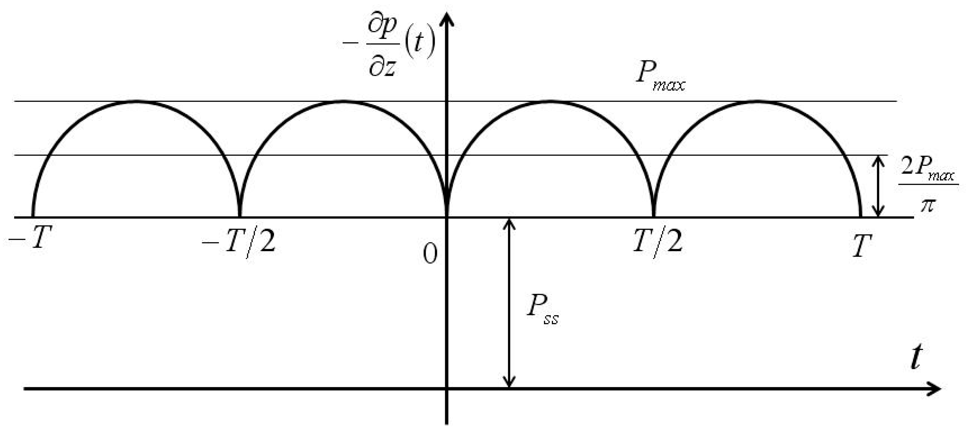
We chose a rectified-sine (absolute-sine) function to represent PG oscillatory dynamics. Another interesting choice of pressure oscillations would be in emulating heartbeat waveforms for pulsatile arterial hemodynamic applications. Digitally sampled waveforms can be utilized by employing harmonic analysis and calculating the Fourier coefficients of an arbitrary discrete excitation. A full-wave rectified-sine (absolute-sine) function delivering oscillating PGs on top of the steady-state PG for a horizontal slit is illustrated in Figure 2, and is described by:
This even real-valued function can be expressed in terms of Fourier cosine series. By using Euler formulas [39,40,41,42,43,51,52,53,54,55,56] for Fourier coefficients, one obtains:
It is easy to demonstrate, using the Weierstrass convergence M-test [40,41,42], that this Fourier series converges uniformly and accordingly pointwise as well. Function in Equation (46) is square-integrable and its Fourier series thus converges in the mean (L2 sense). This was already expected from the uniform convergence. Utilizing Parseval’s identity in the real form yields:
The convergence rate is relatively fast (1/n2) since the function is continuous and the first derivative is piecewise continuous. For a real-valued even rectified-sine waveform, An = A−n, and Bn = 0, one obtains:
In phasor form, the Fourier series yields the same result given in Equation (47) earlier:
The imaginary part of the complex Fourier coefficient is zero and the phase constant is π. Since the infinite series of squares of Fourier coefficients is bounded by the norm of the square-integrable function, the Riemann–Lebesgue lemma [44,45,46,47] assures us that:
Using Parseval’s (or Plancherel’s) identity in the complex form delivers the same result as with real form:
The first 20 harmonic terms are sufficient to approximate rectified-sine function with high accuracy as the function is smooth everywhere except for the first derivatives being discontinuous at the half-period points.
3.7. Modeling of Wall Oscillations
The uniform wall movement such as in the classic planar CT flow is not easy to achieve in practice and especially not on microscales. Net flow rate induced by non-harmonic oscillatory motion of Newtonian and non-Newtonian fluids in a slit and in the absence of PGs was treated numerically [18,19]. However, in the numerical analysis presented in [18,19], the return stroke was assumed to be so fast that full slip occurred. In this work we are analytically treating, as well as numerically, the motion of the Newtonian fluid with no-slip enforced in the fast return stroke. A simple energy-conservation principle tells us that it makes no difference whether the excitation is harmonic or non-harmonic. All externally applied energies go into the fluid flow (isothermal assumption). However, the idealized flow with no-slip BC considered here does not consider change in physical properties with temperature and the strong non-linear behavior of non-Newtonian fluids. Apparent slip is often being reported in microscale flows [30,31].
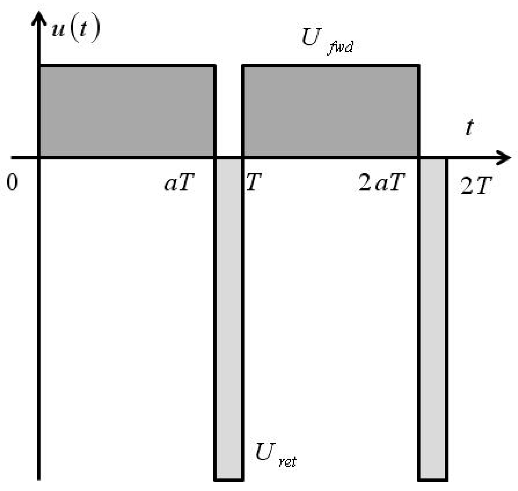
The excitation of both wall interfaces is assumed to be in-phase (symmetric). In general, the period T of wall vibrations is not the same as the one for PG oscillations. The illustration of the square-like wall oscillation waveform used here is shown in Figure 3. The return stroke is very fast and of short duration. The area under forward and return strokes must be equal () to ensure no net (zero-drift) wall motion:
The non-harmonic periodic asymmetric square-waveform function shown in Figure 3 can be expanded in a complex Fourier series with complex coefficients:
Parseval’s identity delivers:
which for a = 0.5 gives a well-known analytical result. Clearly this series will contain both cosine and sine harmonics.
By varying the time-fraction factor “a” which automatically defines the return stroke speed and by using the motion-conservation restriction given with Equation (49), we obtain a variety of square-like waveforms. Due to jump discontinuities in square-like excitations, the Gibbs and “ringing” phenomena arise, and the series cannot possibly converge uniformly and specifically not pointwise at jumps no matter how many Fourier coefficients we employ [51,52,53,54,55,56]. Accordingly, the convergence will be quite slower. The Fourier expansion of the above square function requires at least 100 higher-frequency harmonics to approximate the piecewise continuous function sufficiently well.
4. Results and Discussion
An infinite number of particular solutions can be obtained from the general velocity distribution given by Equation (38). The flow rate and the shear rate can be calculated exactly for the known wall and PG excitations using Equations (40) and (41).
4.1. Unsteady Dynamics and Model Verification
Unsteady laminar flow analytical and numerical computations were coded and compiled in Fortran 95 (standard ISO/IEC 1539-1:1997) high-performance optimizing compiler (Lahey Computer SystemsTM) for rapid calculations. Additionally, slower interactive execution utilizing MATLABTM 7.14 (R2012a, The MathWorksTM) interpreter was used for computations, testing and plotting of results.
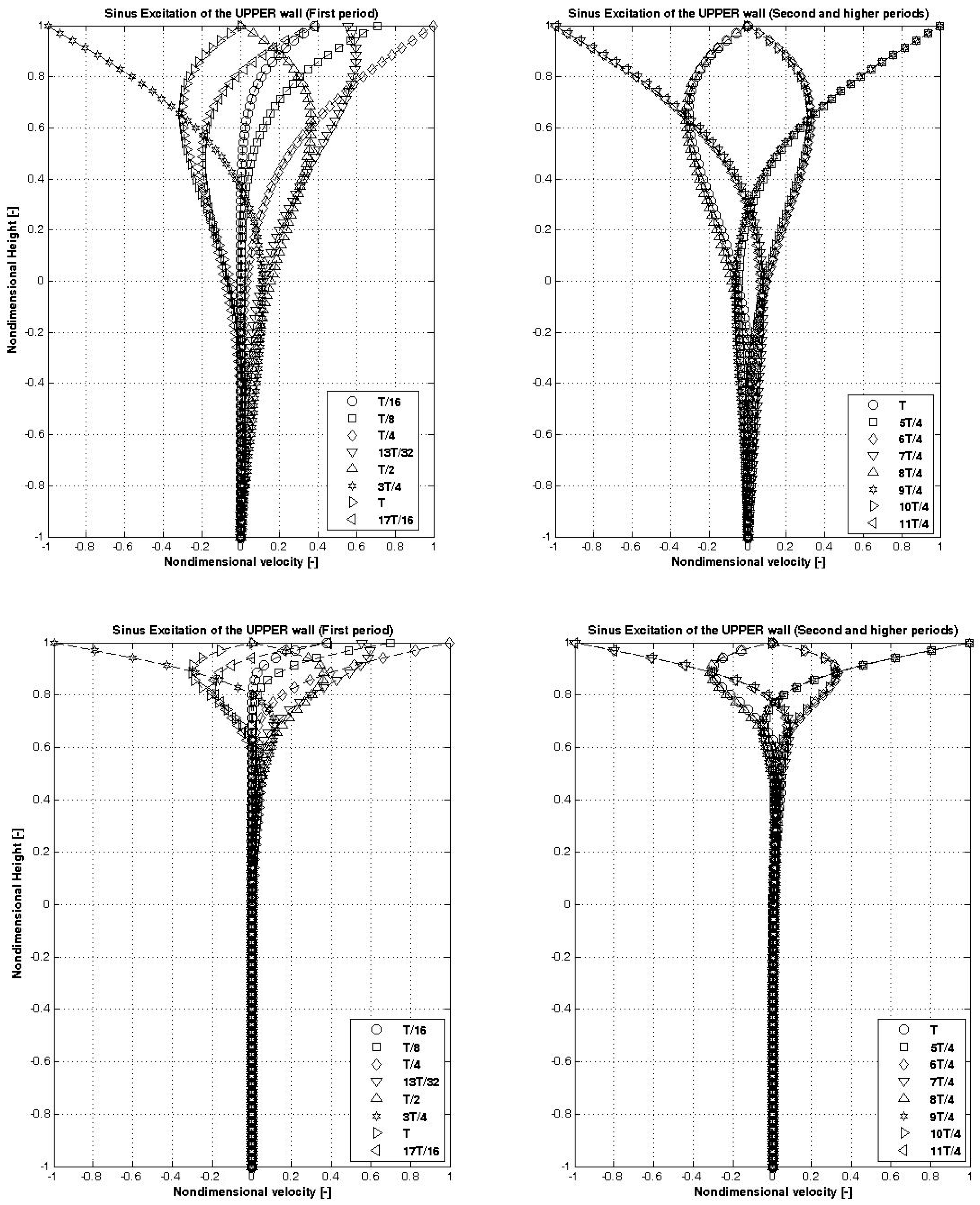
The numerical (FVM-CFD) and analytical results for sinusoidal oscillatory shear-driven Couette–Stokes (CS) flow with an arbitrary phase ψ and unit amplitude in the absence of static and dynamic PGs and for () and, (), are shown in Figure 4. In addition to testing the accuracy of the analytical and the numerical model, many useful conclusions can be made regarding the transient behavior and the effect of the WO number on the penetration depth (zone/radius of influence). The analytical solution and the numerical computations agree within 8+ significant digits throughout the entire spatial-temporal domain.
Lower WO number wall oscillations penetrate deeper into the fluid. For WO numbers less than one, there is essentially no transient behavior, and the flow is basically quasi-steady at all times and faithfully responding to moving boundary with zero phase lag. Transient behavior is best observed in the velocity profiles at T/16 and 17T/16, for both, low and high WO numbers. For higher WO numbers, the transient effects are also apparent in the 2nd and 3rd period. For WO = 10 flow, the lower ¾ of fluid domain is basically unaffected by the upper-wall oscillations. In the case of lower WO = 3.26, only the lower ¼ of fluid depth is unaffected by the upper boundary. The analytical result utilizing the shifting function for dimensionless velocity of harmonically oscillating (upper plate) flow in the absence of PGs yields:
In subsequent computations, analytical and computational efforts were only compared in VFR results. This is to avoid busy graphs. The agreement between the theory and the numerical experiment is always perfect. We have successfully performed transient analysis of all basic flows, such as CT, PO, WO, and ST flows which due to the lack of space cannot be shown here. However, more complex combined flows will reveal all the unsteady dynamics.
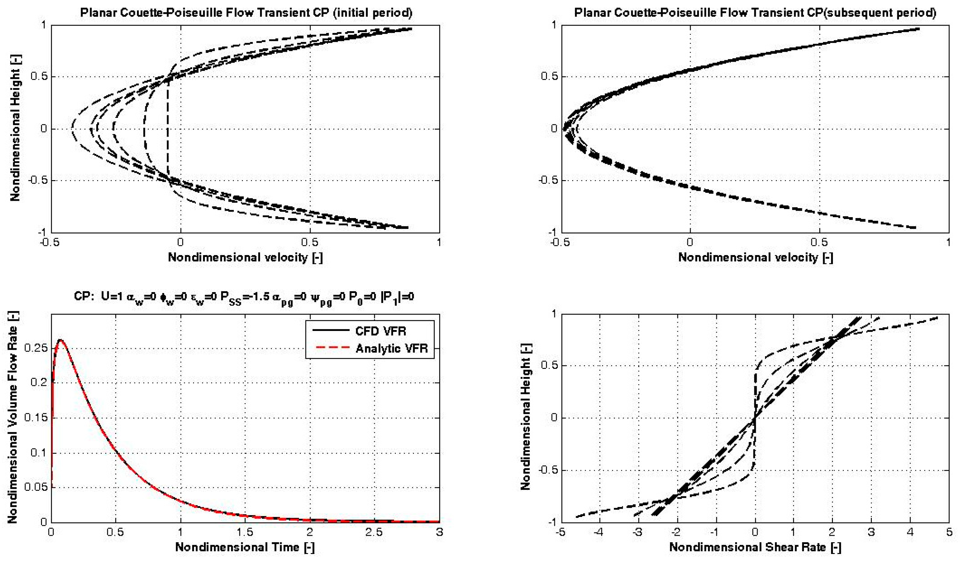
The CP flow transient is shown in Figure 5. This flow incorporates shear and pressure driving. We already know from the analytical CP flow solution that it will result in stalled or zero steady-state VFR. Interestingly, the shear effect overcomes pressure-driven forces initially. One of the reasons is the smaller inertia of a liquid layer in the wall vicinity. The shear rate approaches the steady-state value of rapidly. Since the flow is asymmetric, we cannot use cosine eigenfunctions alone. Using the EEM, which converges everywhere except at the moving boundary (non-compatible BCs), we obtain:
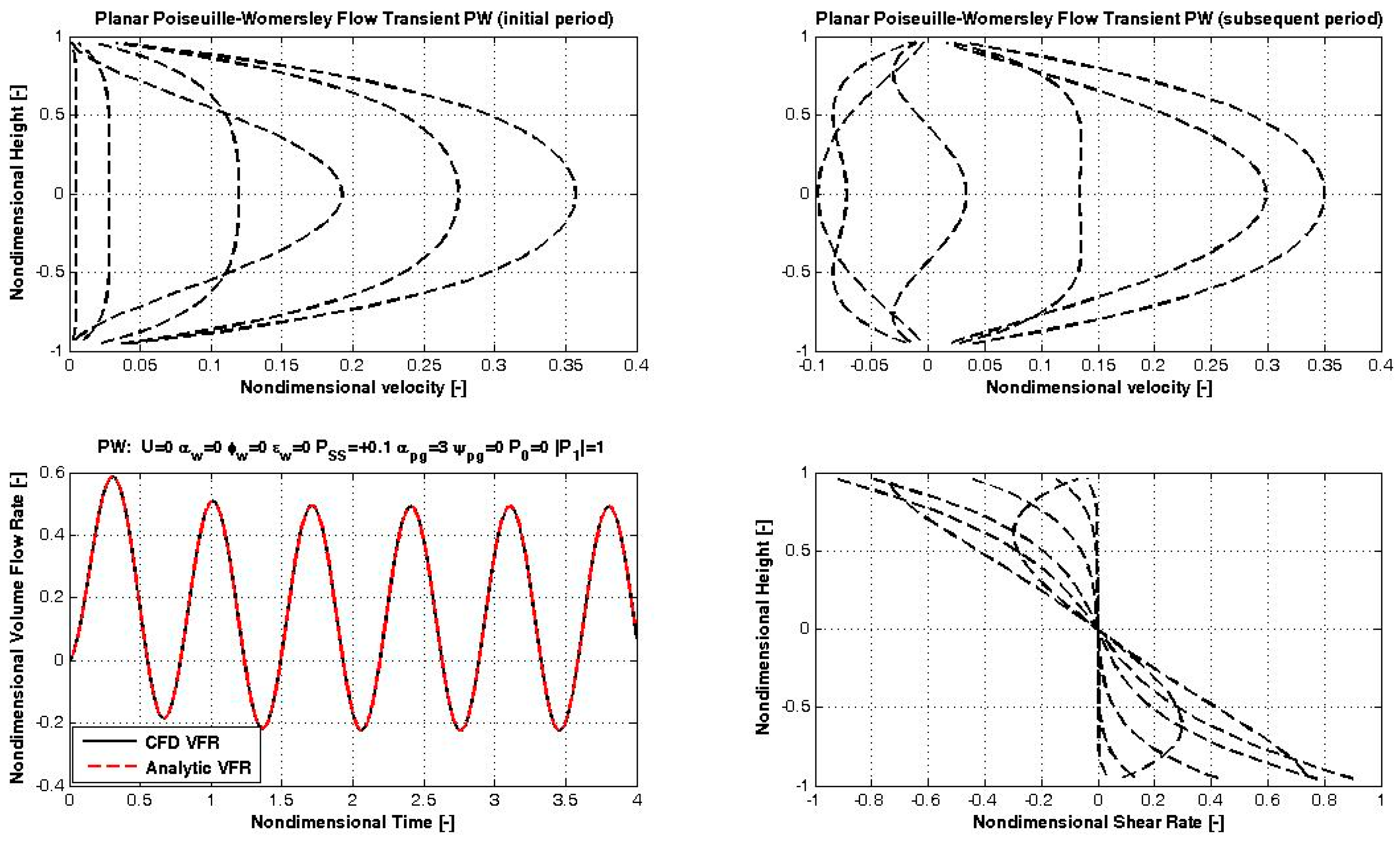
Surprisingly, as it may seem, both series give the same result except at the boundary and the EEM does not converge uniformly. However, it is more general. The unsteady pressure-driven PW flow transient is shown in Figure 6. The pumping action comes from the PG DC-component (0.05) resulting in pulsatile and positive net flow. Flow reversals are similar to pulsatile flow in arterial vessels caused by reciprocating heart pumping. Oscillating shear stresses are essential information in hemodynamic analysis. The classical solution of this problem in terms of elementary functions is given in [4,5,13,14,15], but the solution derived here using Fourier series expansion is perhaps more elegant and more general.
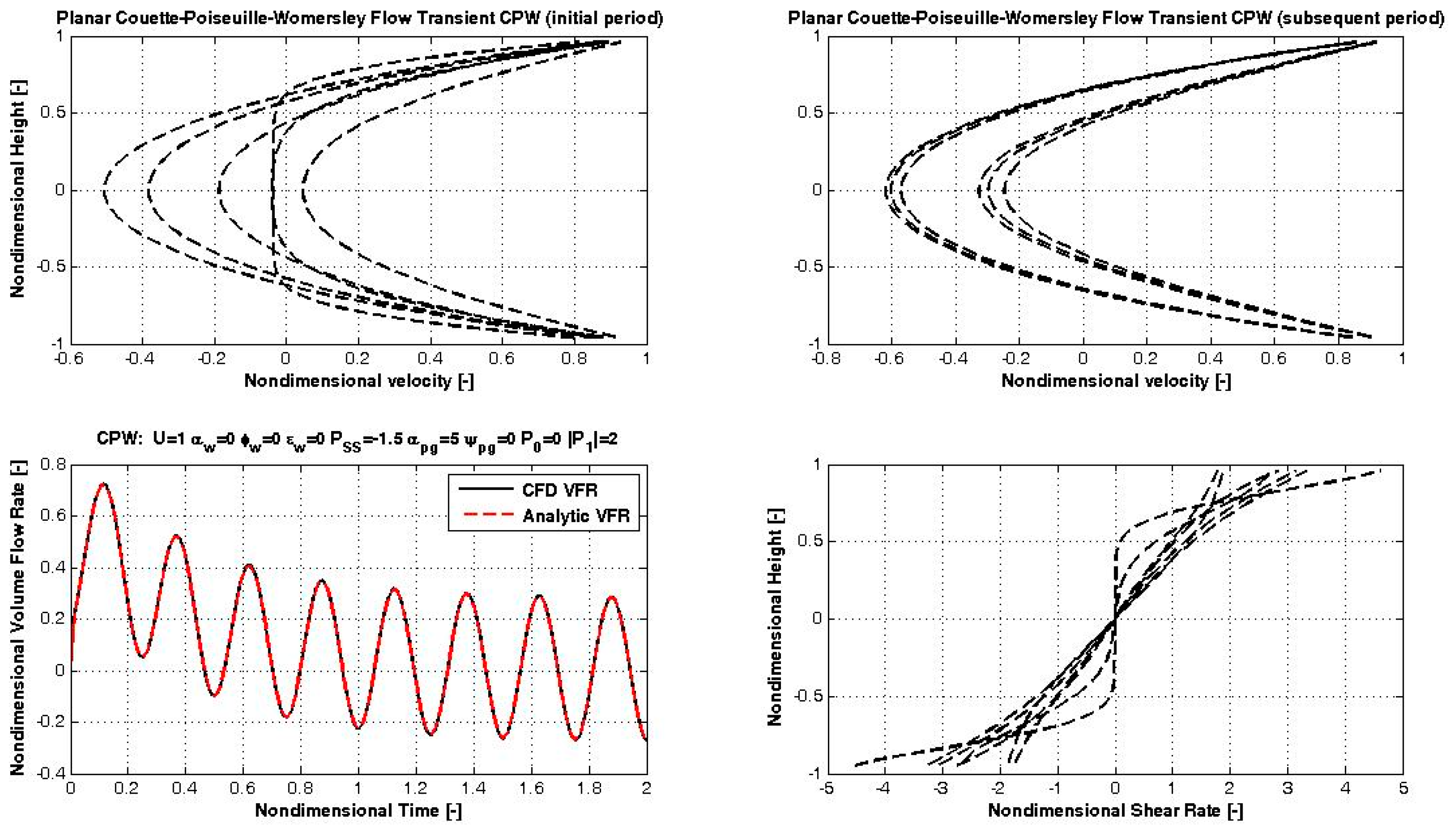
Next, test results treat full transient and QSS solution involving symmetric (ST2) harmonic wall excitations with uniform (CT) components as well as harmonic (WO) PG superimposed onto the steady-state (PO) PG. The analytic solution originates directly from the general solution for the simple wall sinusoidal oscillations. The CPW flow transient is shown in Figure 7. The agreement with CFD is complete. The Womersley component communicates oscillatory fluid behavior.
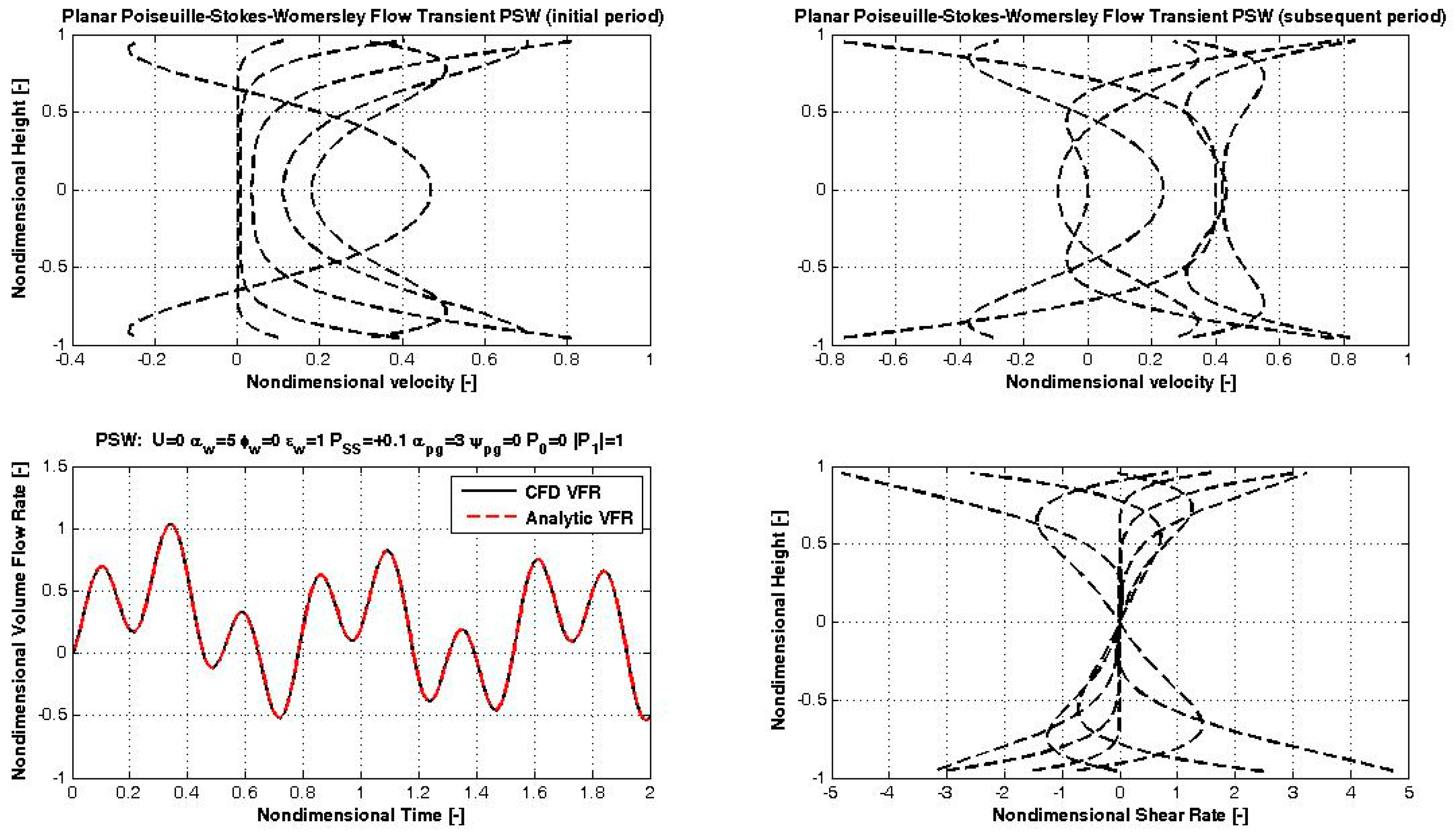
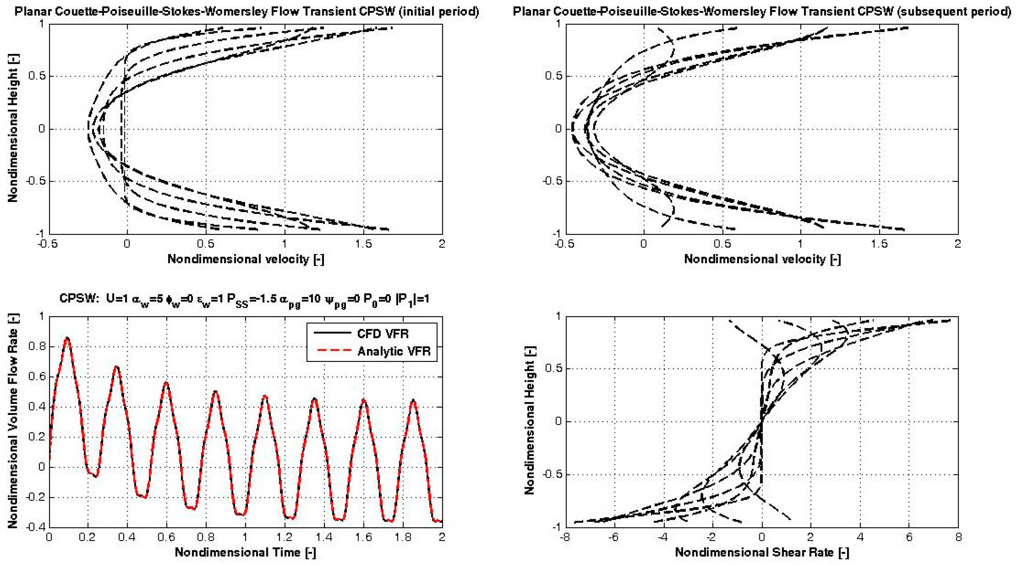
Oscillatory PSW flow is shown in Figure 8. The interaction of the wall and the PG oscillations results in periodic yet non-harmonic flow. The last verification and testing result is reserved for the most complicated harmonic flow so far, i.e., CPSW flow transient and is shown in Figure 9. Again, no net flow exists as we just added simple harmonic (sinusoidal with phase) ST and WO components to steady CP flow. However, the transient and the QSS flow do not look trivial.
Numerical and analytical computations run under different clocks. While we can choose any future time with the analytical solution, the stability- and accuracy-limited numerical solution has to drudgingly march toward it. Since numerical and analytical computations work under different “clocks”, it was sometimes difficult to synchronize discrete times resulting in small discrepancies. However, we already demonstrated excellent agreement between the numerical experiments and theoretical computations involving generalized Fourier series. Many tens of hours were spent investigating various transient and quasi-steady-state oscillatory flows caused by diverse wall and PG dynamics. An article ten-fold in size would be required to show all relevant tests and comparisons between the analytical and numerical results. It suffices to say that all tests and computations were successful and revealed rich and interesting flow patterns even for such linear flows of Newtonian fluid.
4.2. Results for Unsteady Flows with Nonharmonic Wall Oscillation
In the final set of analytical-only results, we present planar non-harmonic shear driving of Newtonian fluids in the presence of steady and dynamic PGs. Rectified-sine function was used to model PGs (Equation (47)), while the non-harmonic wall oscillations were modeled using square-waveform given by Equation (50). Various alternative harmonic and non-harmonic waveforms could be used, which is left only to our imagination. The Fourier series approach works very well, sometimes even with the most bizarre of functions. Numerical solutions always fully agreed with the analytical results.
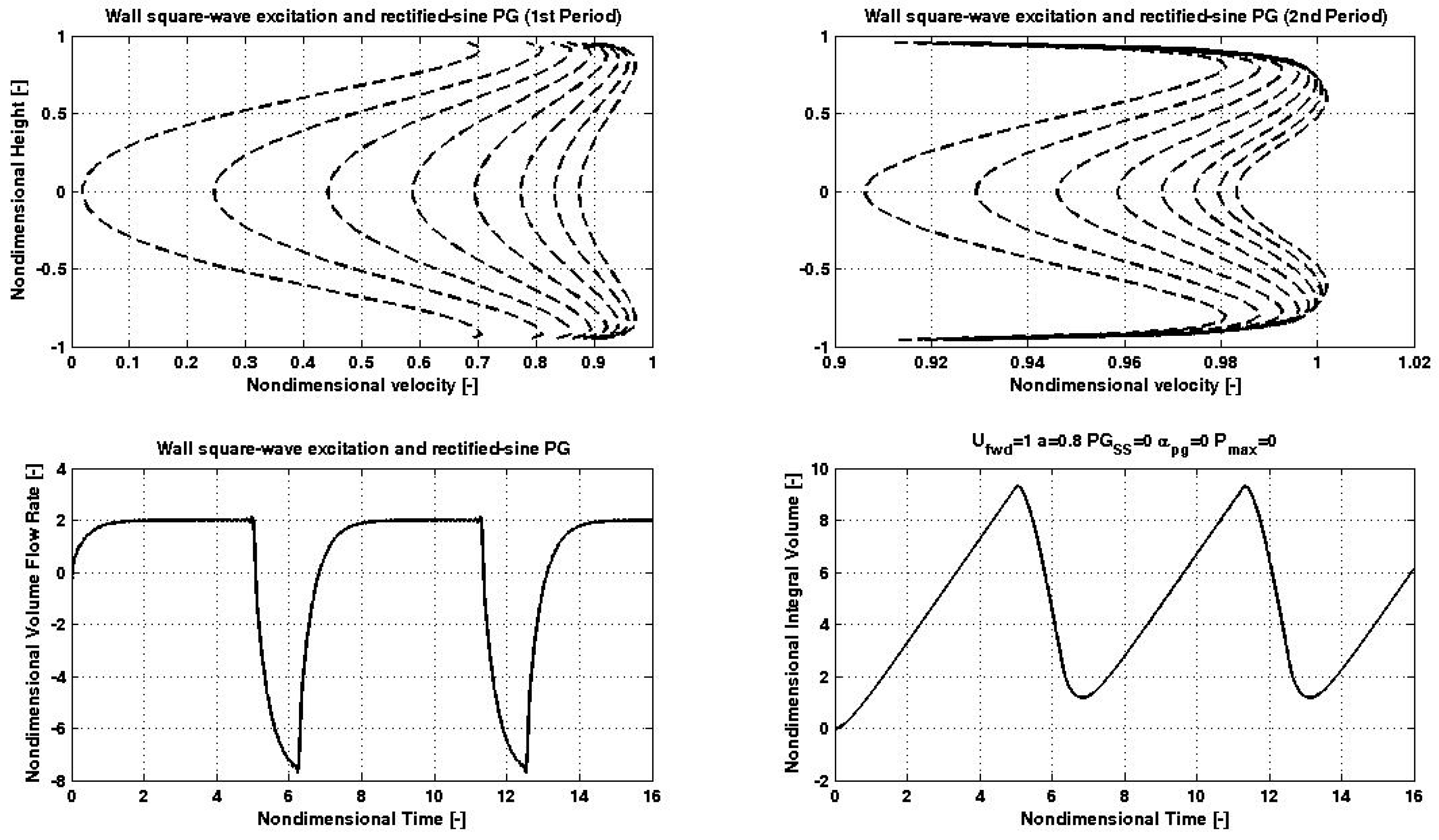
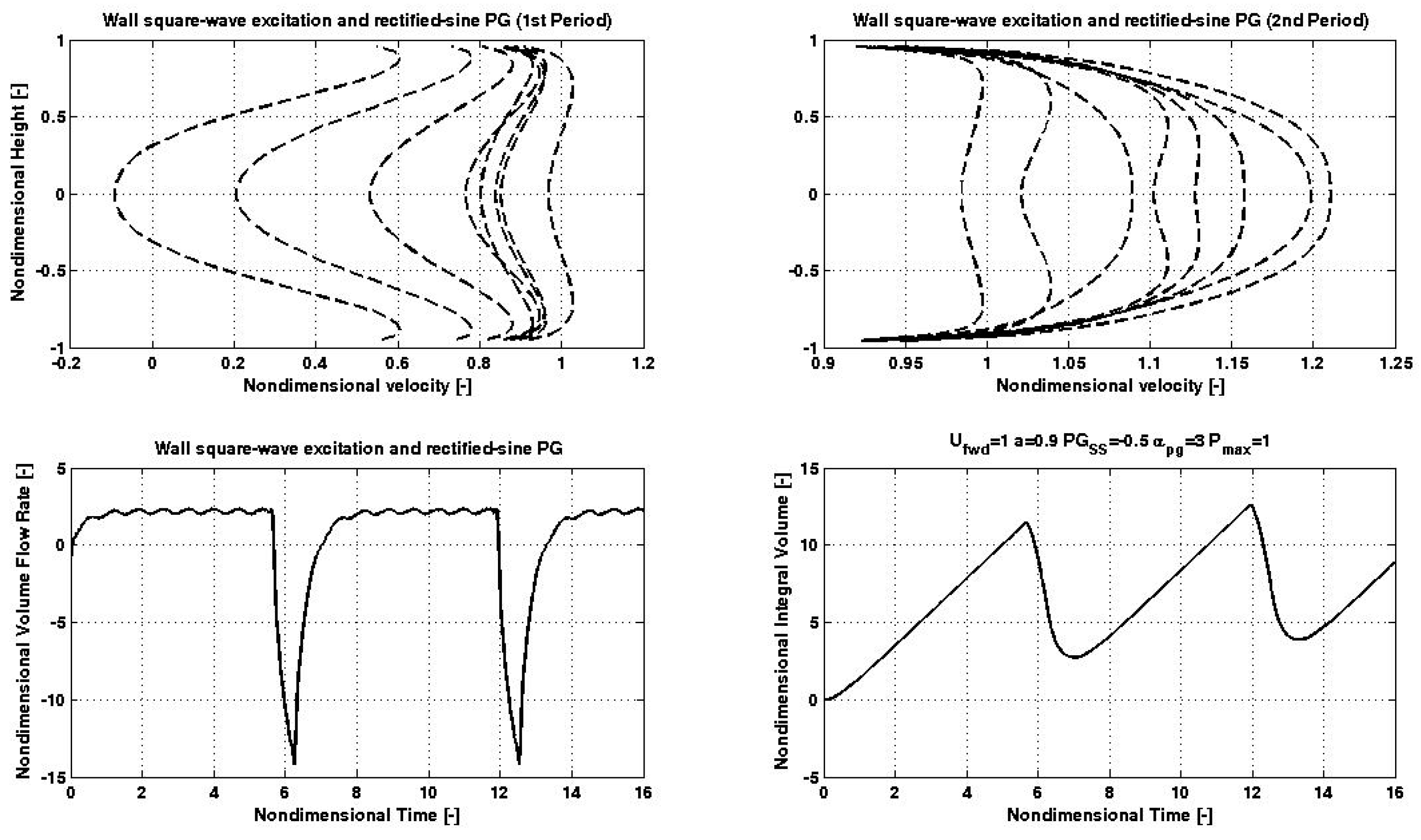
A result for symmetric square-waveform shear-driven flow in the absence of any PGs and period of 2π is shown in Figure 10. The fluid responds to wall-dynamics switching logic between forward and return stroke with inertia and resistance. Integral volume, obtained by analytic integration of Equation (40), shows no net fluid flow other than for small initial transient. Non-harmonic shear-driven planar flow with no PGs is shown in Figure 11. No net flow is obtained with non-harmonic driving except for small initial transient. Finally, the non-harmonic shear-driven flow is being exposed to adverse steady-state PG and proverse rectified-sine dynamic PG with finite Womersley number (WO = 3) is shown in Figure 12. The DC-component of proverse pulsatile PG is able to overcome the adverse negative PO pressure component resulting in positive and somewhat interesting oscillating flow patterns. All numerical experiments were in perfect agreement with the analytical model.
Even though Stokes’ penetration layer decreased significantly for the high WO flows, non-harmonic excitation did not result in net flow rates. However, this is chiefly because of the assumed flow idealizations. No energy equation was solved, and the fluid is linear. Since all the external energies applied in the forward and the return strokes go completely into fluid motion, we could not have expected differently. However, high shear rates in the rapid wall return strokes will result in quadratically higher local dissipation and heating of the liquid, which in turn will lower its viscosity, provided that the heat is being conducted away before the forward strokes. Non-Newtonian fluids (such as blood) are especially well suited for non-harmonic shear driving as their dynamic viscosity changes significantly with the shear rate (increasing or decreasing). Special surface roughness (micro-geometry) and/or coatings may be used to increase shear stress in the forward stroke while decreasing it in the reverse stroke. Last, but not least, rapid return stroke may result in partial or full (molecular and/or apparent) wall slip. Work is in progress to solve similar problem in rigid cylindrical geometry by utilizing Newtonian and various non-Newtonian fluids with or without slip which will be reported in subsequent publications.
Works by Rajagopal et al. [61] and Fetecau and Narahari [62] recently came to our attention. They address IBVP problems somewhat related and similar to ours. Rajagopal et al. [61] investigate unsteady flow with pressure-dependent viscosity and the effect of gravity. The hydromagnetic flow of incompressible viscous fluids between horizontal infinite parallel plates embedded in a porous medium has been analytically studied by Fetecau and Narahari [62]. In particular, the Couette and Stokes problem was considered for known magnetic parameters of fluid and porous medium.
Our future studies will include cylindrical and other geometries with and without boundary slip and various other generalized Newtonian fluid models. Some of these problems will be nonlinear for which some special solution techniques will be applied. Numerically, such problems can be solved with ease, but do not provide general solutions.
5. Conclusions
A unified theory of diffusion-controlled laminar slit flow where the driving force was provided by both variable pressure gradients and wall motion was developed. The eigenfunction expansion method was used to solve the global non-homogeneous linear initial and boundary value problem analytically. Simultaneously, a finite-volume method was used for numerical experiment. The classical results for the steady-state, transient and quasi-steady-state flows were recovered both analytically and numerically with high accuracy and fidelity. Both adverse and proverse pressure gradients were used for fluid pressure driving. Harmonically and non-harmonically oscillating infinite rigid impenetrable flat plates were used for fluid shear driving. We used rectified-sine excitations for pressure gradients in combination with the square-waveform non-harmonic zero-drift wall motion. The effect of wall- and pressure-gradient Womersley numbers on flow dynamics has been studied. No net flow rates could be achieved by non-harmonic oscillations for Newtonian fluid, but that is mostly because several physical effects were neglected, and the energy equation was not coupled in. Ongoing analytical, experimental, and numerical studies will attempt to answer some important questions regarding various microscale flow geometries, partial or full apparent boundary slip condition, change in physical parameters due to local viscous dissipation and heat transfer, shear pumping of non-Newtonian fluids, flow stability, interactions and zone-of-influence from multiple moving surfaces and others.
Funding
This research received no external funding.
Institutional Review Board Statement
Not applicable.
Informed Consent Statement
Not applicable.
Data Availability Statement
Not applicable.
Conflicts of Interest
The author declares no conflict of interest.
Nomenclature
| Symbols | |
| a | Square-waveform time weight parameter, [-] |
| b | Acceleration of the wall boundary, [m/s2] |
| cp | Specific heat capacity at constant pressure, [J/ kg K] |
| f | Natural frequency of oscillation, [Hz] |
| g | Average terrestrial acceleration at sea level, [m/s2] |
| h | Height, [m] |
| k | Thermal conductivity, [W/m K] |
| p | Normal stress—pressure, [Pa] |
| T | Period of oscillations, [s] |
| T | Temperature, [K] |
| t | Time, [s] |
| U | Velocity (maximum wall velocity), [m/s] |
| u,v,w | Velocity in axial (longitudinal) direction, [m/s] |
| Greek Symbols | |
| α | Womersley number, [-] |
| β | Coefficient of thermal expansion, [K−1] |
| δ | Thickness, Stokes’ (diffusion) penetration layer, [m] |
| δij | Kronecker delta (=1 for i = j, otherwise = 0 for i ≠ j), [-] |
| Shear rate, [s−1] | |
| Φ | Dissipation function, [kg m−1·s−3 or W/m3] |
| μ | Dynamic viscosity, [Pa s] |
| ρ | Density, [kg/m3] |
| τ | Shear stress, [Pa] |
| ω | Vorticity, [rad/s] |
| Abbreviations | |
| BC | Boundary condition |
| BVP | Boundary value problem |
| CFD | Computational fluid dynamics |
| C-N | Crank–Nicolson implicit scheme |
| CP | Couette–Poiseuille laminar flow |
| CPSW | Couette–Poiseuille–Stokes–Womersley laminar flow |
| CT | Couette (planar) flow |
| CS | Couette–Stokes flow |
| CTCS | Central Time Central Space |
| EEM | Eigenfunction expansion (method) |
| FD | Finite difference |
| FTCS | Forward Time Central Space |
| FVM | Finite-volume method |
| IC | Initial condition |
| IBVP | Initial boundary value problem |
| MD | Molecular dynamics |
| MMC | Metropolis Monte Carlo |
| N-S | Navier–Stokes hydrodynamic equation |
| ODE | Ordinary differential equation |
| PDE | Partial differential equation |
| PO | Poiseuille (planar) flow |
| PW | Poiseuille–Womersley flow |
| QSS | Quasi-steady-state |
| SOV | Separation of variables |
| ST | Stokes’ flow |
| ST1 | Stokes’ flow (1st problem) |
| ST2 | Stokes’ flow (2nd problem) |
| TDMA | Thomas’ tridiagonal matrix algorithm |
| WO | Womersley laminar flow (also Womersley number) |
References
- Lamb, H. Hydrodynamics, 6th ed.; Dover Publications: New York, NY, USA, 1945. [Google Scholar]
- Schlichting, H. Boundary-Layer Theory, 7th ed.; Mc-Graw Hill: New York, NY, USA, 1987. [Google Scholar]
- Batchelor, G.K. An Introduction to Fluid Dynamics; Cambridge University Press: Cambridge, UK, 2000. [Google Scholar]
- Landau, L.D.; Lifshitz, E.M. Fluid Mechanics, 6th ed.; Butterworth Heinemann: Oxford, UK, 1987. [Google Scholar]
- White, F.M. Viscous Fluid Flow; McGraw-Hill, Inc.: New York, NY, USA, 1991. [Google Scholar]
- Sherman, F.S. Viscous Flow; McGraw-Hill: New York, NY, USA, 1991. [Google Scholar]
- Panton, R.L. Incompressible Flow, 3rd ed.; John Wiley & Sons: Hoboken, NJ, USA, 2005. [Google Scholar]
- Kundu, P.K.; Cohen, I.M. Fluid Mechanics, 4th ed.; Elsevier: New York, NY, USA, 2007. [Google Scholar]
- Wang, C.Y. Exact solutions of the steady-state Navier-Stokes equations. Annu. Rev. Fluid Mech. 1991, 23, 159–177. [Google Scholar] [CrossRef]
- Drazin, P.G.; Reid, W.H. Hydrodynamic Stability; Cambridge University Press: Cambridge, UK, 1981. [Google Scholar]
- Sexl, T.; Über den von, E.G. Richardson entdeckten “Annulareffekt”. Zeit. Phys. 1930, 61, 349–362. [Google Scholar] [CrossRef]
- Womersley, J.R. Method for the calculation of velocity, rate of flow, and viscous drag in arteries when the pressure gradient is known. J. Physiol. 1955, 127, 553–563. [Google Scholar] [CrossRef]
- Berker, R. Intégration des équations du movement d’un fluide visqueux incompressible. In Handbuch der Physik; Flugge, S., Ed.; Springer: Berlin, Germany, 1963; Volume VIII/2, pp. 1–384. [Google Scholar]
- Wang, C.Y. Exact Solutions of the Unsteady Navier-Stokes Equations. Appl. Mech. Rev. 1989, 42, S269–S282. [Google Scholar] [CrossRef]
- Loudon, C.; Tordesillas, A. The Use of the Dimensionless Womersley Number to Characterize the Unsteady Nature of Internal Flow. J. Theor. Biol. 1998, 191, 63–78. [Google Scholar] [CrossRef]
- Nichols, W.N.; O’Rourke, M.F. McDonald’s Blood Flow in Arteries, 3rd ed.; Edward Arnold: London, UK, 1990. [Google Scholar]
- Daidzic, N.E. Application of Womersley Model to Reconstruct Pulsatile Arterial Hemodynamics based on Doppler Ultrasound Measurements. J. Fluids Eng. 2014, 136, 041102. [Google Scholar] [CrossRef]
- Daidzic, N.E.; Hossain, M.S. The Model of Micro-Fluidic Pump with Vibrating Boundaries. In Proceedings of the 14th International Conference on Applied Mechanics and Mechanical Engineering, Cairo, Egypt, 25–27 May 2010. [Google Scholar]
- Hossain, S.; Daidzic, N.E. The Shear-Driven Fluid Motion Using Oscillating Boundaries. J. Fluids Eng. 2012, 134, 051203. [Google Scholar] [CrossRef]
- Carslaw, H.S.; Jaeger, J.C. Conduction of Heat in Solids, 2nd ed.; Clarendon Press: Oxford, UK, 1959. [Google Scholar]
- He, X.; Luo, L.-S. Lattice Boltzmann Model for the Incompressible Navier-Stokes Equation. J. Stat. Phys. 1997, 88, 927–944. [Google Scholar] [CrossRef]
- Chen, S.; Doolen, G.D. Lattice Boltzmann Method for Fluid Flows. Annu. Rev. Fluid Mech. 1998, 30, 329–364. [Google Scholar] [CrossRef] [Green Version]
- Cercignani, C. Ludwig Boltzman: The Man Who Trusted Atoms; Oxford University Press, Inc.: New York, NY, USA, 1998. [Google Scholar]
- Succi, S. The Lattice Boltzmann Equation: For Fluid Dynamics and Beyond; Oxford University Press, Inc.: New York, NY, USA, 2001. [Google Scholar]
- Allen, M.P.; Tildesley, D.J. Computer Simulation of Liquids; Oxford Science Publications, Inc.: New York, NY, USA, 1987. [Google Scholar]
- Koplik, J.; Banavar, J.R.; Willemsen, J.F. Molecular dynamics of fluid flow at solid surfaces. Phys. Fluids A Fluid Dyn. 1989, 1, 781–794. [Google Scholar] [CrossRef]
- Koplik, J.; Banavar, J.R. Continuum Deductions from Molecular Hydrodynamics. Annu. Rev. Fluid Mech. 1995, 27, 257–292. [Google Scholar] [CrossRef]
- Thompson, P.A.; Troian, S.M. A general boundary condition for liquid flow at solid surfaces. Nature 1997, 389, 360–362. [Google Scholar] [CrossRef]
- Leach, A.R. Molecular Modeling: Principles and Applications, 2nd ed.; Pearson: Harlow, UK, 2001. [Google Scholar]
- Karniadakis, G.; Beskok, A.; Aluru, N. Microflows and Nanoflows: Fundamentals and Simulation; Springer: Berlin, Germany, 2005. [Google Scholar]
- Nguyen, N.-T.; Wereley, S.T. Fundamentals and Applications of Microfluidics; Artech House: Boston, MA, USA, 2006. [Google Scholar]
- McDonald, D.A. The relation of pulsatile pressure to flow in arteries. J. Physiol. 1955, 127, 533–552. [Google Scholar] [CrossRef] [PubMed]
- Hale, J.F.; McDonald, D.A.; Womersley, J.R. Velocity profiles of oscillating arterial flow, with some calculations of viscous drag and the Reynolds number. J. Physiol. 1955, 128, 629–640. [Google Scholar] [CrossRef] [PubMed]
- Womersley, J. XXIV. Oscillatory motion of a viscous liquid in a thin-walled elastic tube—I: The linear approximation for long waves. Lond. Edinb. Dublin Philos. Mag. J. Sci. 1955, 46, 199–221. [Google Scholar] [CrossRef]
- Womersley, J.R. Oscillatory Flow in Arteries: The Constrained Elastic Tube as a Model of Arterial Flow and Pulse Transmission. Phys. Med. Biol. 1957, 2, 178–187. [Google Scholar] [CrossRef]
- Ku, D.N. Blood Flow in Arteries. Annu. Rev. Fluid Mech. 1997, 29, 399–434. [Google Scholar] [CrossRef]
- Giusti, A.; Mainardi, F. A dynamic viscoelastic analogy for fluid-filled elastic tubes. Meccanica 2016, 51, 2321–2330. [Google Scholar] [CrossRef] [Green Version]
- Cinthio, M.; Ahlgren, Å.R.; Bergkvist, J.; Jansson, T.; Persson, H.W.; Lindström, K. Longitudinal movements and resulting shear strain of the arterial wall. Am. J. Physiol.-Heart Circ. Physiol. 2006, 291, H394–H402. [Google Scholar] [CrossRef] [Green Version]
- Tikhonov, A.N.; Samarskii, A.A. Equations of Mathematical Physics; Dover Publications, Inc.: New York, NY, USA, 1990. [Google Scholar]
- Strauss, W.A. Partial Differential Equations: An Introduction; John Wiley & Sons, Inc.: New York, NY, USA, 1992. [Google Scholar]
- Tolstov, G.P. Fourier Series; Dover Publications, Inc.: New York, NY, USA, 1976. [Google Scholar]
- Cooper, J. Introduction to Partial Differential Equations with MATLAB; Birkhäuser: Boston, MA, USA, 1998. [Google Scholar]
- Haberman, R. Applied Partial Differential Equations: With Fourier Series and Boundary Value Problems, 4th ed.; Pearson Prentice Hall: Upper Saddle River, NJ, USA, 2004. [Google Scholar]
- Riesz, F.; Sz-Nagy, B. Functional Analysis; Frederick Ungar Publishing Co., Inc.: New York, NY, USA, 1972. [Google Scholar]
- Kreyszig, E. Introductory Functional Analysis with Applications, 4th ed.; John Wiley & Sons: New York, NY, USA, 1978. [Google Scholar]
- Curtain, R.F.; Pritchard, A.J. Functional Analysis in Modern Applied Mathematics; Academic Press: London, UK, 1977. [Google Scholar]
- Kolmogorov, A.N.; Fomin, S.V. Introductory Real Analysis; Dover Publications, Inc.: New York, NY, USA, 1970. [Google Scholar]
- MacCluer, C.R. Boundary Value Problems and Orthogonal Expansions; IEEE Press: New York, NY, USA, 1994. [Google Scholar]
- Burk, F. Lebesgue Measure and Integration; John Wiley & Sons: New York, NY, USA, 1998. [Google Scholar]
- Shilov, G.E.; Gurevich, B.L. Integral, Measure, and Derivative: A Unified Approach; Dover Publications, Inc.: New York, NY, USA, 1977. [Google Scholar]
- Boyce, W.E.; DiPrima, R.C. Elementary Differential Equations and Boundary Value Problems, 9th ed.; John Wiley & Sons, Inc.: Hoboken, NJ, USA, 2010. [Google Scholar]
- Carslaw, H.S. An Introduction to the Theory of Fourier’s Series and Integrals, 3rd ed.; Dover Publications, Inc.: New York, NY, USA, 1950. [Google Scholar]
- Churchill, R.V.; Brown, J.W. Fourier Series and Boundary Value Problems, 3rd ed.; McGraw-Hill: New York, NY, USA, 1985. [Google Scholar]
- Kreyszig, E. Advanced Engineering Mathematics, 4th ed.; John Wiley & Sons: New York, NY, USA, 1979. [Google Scholar]
- Smith, L.P. Mathematical Methods for Scientists and Engineers; Prentice Hall, Inc.: New York, NY, USA, 1953. [Google Scholar]
- Tang, K.T. Mathematical Methods for Engineers and Scientists; Springer: Berlin, Germany, 2007. [Google Scholar]
- Patankar, S.V. Numerical Heat Transfer and Fluid Flow; Hemisphere Publishing Corporation, McGraw-Hill Book Company: Washington, DC, USA, 1980. [Google Scholar]
- Press, W.H.; Teukolsky, S.A.; Vetterling, W.T.; Flannery, B.P. Numerical Recipes in FORTRAN: The Art of Scientific Computing, 2nd ed.; Cambridge University Press: Cambridge, UK, 1992. [Google Scholar]
- Thomas, J.W. Numerical Partial Differential Equations: Finite Difference Methods; Springer Science and Business Media LLC: New York, NY, USA, 1995. [Google Scholar]
- Ferziger, J.H.; Peric, M. Computational Methods for Fluid Dynamics; Springer: Berlin, Germany, 1997. [Google Scholar]
- Rajagopal, K.; Saccomandi, G.; Vergori, L. Unsteady flows of fluids with pressure dependent viscosity. J. Math. Anal. Appl. 2013, 404, 362–372. [Google Scholar] [CrossRef]
- Fetecau, C.; Narahari, M. General Solutions for Hydromagnetic Flow of Viscous Fluids between Horizontal Parallel Plates through Porous Medium. J. Eng. Mech. 2020, 146, 04020053. [Google Scholar] [CrossRef]
Figure 1.
General inclined planar flow geometry with two oscillating boundaries. Not to scale.

Figure 2.
Rectified-sine function describing periodic PG dynamics. Not to scale.

Figure 3.
Square-like excitations with respective rapid return stroke describing periodic non-harmonic wall motion. The surface areas in forward and return stroke must be equal. Not to scale.
Figure 3.
Square-like excitations with respective rapid return stroke describing periodic non-harmonic wall motion. The surface areas in forward and return stroke must be equal. Not to scale.

Figure 4.
Upper plate sinusoidal oscillatory Couette-Stokes flow for (upper) and (lower) graph for the first (LHS) and 2nd and 3rd periods (RHS) are shown. (Analytic—dashed lines; CFD—markers/symbols).
Figure 4.
Upper plate sinusoidal oscillatory Couette-Stokes flow for (upper) and (lower) graph for the first (LHS) and 2nd and 3rd periods (RHS) are shown. (Analytic—dashed lines; CFD—markers/symbols).

Figure 5.
Starting Transients for the planar CP flow.

Figure 6.
Starting transient for the pulsatile PW rigid-slit flow.

Figure 7.
Starting transient for the pulsatile CPW flow.

Figure 8.
Starting transient for the simple harmonic PSW flow.

Figure 9.
Starting transient for the simple harmonic CPSW flow.

Figure 10.
Dynamics of non-harmonic shear-driven slit flow (a = 0.5).

Figure 11.
Dynamics of non-harmonic shear-driven slit flow (a = 0.8).

Figure 12.
Dynamics of non-harmonic shear-driven flow (a = 0.9) with external PGs.

Publisher’s Note: MDPI stays neutral with regard to jurisdictional claims in published maps and institutional affiliations. |
© 2022 by the author. Licensee MDPI, Basel, Switzerland. This article is an open access article distributed under the terms and conditions of the Creative Commons Attribution (CC BY) license (https://creativecommons.org/licenses/by/4.0/).
Share and Cite
MDPI and ACS Style
Daidzic, N.E. Unified Theory of Unsteady Planar Laminar Flow in the Presence of Arbitrary Pressure Gradients and Boundary Movement. Symmetry 2022, 14, 757. https://0-doi-org.brum.beds.ac.uk/10.3390/sym14040757
AMA Style
Daidzic NE. Unified Theory of Unsteady Planar Laminar Flow in the Presence of Arbitrary Pressure Gradients and Boundary Movement. Symmetry. 2022; 14(4):757. https://0-doi-org.brum.beds.ac.uk/10.3390/sym14040757
Chicago/Turabian StyleDaidzic, Nihad E. 2022. "Unified Theory of Unsteady Planar Laminar Flow in the Presence of Arbitrary Pressure Gradients and Boundary Movement" Symmetry 14, no. 4: 757. https://0-doi-org.brum.beds.ac.uk/10.3390/sym14040757
Note that from the first issue of 2016, this journal uses article numbers instead of page numbers. See further details here.