Identifying Appropriate Locations for the Accelerated Weathering of Limestone to Reduce CO₂ Emissions

Abstract

The reduction in CO₂ emissions is a major task for the coming decades. Accelerated weathering of limestone (AWL) can be used to capture CO₂ from effluent gas streams and store it as bicarbonate in marine environments. We give an overview of the fundamental aspects of AWL, including associated CO₂ emissions during the operation of AWL, characteristics of the accumulating bicarbonate-rich product water, and factors influencing the outgassing of CO₂ from the ocean back into the atmosphere. Based on these aspects, we identify locations where AWL could be carried out favorably. The energy demand for AWL reduces the theoretical CO₂ sequestration potential, for example, by only 5% in the case of a 100 km transport of limestone on roads. AWL-derived product water is characterized by high alkalinity but low pH values and, once in contact with the atmosphere, passive outgassing of CO₂ from AWL-derived water occurs. This process is mainly driven by the difference between the fCO₂ in the atmosphere and the oceanic surface layer, as well as the sea surface temperature at the discharge site. Promising sites for AWL may be in Florida or around the Mediterranean Sea, where outgassing could be prevented by injections into deep water layers.

1. Introduction

Despite knowing about the severe consequences of climate change on our planet, the concentration of CO₂ is still rising by 2–3 ppmv every year [1]. If an increase in the global average temperature is to be kept well below 2 °C, in comparison to pre-industrial levels as intended by the Paris Agreement [2], a 40% to 70% reduction in greenhouse gas emissions is needed until 2050 [3]. Reductions of this magnitude may only be achieved via a combination of different technologies, including geoengineering approaches such as AWL.

In nature, CO₂ is removed from the atmosphere via the weathering of carbonate and silicate rocks on a 10,000- to 100,000-year timescale (e.g., [4,5]). For AWL, the process of carbonate rock weathering is mimicked by reacting a CO₂–rich effluent gas with a limestone suspension in a reactor. The net reaction being:

$${\mathrm{CO}}_2+{\mathrm{CaCO}}_3+{\mathrm{H}}_2\mathrm{O}\leftrightarrow {\mathrm{Ca}}^{2+}+{2\mathrm{HCO}}_3^{-}$$

(1)

As the partial pressure of CO₂ is significantly elevated in the reactor, the dissolution of calcium carbonate is carried out within minutes instead of thousands of years. The resulting bicarbonate-rich product water is characterized by a high total alkalinity (TA) and might be used to counteract ocean acidification if disposed of into a marine environment.

Although the concept of AWL is not new [6], it has only been performed in lab-scale or mid-scale applications for research purposes [7,8,9,10,11]. It has been shown that up to 97% of the CO₂ could be captured from a gas stream in a laboratory [9]. However, a mid-scale application suitable to scrub, e.g., small, combined heat and power plants with an electric power generation of 60 kW, was able to remove up to 55% of the CO₂ [11].

Using ocean models, it has been shown that AWL is more effective in storing CO₂ and weakening ocean acidification impacts in comparison to a direct CO₂ injection [10,12]. A recent study pointed out that very shallow shelf seas might not be suitable for AWL, as the probability of CO₂ outgassing and reprecipitation of calcium carbonate is high [13]. The identification of favorable discharge sites for large-dimensioned applications is still missing.

To identify such locations, we firstly give an overview of relevant aspects concerning the application of AWL and the properties of AWL-derived water. Secondly, we perform a sensitivity study to evaluate potential outgassing of CO₂ from AWL-derived water back into the atmosphere. These parts contain basic but fundamental aspects concerning AWL. However, discussions with other scientists revealed that these aspects are often not understood, and an overview is missing in the literature. Based on the information gained in the first two parts, we finally identify areas where AWL could be performed favorably, and which should be evaluated in more detail in upcoming studies.

2. Theoretical Assessment of AWL to Reduce CO₂ Emissions

According to Equation (1), each ton of limestone can sequester approximately 440 kgCO₂, depending on the purity of the rock material and the initial chemistry of the carbonate system of the utilized water. This sequestration potential is relatively low in comparison to other minerals, e.g., one ton of forsterite (Mg₂SiO₄) can sequester approximately 1250 kgCO₂ [14]. However, the dissolution rates of both minerals likewise differ with the calcium carbonate (calcite) dissolution rate being four orders of magnitude higher than that of forsterite [15,16]. Because of the high dissolution rate of calcium carbonate and because it covers approximately 10% of the land surface [17], we focus on limestone as the rock source for AWL. If the total amount of limestone would be equally distributed, approximately 38,000 Gt would be within 10 km of the coast [18], sufficient to store up to 16,720 GtCO₂. Thus, a significant amount of the 34.4 GtCO₂·yr⁻¹ that was emitted from fossil fuel combustion and other industrial processes from 2008 to 2017 [19] could be sequestered during the next decade, or even longer. Quarrying limestone generates considerable amounts of fine limestone powder that cannot be used for typical industrial processes, and must be disposed of, leading to environmental problems [20]. Because of its high surface area, this powder might prove to be ideal for use in AWL.

As the theoretical sequestration potential is reduced by limestone processing, transport, and AWL itself, a critical examination of every step is necessary for a full evaluation of AWL. The energy demand and CO₂ emissions during major process steps are given in

Table 1. Energy demand and CO₂ emissions of the major process steps during the application of AWL. Negative values represent CO₂ uptake.

Process	Energy Demand in MJ·t−1	Emission of CO2 or CO2eq in kg·t−1
Extraction processes and comminution 1	108 a	15 a
Transport method (data per km)
Road	1.3 b	0.062 c
Rail freight	0.2 b	0.022 c
Inland waterways	0.2 b	0.031c
Pumping for AWL 2	5	1.14
Theoretical CO2 sequestration		−440
Net CO2 sequestration (100 km transport on road)		−418

¹ grinding to ~100 µm; ²: see Supporting Information for details on the calculation ^a [18]; ^b [21]; ^c [22].

. The values of these two parameters are fixed for limestone mining and processing, whereas the net CO₂ sequestration potential depends on the distance over which the limestone must be transported. Every 100 km transport on roads decreases the sequestration potential by roughly 1.5%. The complete process, including 100 km transport on roads, reduces the maximum possible sequestration from 440 kgCO₂ per ton limestone to a net sequestration of 418 kgCO₂ per ton limestone: a reduction of only 5%.

The effects of AWL on marine carbonate chemistry are often equalized with other ocean alkalinization techniques that are under consideration for carbon sequestration. Several advantages and disadvantages of the single techniques are summarized by Renforth and Henderson [21]. All alkalinization techniques enhance the oceanic TA. Dissolution of quicklime (CaO) or slaked lime (Ca(OH)₂), for example, leads to the formation of OH⁻ ions, and is followed by a strong increase in pH. In contrast, AWL-derived water is characterized by a pH value of approximately 6.5 due to the high pCO₂ (~150,000 ppmv) within the reactor [12]. Once back in contact with the atmosphere, the dissolved CO₂ outgasses until equilibrium with the atmosphere is reached. Due to the outgassing, the final pH of the solution increases to values above the initial seawater pH.

Using the Finite-Volume, 3D primitive-equation Community Ocean Model (FVCOM; [23]) to calculate hydrodynamic conditions, coupled with a module to model the ocean carbonate system (mocsy; [24]), we modelled differences in pH, after applying AWL at a 750 MW coal-fired power plant close to Wilhelmshaven (Germany). We assumed a treatment of the complete flue gas of the power plant and simulated the discharge of the resulting bicarbonate-rich product water into the adjacent North Sea. Water that is discharged directly after it exits the reactor decreases the pH_T (pH_T: pH on the total scale) of up to 1 pH_T unit at the coastal area around the discharge site (Figure 1b). If the water is actively degassed to equilibrium of CO₂ with the atmosphere before it is discharged, the pH_T increases (Figure 1c), while the alkalinity is not changing. Note that in practice, complete degassing is associated with precipitation of calcium carbonate, which in turn liberates CO₂ that has previously been sequestered during AWL. Precipitation of calcium carbonate can be prevented by diluting AWL-derived water with seawater [12]. For more information on the model setup, see the Supporting Information and [13]. Thus, depending on the final technical realization, the properties of AWL-derived water can be different. Without degassing, the efficiency of AWL in terms of CO₂ sequestration is significantly higher, but a discharge is accompanied by decreasing pH. In contrast, degassing reduces AWL efficiency, but as the water is characterized by high TA and high pH, discharge could be beneficial for marine ecosystems against progressing ocean acidification.

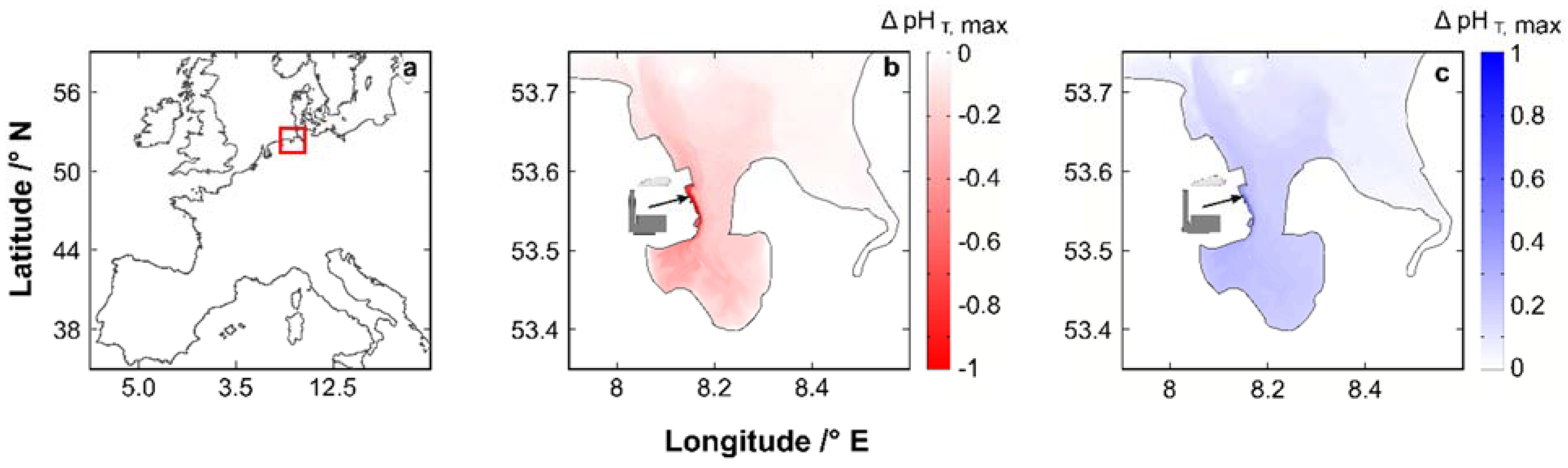
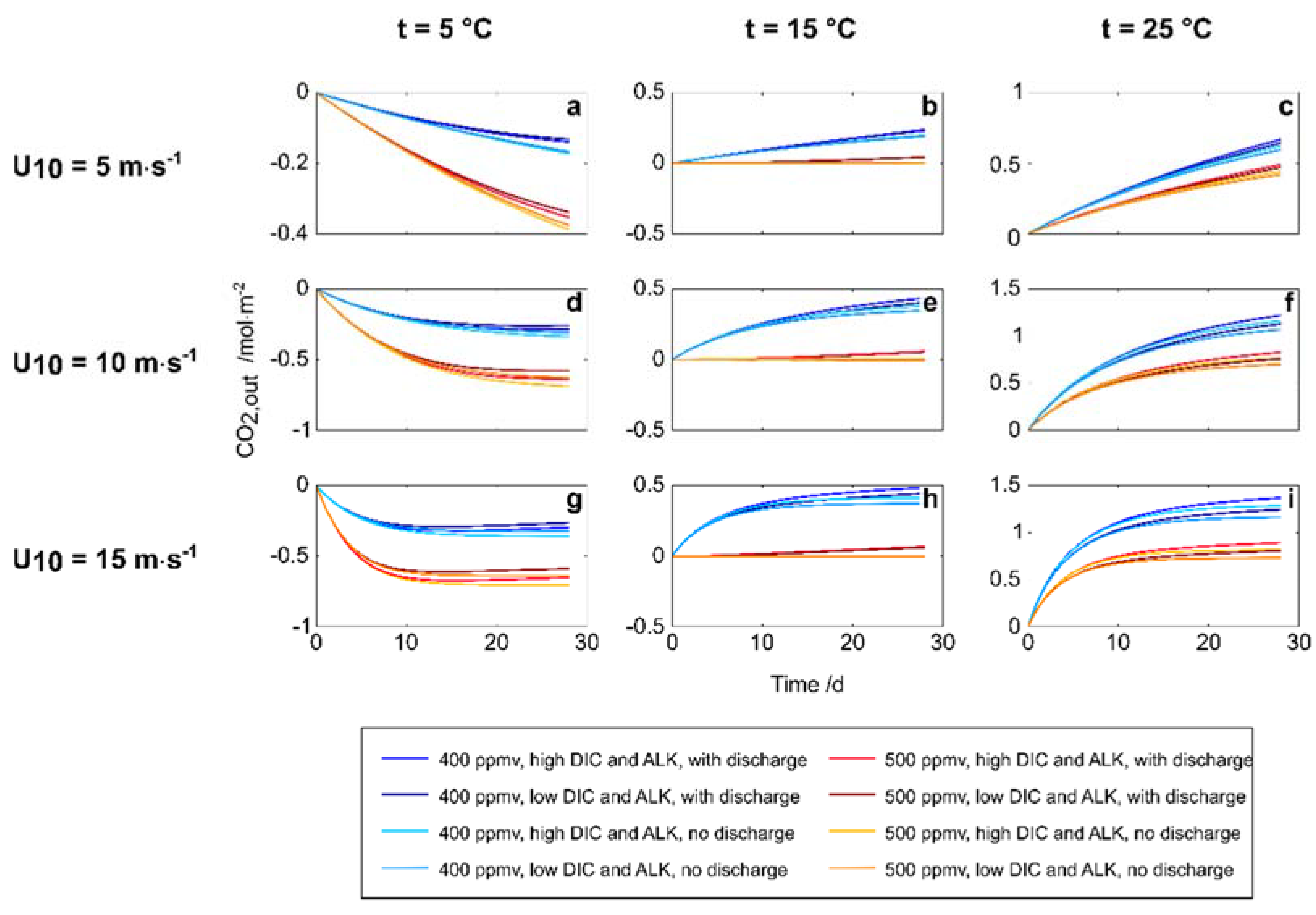
3. Factors Influencing CO₂ Outgassing and Consequences for Putative Discharge Sites

As outlined in Section 2, outgassing of CO₂ plays a critical role in the identification of appropriate locations to discharge AWL-derived water. The flux of CO₂ over the sea surface boundary can be calculated according to:

$$\mathrm{F}=\mathrm{k}·{\mathrm{K}}_0·({\mathrm{fCO}}_{2,\mathrm{w}}-{\mathrm{fCO}}_{2,\mathrm{a}})$$

(2)

where k is the gas transfer velocity, K₀ is the solubility, and fCO_2,w and fCO_2,a are the fugacities of CO₂ that is in equilibrium with the sea surface water and the above lying air, respectively (e.g., [25]). The gas transfer velocity is a function of wind speed and temperature. Wind is not directly forcing the gas transfer, but it affects several processes at the sea surface that do have an impact, e.g., turbulence and shear in the liquid layer, and bubble formation [25]. The solubility of CO₂ depends on temperature and salinity, with the temperature dependency being more prominent [26]. Whether the flux of CO₂ is from air to sea or vice versa is driven by the difference of the fugacities of CO₂ between these two compartments. We analyzed variations in wind speed, temperature, and fCO_2,a, as well as dissolved inorganic carbon (DIC) and TA, which determine the value of fCO_2,w. Wind speed, temperature, DIC and TA values were chosen to cover the variability found in a natural environment. Background values for atmospheric CO₂ represent recent and future CO₂ concentrations. For future CO₂ concentrations, we chose 500 ppmv, which corresponds to the atmospheric CO₂ concentration that is expected to be reached by 2050 in all but one representative concentration pathway (RCP) scenarios. Only in RCP2.6, in which it is assumed that the global greenhouse gas emissions peak around 2020, the atmospheric CO₂ concentration stays below 490 ppmv [3]. Today, it is obvious that this scenario will not hold true. Again, we used the FVCOM-mocsy model setup and applied it on a small test area (Figure S1) to keep the computational demand low. Further information on this setup can be found in the Supporting Information.

At low water temperatures (5 °C), the ocean takes up CO₂ independent of the other parameters (Figure 2a,d,g). The uptake is higher for higher atmospheric CO₂ concentrations. For intermediate temperatures of 15 °C and present atmospheric CO₂ concentrations (~400 ppmv), the ocean loses roughly the amount of CO₂ that is taken up in the 5 °C scenarios (Figure 2b,e,h). At 15 °C and 500 ppmv, almost no exchange of CO₂ between the atmosphere and ocean occurs; the system is close to steady state conditions. If the temperature is further increased, the ocean loses even more CO₂ in the 400 ppmv and is as well losing CO₂ in the 500 ppmv scenarios. This liberating of CO₂ into the atmosphere will in turn contribute to further increasing temperatures. On the other hand, rising atmospheric CO₂ concentrations, which caused the temperature increase in the first place, change the equilibrium CO₂ concentration in the ocean. Higher temperatures can prevail until outgassing of CO₂ occurs. The wind speed is not changing the general pattern of influx or outflux of CO₂. However, it should not be neglected in the evaluation of suitable sites for AWL, e.g., an increase in wind speed from 5 to 10 m·s⁻¹ doubles the amount of outgassed CO₂ within 10 days (Figure 2b,e).

Several conclusions can be drawn from the theoretical assessment of AWL and the sensitivity study. If AWL is applied for a maximum reduction of CO₂ emissions, CO₂ outgassing can be prevented by different strategies. As the mean residence time for deep ocean water is between 1000 and 2700 years [28], outgassing can be completely blocked for the next hundreds or thousands of years, if injections into deep water layers without contact with the atmosphere are performed. This requires additional infrastructure and is worthwhile for large-dimensioned applications only. If AWL-derived water is discharged into upper water layers, it should be discharged shortly after it exits the AWL reactor. Otherwise, once being in contact with the atmosphere, a significant amount of CO₂ would be lost to the atmosphere within a few hours. Generally, mixing with untreated seawater slows down CO₂ outgassing, as it lowers the difference between the oceanic and atmospheric CO₂ concentrations. The amount of CO₂ that is outgassed until equilibrium is reached between atmosphere and ocean does not change, but during the time gained, some of the CO₂-rich water could be transported into deeper water layers. Thus, an injection site where the water mass is rapidly transported towards deeper layers or the open ocean, is favourable in comparison to insulated areas. In addition, an elongation of injection pipes several meters away from the coastline could avoid mechanical stress (turbulence, shear and bubble formation) between the discharged water mass and surrounding rocks and significantly lower CO₂ outgassing.

As illustrated in Figure 2, the water temperature is of major importance and should be as low as possible. Therefore, AWL is best applied north of 40° N or south of 40° S, where annual mean surface water temperatures seldom exceed 15 °C. In some subtropical or tropical regions, colder sea surface temperatures (SSTs) can also be found. This is caused by upwelling of deeper water layers, and SST can be lowered by up to 10 °C (e.g., [29,30]). However, these waters are unfortunately characterized by high pCO₂ values (e.g., [31,32]). As the sea surface pCO₂ far exceeds atmospheric pCO₂ values, a flux of CO₂ from the ocean to the atmosphere is expected and could be verified in several studies (e.g., [33,34]). However, results of other studies suggest that upwelling regions could also be sinks for CO₂, due to a high primary production and associated CO₂ consumption in these systems (e.g., [35,36]). Whether upwelling regions are suitable for the superficial discharge of AWL-derived water must be evaluated on a case-by-case basis. Upwelling is assumed to be limited to water depths of 300 m [37]. Therefore, injections into deeper water layers can be performed independently of the occurrence of upwelling. Estuaries in general are characterized by high fluxes of CO₂ from the ocean to the atmosphere (e.g., [33,38]) and should not be considered for AWL.

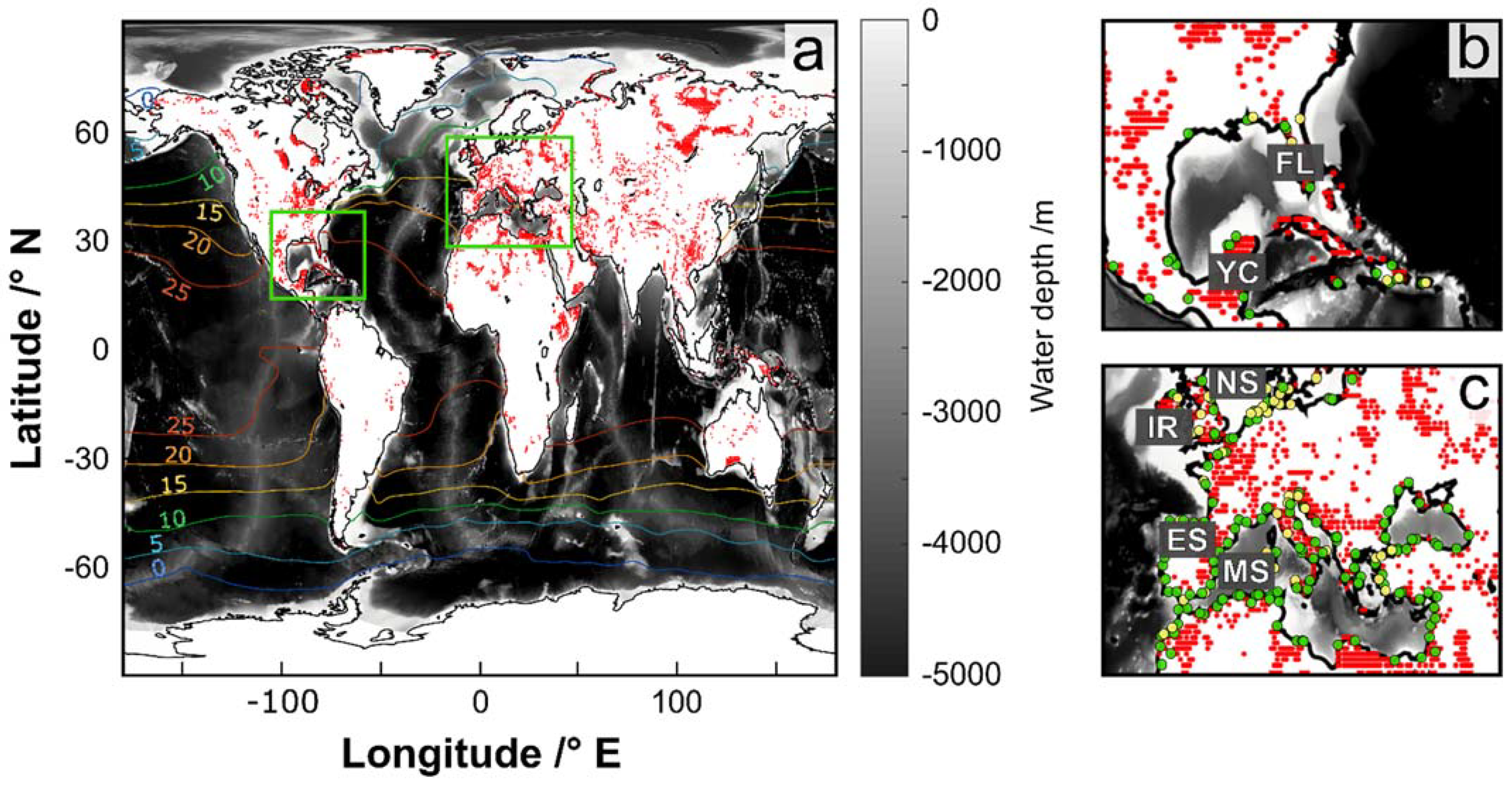
4. Appropriate Locations for AWL

Bhutan and Suriname are among a few carbon-negative countries to date. They committed to remain carbon-neutral at the United Nations Climate Change Conferences in 2009 and 2017, respectively. While 19 other countries likewise pledged to be carbon neutral until 2050 [39], currently, 454 coal-fired power plants are in planning or under construction [40]. Coal-fired power plants have been suggested to be main targets for AWL, as they produce plenty of CO₂ and use huge amounts of seawater for cooling purposes. This water could be reused in AWL [6] to circumvent an additional energy demand for pumping. However, as the associated temperature increase in cooling water is about 10 °C [41], the flux of CO₂ from the effluent gas into the limestone suspension is reduced. Likewise, the dissolution of limestone is reduced because of lower pCO₂ in the limestone suspension, as well as the higher temperature itself. Additionally, outgassing of CO₂ is enhanced once the AWL-derived water is in contact with the atmosphere. For maximum CO₂ emission reduction, we consider this approach to only be reasonable in combination with an injection into deep water layers to prevent outgassing. If the focus of AWL lies on alkalinization of the seawater and not CO₂ emission reduction, using cooling water with increased temperature might even be helpful for the degassing process of AWL-derived water. Then, a discharge into surface water would be possible. In both cases, it should be assured that the discharge/injection takes place in well-mixed areas, as the DIC and TA of AWL-derived water are unnaturally high [12]. To attain maximum mixing, pipes could be designed with several outlet ports along the route into deep water.

Possible locations of deep water injections include, for example, the area around Florida and the Yucatán Peninsula (Figure 3b). Here, limestone is widely available, but water temperatures are too high for superficial discharge. Florida lies within a wide continental shelf, which separates it from the deep ocean. Therefore, the installed pipes must bridge approximately 100 km until deeper water layers can be reached. However, because of the sizeable population of Florida, and thus high CO₂ emissions, pipes with large diameters could be constructed, which are more cost-effective and result in lower costs per sequestered ton of CO₂.

We do not want AWL to be understood as a tool to legitimize the use of fossil fuels for energy generation. However, human energy demand is not expected to decline, and green technologies, such as biogas plants, may replace coal-fired power plants at several locations where they can make use of some existing infrastructure. In addition to the energy sector, the cement industry and waste incineration plants are other large point emitters of CO₂. Smaller amounts of CO₂-rich effluent gas accrue, for example, at combined heat and power plants or wastewater treatment plants. If this effluent gas is treated via AWL, the discharge will presumably be carried out in the upper water layers, as the construction of pipelines for deep injections might not be economically reasonable. The west coast of Ireland could be a suitable location for such superficial applications (Figure 3c). There, the mean SST is below 15 °C, which reduces the outgassing of CO₂. The North Sea is characterized by similar temperatures, but as it has a mean depth of approximately 100 m, transport of AWL-derived water into deeper layers is not possible, and CO₂ outgassing will be high [13]. Generally, appropriate locations for superficial discharge are less abundant than deep water injection sites. If AWL is not applied to sequester a maximum amount of CO₂ but to protect specific areas against ocean acidification, superficial discharge can be performed for all given SST conditions, as the degassing of AWL-derived water was already carried out, and further degassing is not possible. Limestone is a frequently occurring mineral in Europe, available and able to be processed at many coastal sites. In southern Europe, the mean SST is above 15 °C and we recommend deep water injections instead of superficial discharge. The northern coast of Spain is a promising location, as well as several spots along the coast of the Mediterranean Sea, where limestone is available near the coast and the bathymetry sharply deepens towards the open ocean.

Even if CO₂ emissions decrease in the future, mainly due to the substitution of fossil fuels in the energy and transport sectors, a replacement of other CO₂-emitting industries such as cement production or waste incineration is unlikely. For recent and future conditions, AWL might be one part of the overall solution to downsize climate change effects. More research is needed before it can be applied on an industrial scale. A secure application requires more research on (i) the impacts of ocean alkalinization and the combined effect of increased TA but decreased pH on marine ecosystems, (ii) alterations of the marine carbonate systems if applied at a global scale, and (iii) potential side effects, such as a sea level rise owing to the dissolution of millions of tons of limestone in marine environments.

5. Conclusions

Extraction, comminution and transport of limestone liberates CO₂ alongside the operation of AWL itself. If the transportation does not exceed 100 km, these processes reduce the maximum sequestration potential of AWL by only 5%. Depending on the applied process, the characteristics of AWL-derived water can be classified into two categories. At the time it leaves the AWL reactor, it is characterized by a high alkalinity but a low pH value. The highest possible amount of CO₂ is stored in this water, but it is not in equilibrium with the atmosphere. Upon discharge and contact with the atmosphere, a large fraction of CO₂ is outgassed, lowering the CO₂ sequestration efficiency. AWL-derived water can also be actively degassed, leading to pH values which exceed those of the used seawater. Although the CO₂ sequestration efficiency is lower, these waters could help to protect endangered marine environments against ocean acidification. Outgassing of CO₂ is dominated by the difference between the fCO₂ in the atmosphere and the oceanic surface layer, and the SST of the discharge site. High SST can be circumvented by injections into deep water layers to prevent CO₂ outgassing. Worldwide, several locations are promising for either deep water injections or superficial discharge. AWL in combination with deep water injections could be performed in Florida, Yucatán, or around the Mediterranean Sea. Superficial discharge is possible at fewer locations, e.g., in Ireland. If AWL is not applied to sequester a maximum amount of CO₂ but to protect specific areas against ocean acidification, superficial discharge can be performed for all given SST conditions, as the degassing of AWL-derived water has already been carried out.

References

1. Angeles Gallego, M.; Timmermann, A.; Friedrich, T.; Zeebe, R.E. Drivers of future seasonal cycle changes in oceanic pCO2. Biogeosciences 2018, 15, 5315–5327. [Google Scholar] [CrossRef] [Green Version]
2. UNFCC. The Paris Agreement. 2015. Available online: https://unfccc.int/process-and-meetings/the-paris-agreement/the-paris-agreement (accessed on 12 July 2021).
3. IPCC. Climate Change 2014: Mitigation of Climate Change. In Working Group III Contribution to the Fifth Assessment Report of the Intergovernmental Panel on Climate Change; Cambridge University Press: Cambridge, UK; New York, USA, 2014; p. 1435. [Google Scholar] [CrossRef] [Green Version]
4. Walker, J.C.G.; Hays, P.B. A Negative Feedback Mechanism for the Long-Term Stabilization of Earth’s Surface Temperature. J. Geophys. Res. 1981, 86, 9776–9782. [Google Scholar] [CrossRef]
5. Berner, R.A.; Lasaga, A.C.; Garrels, R.M. The carbonate-silicate geochemical cycle and its effect on atmospheric carbon dioxide over the past 100 million years. Am. J. Sci. 1983, 283, 641–683. [Google Scholar] [CrossRef]
6. Rau, G.H.; Caldeira, K. Enhanced carbonate dissolution: A means of sequestering waste CO2 as ocean bicarbonate. Energy Convers. Manag. 1999, 40, 1803–1813. [Google Scholar] [CrossRef] [Green Version]
7. Chou, W.C.; Gong, G.C.; Hsieh, P.S.; Chang, M.H.; Chen, H.Y.; Yang, C.Y.; Syu, R.W. Potential impacts of effluent from accelerated weathering of limestone on seawater carbon chemistry: A case study for the Hoping power plant in northeastern Taiwan. Mar. Chem. 2015, 168, 27–36. [Google Scholar] [CrossRef]
8. Haas, S.; Weber, N.; Berry, A.; Erich, E. Limestone powder carbon dioxide scrubber as the technology for Carbon Capture and Usage. Cem. Int. 2014, 3, 34–45. [Google Scholar]
9. Rau, G.H. CO2 mitigation via capture and chemical conversion in seawater. Environ. Sci. Tech. 2011, 45, 1088–1092. [Google Scholar] [CrossRef] [PubMed]
10. Rau, G.H.; Knauss, K.G.; Langer, W.H.; Caldeira, K. Reducing energy-related CO2 emissions using accelerated weathering of limestone. Energy 2007, 32, 1471–1477. [Google Scholar] [CrossRef]
11. Kirchner, J.S.; Berry, A.; Ohnemüller, F.; Schnetger, B.; Erich, E.; Brumsack, H.-J.; Lettmann, K.A. Reducing CO2 emissions of a coal-fired power plant via accelerated weathering of limestone: Carbon capture efficiency and environmental safety. Environ. Sci. Tech. 2020, 54, 4528–4535. [Google Scholar] [CrossRef]
12. Caldeira, K.; Rau, G.H. Accelerating carbonate dissolution to sequester carbon dioxide in the ocean: Geochemical implications. Geophys. Res. Lett. 2000, 27, 225–228. [Google Scholar] [CrossRef]
13. Kirchner, J.S.; Lettmann, K.A.; Schnetger, B.; Wolff, J.-O.; Brumsack, H.-J. Carbon capture via accelerated weathering of limestone-modeling local impacts on the carbonate chemistry of the southern North Sea. Int. J. Greenh. Gas Control 2020, 92, 102855. [Google Scholar] [CrossRef]
14. Hartmann, J.; West, A.J.; Renforth, P.; Köhler, P.; De La Rocha, C.L.; Wolf-Gladrow, D.A.; Dürr, H.H.; Scheffran, J. Enhanced chemical weathering as a geoengineering strategy to reduce atmospheric carbon dioxide, supply nutrients, and mitigate ocean acidification. Rev. Geophys. 2013, 51, 113–149. [Google Scholar] [CrossRef] [Green Version]
15. Hangx, S.J.T.; Spiers, C.J. Coastal spreading of olivine to control atmospheric CO2 concentrations: A critical analysis of viability. Int. J. Greenh. Gas Control 2009, 3, 757–767. [Google Scholar] [CrossRef]
16. Subhas, A.V.; Rollins, N.E.; Berelson, W.M.; Dong, S.; Erez, J.; Adkins, J.F. A novel determination of calcite dissolution in seawater. Geochim. Cosmochim. Acta 2015, 170, 51–68. [Google Scholar] [CrossRef]
17. Oates, J.A.H. Lime and Limestone: Chemistry and technology, Production and Uses; Wiley-VCH: Weinheim, Germany, 1998; p. 455. [Google Scholar]
18. Renforth, P.; Jenkins, B.G.; Kruger, T. Engineering challenges of ocean liming. Energy 2013, 60, 442–452. [Google Scholar] [CrossRef] [Green Version]
19. Le Quéré, C.; Andrew, R.M.; Friedlingstein, P.; Sitch, S.; Hauck, J.; Pongratz, J.; Pickers, P.A.; Korsbakken, J.I.; Peters, G.P.; Canadell, J.G.; et al. Global Carbon Budget 2018. Earth Syst. Sci. Data 2018, 10, 2141–2194. [Google Scholar] [CrossRef] [Green Version]
20. Felekoglu, B. Utilisation of high volumes of limestone quarry wastes in concrete industry (self-compacting concrete case). Res. Cons. Rec. 2007, 51, 770–791. [Google Scholar] [CrossRef]
21. Renforth, P.; Henderson, G. Assessing ocean alkalinity for carbon sequestration. Rev. Geophys. 2017, 55, 636–674. [Google Scholar] [CrossRef]
22. ECTA. Guidelines for measuring and managing CO2 emission from freight transport operations. Cefic Rep. 2011, 1, 1–18. [Google Scholar]
23. Chen, C.; Liu, H.; Beardsley, R.C. An Unstructured Grid, Finite-Volume, Three-Dimensional, Primitive Equations Ocean Model: Application to Coastal Ocean and Estuaries. J. Atmos. Ocean. Technol. 2003, 20, 159–186. [Google Scholar] [CrossRef]
24. Orr, J.C.; Epitalon, J.-M. Improved routines to model the ocean carbonate system: Mocsy 2.0. Geosci. Model Dev. 2015, 8, 485–499. [Google Scholar] [CrossRef] [Green Version]
25. Wanninkhof, R. Relationship between wind speed and gas exchange over the ocean. Limnol. Oceanogr. Methods 2014, 12, 351–362. [Google Scholar] [CrossRef]
26. Weiss, R.F. Carbon dioxide in water and seawater: The solubility of a non-ideal gas. Mar. Chem. 1974, 2, 203–215. [Google Scholar] [CrossRef]
27. Berry, A.; Kirchner, J.S.; Ohnemüller, F.; Weber, N.; Erich, E.; Brumsack, H.-J. ECO2—Entwicklung des Kalksteinmehl-CO2-Waschverfahrens, Praxisoptimierung und Ökologische Bewertung. Project Report. 2018, p. 165. Available online: https://fg-kalk-moertel.de/files/Forschungsbericht_01_2018_18560N_ECO2.pdf (accessed on 1 November 2021). (In German).
28. DeVries, T.; Primeau, F. Dynamically and Observationally Constrained Estimates of Water-Mass Distributions and Ages in the Global Ocean. J. Phys. Oceanogr. 2011, 41, 2381–2401. [Google Scholar] [CrossRef] [Green Version]
29. Benazzouz, A.; Mordane, S.; Orbi, A.; Chagdali, M.; Hilmi, K.; Atillah, A.; Hervé, D. An improved coastal upwelling index from sea surface temperature using satellite-based approach—The case of the Canary Current upwelling system. Cont. Shelf Res. 2014, 81, 38–54. [Google Scholar] [CrossRef]
30. Marchesiello, P.; Estrade, P. Eddy activity and mixing in upwelling systems: A comparative study of Northwest Africa and California. Int. J. Earth Sci. 2009, 98, 299–308. [Google Scholar] [CrossRef]
31. González-Dávila, M.; Casiano, J.M.S.; Machín, F. Changes in the partial pressure of carbon dioxide in the Mauritanian-Cap Vert upwelling region between 2005 and 2012. Biogeosciences 2017, 14, 3859–3871. [Google Scholar] [CrossRef] [Green Version]
32. Shen, S.G.; Thompson, A.R.; Correa, J.; Fietzek, P.; Ayón, P.; Checkley, D.M. Spatial patterns of Anchoveta (Engraulis ringens) eggs and larvae in relation to pCO2 in the Peruvian upwelling system. Proc. R. Soc. B 2017, 284. [Google Scholar] [CrossRef] [PubMed] [Green Version]
33. Borges, A.V.; Delille, B.; Frankignoulle, M. Budgeting sinks and sources of CO2 in the coastal ocean: Diversity of ecosystem counts. Geophys. Res. Lett. 2005, 32, 1–4. [Google Scholar] [CrossRef] [Green Version]
34. Rosón, G.; Álvarez-Salgado, X.A.; Pérez, F.F. Carbon cycling in a large coastal embayment, affected by wind-driven upwelling: Short-time-scale variability and spatial differences. Mar. Ecol. Prog. Ser. 1999, 176, 215–230. [Google Scholar] [CrossRef] [Green Version]
35. Evans, W.; Hales, B.; Strutton, P.G. Seasonal cycle of surface ocean pCO2 on the Oregon shelf. J. Geophys. Res. Oceans 2011, 116, 1–11. [Google Scholar] [CrossRef] [Green Version]
36. González-Dávila, M.; Santana-Casiano, J.M.; Ucha, I.R. Seasonal variability of fCO2 in the Angola-Benguela region. Prog. Oceanogr. 2009, 83, 124–133. [Google Scholar] [CrossRef]
37. Pond, S.; Pickard, G.L. Introductory Dynamical Oceanography; Elsevier: Oxford, UK, 1989; p. 329. [Google Scholar]
38. Frankignoulle, M. Carbon Dioxide Emission from European Estuaries. Science 1998, 282, 434–436. [Google Scholar] [CrossRef] [Green Version]
39. Declaration of the Carbon Neutrality Coalition. 2018. Available online: www.carbon-neutrality.global (accessed on 6 March 2019).
40. Global Coal Plant Tracker. Available online: https://endcoal.org/global-coal-plant-tracker/ (accessed on 4 March 2019).
41. Langford, T.E.L. Thermal Discharges And Pollution. Encycl. Ocean Sci. 2001, 2933–2940. [Google Scholar] [CrossRef]
42. Hartmann, J.; Moosdorf, N. The new global lithological map database GLiM: A representation of rock properties at the Earth surface. Geochem. Geophys. 2012, 13, 1–37. [Google Scholar] [CrossRef]
43. General Bathymetric Chart of the Oceans: One Minute Grid. Available online: https://www.gebco.net/data_and_products/gridded_bathymetry_data/gebco_one_minute_grid/ (accessed on 18 August 2021).
44. Kalnay, E.; Kanamitsu, M.; Kistler, R.; Collins, W.; Deaven, D.; Gandin, L.; Iredell, M.; Saha, S.; White, G.; Woollen, J.; et al. The NCEP/NCAR 40-Year Reanalysis Project. Bull. Am. Meteorol. Soc. 1996, 77, 437–471. [Google Scholar] [CrossRef] [Green Version]
45. CemNet. Available online: https://www.cemnet.com/global-cement-report/ (accessed on 29 September 2021).
Figure 1. Impacts of AWL-derived water on the pHT of a coastal ecosystem. The application of AWL at a coal-fired power plant, and the superficial discharge of the resulting water, were simulated over a period of four months. Maximum observed changes to the undisturbed system are shown. The area in the red rectangle in (a) is enlarged in (b,c), respectively. (b) Water is discharged directly after it leaves the AWL reactor (pCO2 within the reactor ~120,000 ppmv; pHT = 6.8). (c) Water has been degassed to equilibrium of CO2 with the atmosphere before it is discharged (pHT = 8.6). The arrow indicates the discharge site close to an existing power plant. The color bars have been capped for better visualization.
Minerals 11 01261 g001
Figure 2. Sensitivity study of CO2 outgassing. U10: wind speed in 10 m above the sea surface; t: temperature. Positive values represent outgassing of CO2 from the ocean. DIC and TA in the low DIC and ALK scenario were 2.025 and 2.2 mol·m−3, respectively. Corresponding values of the high DIC and ALK scenario were 2.2 and 2.4 mol·m−3. In scenarios with discharge, 30 m3·h−1 of AWL-derived water (pHT = 6.8) were discharged into the test area. This amount is produced by an AWL demonstration plant [27]. (ai) Amount of outgassed CO2 in dependence of different temperatures and wind speeds.
Minerals 11 01261 g002
Figure 3. Identification of appropriate locations for AWL. (a) Overview of limestone occurrence, water depth and SST. Red: limestone occurrence based on the GLiM database [42]. Bathymetry data on a one-minute grid are from GEBCO [43]. Mean annual sea surface temperatures are from the NOAA Extended Reconstructed SST version 4 [44]. The areas in the green rectangles in (a) are enlarged in (b,c), respectively. Yellow dots: coal-fired power plants according to the Global Coal Plant Tracker [40]. Green dots: a single or several nearby cement plants where limestone waste occurs; according to CemNet [45] IR: Ireland, ES: Spain, NS: North Sea, MS: Mediterranean Sea, FL: Florida, YC: Yucatán.
Minerals 11 01261 g003