
Advances on the Fragmentation-Energy Fan Concept and the Swebrec Function in Modeling Drop Weight Testing


1
Department of Mineral Resources and Petroleum Engineering, Montanuniversität Leoben, 8700 Leoben, Austria
2
ETSI Minas y Energía, Universidad Politécnica de Madrid, 28003 Madrid, Spain
3
Mining Engineering Department, Muğla Sıtkı Koçman University, Muğla 48000, Turkey
*
Author to whom correspondence should be addressed.
Minerals 2021, 11(11), 1262; https://0-doi-org.brum.beds.ac.uk/10.3390/min11111262
Submission received: 2 October 2021
/
Revised: 3 November 2021
/
Accepted: 5 November 2021
/
Published: 13 November 2021
(This article belongs to the Special Issue Advances in Ore Characterization Methods for Comminution)
Abstract
:The breakage index equation (BIE), or model from drop weight testing (DWT) data for rocks and ores is used in the design of crushers and mills. Such models are becoming increasingly difficult to visualize as the number of variables increases. The so-called double fan BIE, combined with the Swebrec distribution’s accurate description of the sieving curves, is applied to the modelling of drop-weight test fragmentation. The key parameters are geometric properties visible in the fan plot; slopes of straight lines and their point of convergence. The ability of the double fan BIE to reproduce DWT data had been previously established for 8 rocks with 480 DWT data sets. Here the fidelity of the double fan BIE is further evaluated for 18 new materials, based on 281 data sets. The fidelity of the double fan BIE with three fan lines is on par with the fidelity of the current state-of-the-art models for the new materials. Besides the breakage index equation, the new double fan BIE’s equation produces, without additional parameters or fitted constants, the general breakage surface equation for an arbitrary value as a bonus. The specific sieving curve for any combination of particle size and impact energy is also contained in the same formula. The result is an accurate, compact and transparent model.
1. Introduction
The mathematical form of the cumulative fragment size distribution (CDF) or mass passing function with being the fragment size, has been the focus of much attention and debate ever since Rosin and Rammler [1] introduced their well-known exponential function (RR) to describe the sieving curves of crushed coal. This equation was e.g., used by Cunningham [2,3,4] to describe the sieving curves of blasted rock. Its two independent parameters, i.e., the median fragment size and the uniformity index , are derived from prediction equations that depend on the rock mass properties, the blasting procedure and the explosive used. This very useful set of equations was called the Kuz-Ram model. It and derivations thereof have seen extensive use in blast engineering. A historical summary is given by Ouchterlony and Sanchidrián [5].
The RR function reproduces the sieving curves well in a central range, say 20–80% of total mass passing but near the top end, > 80% there is no upper boulder limit and at the other end the amount of fines is normally much underestimated. Many researchers have suggested new functions that would improve the fitting ‘fidelity’, i.e., the degree of exactness with which the data are reproduced. In the sequel fitting fidelity will mean the unweighted coefficient of determination in linear space if nothing else is said. One such function is the Swebrec function [6,7], which at the cost of one additional parameter overcomes the two drawbacks of the RR function:
Here, is the largest fragment size and a curvature or undulation exponent. was first used for blasted rock but works equally well for crushed rock. In a series of papers Sanchidrián and coworkers [8,9,10,11] have shown that the Swebrec function nearly always provides higher fidelity fits to fragmentation data than other distributions of comparable complexity.
In order to avoid too much focus on the mathematical form of the CDF, Sanchidrián and Ouchterlony [12] presented a blast fragmentation model () that did not explicitly presume such a function, even if the Swebrec function provided some help in the derivation. During that work it was realized that the Swebrec function had an interesting property called the fragmentation-energy fan [13]. In short this means that (a) if the fragmentation data follow Equation (1) with and with the specific charge, then (b) when plotted as vs. for arbitrary values of the data will form straight lines, with slopes depending only on , and these lines will converge on a focal point that depends on the blasted material. See Figure 1 below as an example.
A logical next step was to use the properties of the Swebrec function to analyze the crushing of rock. More specifically to analyze the so-called drop weight testing (DWT) which the Julius Kruttschnitt Mineral Research Centre (JKMRC, often JK for short in this paper) has spent so much effort to develop methods for, see [14,15,16,17,18,19,20] e.g., and to use in crusher and mill modeling. In 2018, Ouchterlony and Sanchidrián presented a new form of analysis of the DWT data [21], that was able to represent the breakage space based on the Swebrec description of fragmentation.
Figure 1.
Fragmentation-energy fan; sieving data from blasted cylinders of Hengl amphibolite (Figure 2 in [21]) plotted as: . Crossed points not included in the fits.
Figure 1.
Fragmentation-energy fan; sieving data from blasted cylinders of Hengl amphibolite (Figure 2 in [21]) plotted as: . Crossed points not included in the fits.

The DWT yields initially sieving curves for the progeny generated from particle sizes impacted by a falling weight and their dependence on the specific impact energies (kWh/tonne). A key parameter extracted from the DWT is , the cumulative percentage passing 1∕10th of the initial particle size . Its dependence on , is called a breakage index equation (BIE), and it is a measure of the high-energy impact breakage taking place in crushers and AG/SAG mills. The JKMRC has a long history in the development and use of the DWT [22].
The DWT data are also used to construct, through interpolation a set of -values where = 2, 4, 10, 25, 50 and 75 and is the amount of material passing a sieve opening -th of the original particle size. Let describe the cumulative distribution function. Then may be expressed as:
This equation shows that having a set of interpolated data for relevant combinations of and amounts to knowing the corresponding sieving curves. One of the most extensive available data series on laboratory drop weight testing (DWT) of particles of rock, mostly ores, is found in the thesis of Banini [19] from the JKMRC. Fits to Banini’s [19] data showed that judged by the -values, the Swebrec function does an outstanding job of fitting the sieving curves, the median coefficient of determination for a weighted regression in linear space was = 0.997–0.999 [21]. See also Table 3 below.
Using normalized size data and scaled energy data, and , where is an arbitrary reference size and a scaling exponent and fitting parameter, Ouchterlony and Sanchidrián [21] in a preliminary analysis with the linear fan derived the following equation for for Banini’s [19] Mt Coot-tha hornfels data.
Here, and refer to the approximate position of the focal point in Figure 2 and and denote the (negative) slope values of the and lines in the figure. The undulation exponent was calculated from and .The best energy scaling was achieved by choosing . mm suited the range of particle size fractions used by Banini [19], from to mm. In the derivation, the geometric means of the bin range limits were used. The corresponding breakage index equation curve is shown in Figure 3.
The agreement between Equation (3) and the data is good, = 0.977, computed in linear space. Note that all five parameters in Equation (3) are directly related to the geometry of the fragmentation energy fan in Figure 2 and to the Swebrec function in Equation (1), which also determines the mathematical form of Equation (3). Note also that there is a “hidden”, sixth scaling parameter λ in Equation (3). Note finally that the corresponding equation for any other -value directly follows, Equations (18a,b) and (25) in [21]:
The fitted functional form of used by Banini [19] gave a better result than the linear fan, = 0.988. The functional form used by Shi and Kojovic [22] and Shi [20], see Equation (6) below, gave an even better result = 0.993. See Table 2 in [22]. The main reason is that the high-energy data in Figure 3 follow a different trend than the low-energy data. The fitting parameter in Equation (6) accounts for this. Refined fitting procedures [21] with the linear fan gave the data in the first row in Table 1 for Banini’s [19] rocks. Shi and Kojovic’s [22] data in row 2 are here to referred to as ‘JK new BIE’ (breakage index equation). These data are all higher.
The deviating high-energy trend in Figure 3 is, to a lesser extent, also visible in the fragmentation-energy fan in Figure 2 and in all the corresponding diagrams for Banini’s rocks. To include this trend in the analysis the double fragmentation-energy fan was introduced [21]. It consists of a primary fan; a set of fan lines with a common focal point valid for the low-energy region where is the energy measure, and a secondary fan with a different focal point for the high-energy region . At the fan lines are connected in such a way that the primary fan lines have a change in their slope values or kinks as shown in Figure 4.
Figure 2.
Normalized percentile fragment sizes vs. scaled impact energy data from DWT, showing fragmentation-energy fan behavior (Figure 4 in [21]).
Figure 2.
Normalized percentile fragment sizes vs. scaled impact energy data from DWT, showing fragmentation-energy fan behavior (Figure 4 in [21]).

Figure 3.
Breakage index equation , Equation (3), for Mt Coot-tha hornfels, based on fragmentation energy fan (Figure 5 in [21]). Note that the non-linear regression that determined the fan parameters was made in the log-log space of Figure 2 whereas for the fan equation was obtained without any regression by comparing the resulting equation with the data in linear space.

Figure 4.
A double fragmentation-energy fan, with kinks on the fan lines at . P1, P2, P3 are percentage passing, P1 > P2 > P3.
Figure 4.
A double fragmentation-energy fan, with kinks on the fan lines at . P1, P2, P3 are percentage passing, P1 > P2 > P3.

The secondary fan has a different focal point but the undulation exponent doesn’t change. There are now nine parameters; six from the primary fan plus three new ones, the focal point of the secondary fan and the kink position . Formulas for the double fan were derived and the effect of using different numbers of fan lines in the fitting process was tested. Five fan lines, e.g., = 80, 65, 50, 35, 20% or = 90, 70, 50, 30, 10%, seemed to be the optimum but three fan lines gave nearly as good a fidelity.
The improved results for the double fan are shown in Figure 5 and the last row of Table 1. The values for the double fan equations are higher than the JK new BIE ones [20,22] for three of the eight rocks. The corresponding breakage surface is shown in Figure 6.
Figure 5.
Double fragmentation-energy fans (a), and breakage index equations of the scaled impact energy (b) for Mt Coot-tha hornfels. Circles are data points. Solid and dashed lines in (a) are primary and secondary fans, respectively ([21], Figure 14). Colors indicate different percentiles: blue—90%, red—70%, yellow—50%, purple—30%, green—10%.

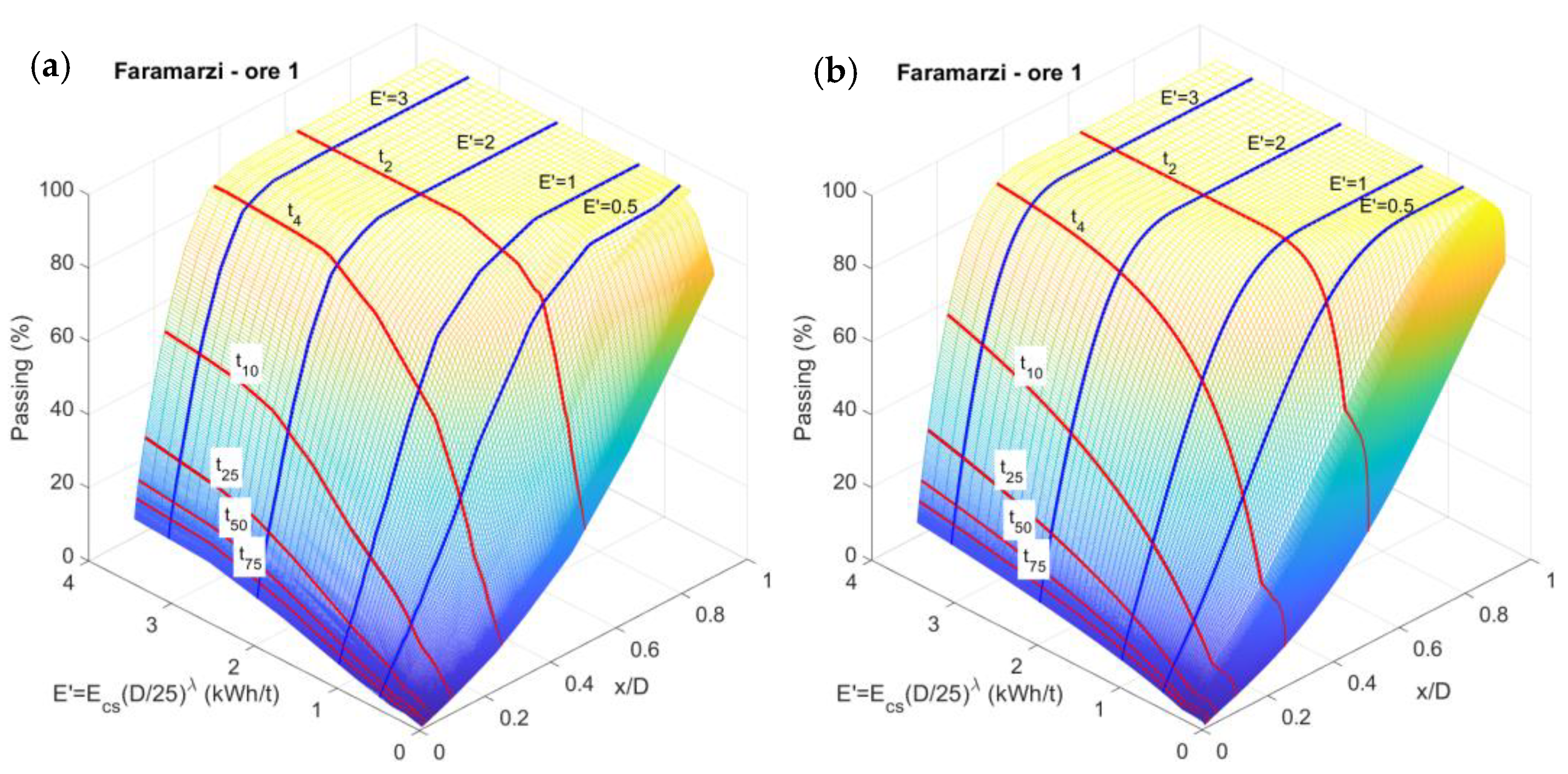
Figure 6.
Breakage surfaces for Mt Coot-tha hornfels as predicted from the double fan fits (a) and the Banini [19] data (b). The lines shown are size distributions for a scaled crushing energy of 1.5, 3 and 6 kWh/t (blue lines), and the breakage indexes and (red lines) ([21], Figure 15).

A detailed analysis of Banini’s DWT of eight rocks using the new fragmentation-energy fan concept is presented in [21]. General breakage surfaces are calculated for all of them, with determined by the Swebrec function. From these the general set of breakage energy curves follow, and more specifically the breakage index equation .
In the discussion of [21], the fragmentation-energy fan method is compared with Banini’s [19] analysis and JKMRC’s size-dependent breakage model [22]. It was said that:
- Banini [19] needs the interpolation splines data to obtain plus 14–18 parameters to determine in his first analysis. When he introduces the size scaling he needs, instead, 3 parameters plus the splines data. Shi and Kojovic [22] need the splines data plus 4 parameters; , , and . With this they obtain a higher fidelity.
- The basic, linear fan method needs 6 parameters to describe ; namely the size scaling exponent , the position of the focal point , the two slope values and plus the Swebrec exponent . Calculating the last two parameters via the slope values and is better. These parameters follow from the fan fitting though, but the fidelity is not as good as that of the JK new BIE [22].
- The double fan method needs the 6 parameters for the primary fan plus the focal point of the secondary fan and the energy value of the kink point, in all 9 parameters but no splines data because and derive from the same function. The fidelity is now almost good as that of the JK new BIE.
- The size scaling of the impact energy in the fan method is more transparent than that used by the others since it lets the scaled energy retain the same units as the impact energy , [kWh/tonne].
- The fan method uses the -values directly or values interpolated from the sieving curves. This loses less information than converting them to -values based on a Rosin-Rammler interpolation.
- The fan method contains information not only on but also on for arbitrary values of . This makes the use of the interpolated representation unnecessary.
Another way of saying this is that the fan method (i) uses fewer and more meaningful parameters, (ii) is more compact and (iii) is more general than the other methods. Yet its fidelity is almost as good.
The work [21] was based on interpolated data from only one source. In this work DWT sieving data from several new sources are analyzed directly, thus widening the experimental basis for the fragmentation-energy fan method. This includes, see Table 2, data from [23,24,25,26,27]. The PhD thesis by Yu [26] contains the sieving data analyzed in [28], that was not available when [21] was drafted. The fan based method can now be compared with Yu’s [28] new 4D-m and 4D-mq models. Some DWT samples data were discussed in [24]. Faramarzi et al. [29] summarize parts of his PhD thesis [27].
Banini’s [19] data mostly concern sulfide ores, see Table 2. The range of materials now also includes cement raw materials such as limestone, clinker (nodules of sintered limestone-aluminosilicate mixtures), trass (volcanic, trachytic tuff), gypsum (hydrated calcium sulfate), salt and clay. Avsar’s [23] materials came from the Yibitas-Lafarge cement plant in Turkey. Genç et al. [24] add the colemanite ore (calcium borate) and quartz but their origins are not specified. Yu [26] adds a gold porphyry ore from Newcrest’s mine Cadia East. Faramarzi’s [27] ores are not described in any detail.

Table 2.
Material types and sources of sieving data for DWT.
| Author | Material Type |
|---|---|
| Banini [19] | hornfels, Cu-ores (2), Pb-Zn ores (3), Au-ores (2) |
| Avsar [23] | cement clinker and trass |
| Genç et al. [24] | cement clinker (2), clay, colemanite, copper ore, gypsum, limestone, quartz (2) and trass |
| Genç [25] | salt ore |
| Yu [26] | Au-Cu porphyry ore |
| Faramarzi [27] | ores 1–4: 1—hard, fresh basalt, 2, 3—hard and 4—soft |
2. Data and Analysis
2.1. Available Sieving Data
The DWT data provided by [23,24,25] were obtained with in-house equipment manufactured to replicate the JK procedure outlined by [18]. Banini’s [19] data were obtained with JK equipment in the JK laboratories, as were Yu’s [26] and Faramarzi’s [27] data.
Napier Munn et al. [18] indicated the use of a testing matrix of 5 specimen sizes (13.2–16 mm up to 53–63 mm) × 3 energy levels that vary with the size in the interval 0.1 to 2.5 kWh/tonne for AG/SAG mill modelling. Banini [19] used larger testing matrices of up to 8 particle sizes (4.75–5.6 mm up to 75–90 mm) × up to 9 impact energy levels (0.02 to 10 kWh/tonne). Avsar [23] used 8 sizes (6.4–9.5 mm up to 44.5–57.2 mm) × 4 energy levels from 0.05 to 3.45 kWh/tonne). Genç [30] used 7 size fractions (4.75–5.6 mm up to 16–22.6 mm) × 3 energy levels from 0.19 to 5.51 kWh/tonne and she used 9 size fractions (4.75–5.6 mm up to 55–62 mm) and mostly 3 energy levels per size fraction in Genç [24].
Faramarzi [27] extended the standard JK DWT testing approach in that he did not merge the progeny of all particles of a given size fraction to calculate average and values. He evaluated and for individual particles to obtain measures of their variability in order to better understand how the intrinsic heterogeneity within an ore domain affects the SAG mill performance.
In the repeatability tests, Faramarzi [27] first tested 30 particles of sizes within the fraction 37.5–45 mm at each of the 3 energy levels, 0.1, 0.25 and 0.5 kWh/tonne, for four ores. He then repeated this test matrix and found an acceptable repeatability. To obtain the comminution percentile curves (breakage index equation) , he then extended the matrix to testing of 30 particles in fraction 19.0–22.4 mm at each of the 6 energy levels 0.5, 1.0, 2.0, 2.5, 3.0 and 4.0 kWh/tonne for three of the ores. For ore 2 he also tested particles in the 16–19 mm fraction at the five lowest of these energy levels.
The work of Yu [26], also reported in [28], aimed to extend the breakage sizes used in standard JK DWT to much finer particle size classes, down to 0.425–0.5 mm. He first tested 5 particle sizes (13.2–16.0 mm to 53–63 mm) at the energy levels 0.1 to 2.5 kWh/tonne. He used the mini JKDWT to test 8 particle sizes (0.425–0.5 mm to 13.2–16.0 mm) at each of the 6 energy levels 0.1, 0.5, 1.0, 1.5, 2.0 and 2.5 kWh/tonne. For the 2 largest of these size fractions a single particle was tested each time, for the 3 smallest a “disperse monolayer of particles” was used with special efforts to distribute their loading evenly. For the 3 intermediate size fractions Yu et al. [28] tested both single particles and disperse monolayers with from 3 to 2000 particles.
Two ways of testing were analyzed [26,28] and it was found that the difference is small for the 3.35–4.0 mm size fraction and that “the results of dispersed monolayer multiple particle breakages for −2 mm were combined with the outcomes of single particle breakage for +2 mm to derive the wide range appearance function”. These are in all probability the sieving data presented in [26]. Based on them Yu developed the 4D-m and 4D-mq appearance function models.
2.2. Analysis of Sieving Data: Formulation of Breakage Index Equations
The fidelities of the following equations will in this paper be compared in terms of in linear space, and in one case in terms of the RMSE:
2.2.1. The Earlier Standard JK DWT Analysis
The breakage index equation is given the following form in which parameters and are presumed material constants
The product , given by the slope at the origin, characterizes the crushability of the rock (ore), and it is also used in the JK crusher models. Equation (5) is independent of particle size. may be determined by interpolation of the sieving data, and by regression. Equation (5) is included for historical reasons.
2.2.2. The JK Size-Dependent Breakage Index Equation or the JK New BIE
Shi and Kojovic [22] developed a size-dependent variant of Equation (5):
See also [20]. Here (%) is the maximum attainable level of . (m) = (mm)/1000 is the initial particle size, (kg/(Jm)) is the material breakage property, the number of impacts (here = 1), (J/kg) the DWT impact energy and a threshold energy for breakage to occur, a fitting parameter. is also a fitting parameter as is the exponent , which is material specific and said often to lie in the range 0 - 1. The particle size in Equation (6) has units (mm). Again, may be determined by interpolation of the sieving data, and by regression. Equation (6) is called “the JK new BIE” in this paper.
2.2.3. The Banini-Bourgeois Size-Dependent Breakage Index Equation
To incorporate the observed size dependence directly into the equation Banini [19] used an equation from Bourgeois ([31], Equation (4.2)) that he modified somewhat so that (note that in Equation (6) does not tend to 100 when ). Here (kWh/m3) is the volume specific impact energy and (kg/m3) is the rock density.
Again, may be determined by interpolation of the sieving data, and by regression. The fitting fidelity for Banini’s rocks was marginally worse than for using Equation (5) with one pair of values for each particle size [21].
2.2.4. The 4D-m and 4D-mq Model Equations
These are defined in Equations (7), (10) and (11) (4D-m) and in Equations (12), (13) and (11) (4D-mq), of Yu et al. [28] plus a couple of tables and their Figure 19. For the present purposes they can be summarized in the following equations:
References [26,28] give the mathematical forms of the rather complex functions and . and denote the top particle size and top impact energy used in the DW testing. The nine Greek symbols denote rock or ore specific parameters. Further is a parameter that is defined in their Figure 19 [28]. The simpler 4D-m model differs in that and that the -parameters take on different values but the -parameters retain the same values.
A comparison with Equations (5)–(7) shows that Yu’s model equations are more general. They make it possible to compute not only by entering into Equation (8a–c) but also by entering . The models are not easy to use though because:
- The Greek - and -parameters are not pure material parameters, they were calibrated for specific ranges of particle sizes and impact energies for the Cadia ore. Even for that material, what happens when the top particle size and top impact energy change is not known, nor what happens when the material changes.
- The procedure used by Yu to determine the - and -parameters is not described in sufficient detail; a “cut-and-trial” fitting method is mentioned, but only vaguely described.
- Yu ([26], p 133) appears to use the geometric mean to characterize particle and progeny size associated with the progeny mass passing. The upper bin limits seem more appropriate.
- Before Equation (14), Yu et al. ([28]) seem to mean that they, apart from 45 cases of bottom sieves have mass passing data for all 20 sieving bin sizes for all 59 progeny CDF, i.e., 1180 − 45 = 1135 data points. The data tables in his thesis, pp 202–205 [26] have only 745 entries including the points . To add dummy points to the curve fitting could have deleterious effects.
These items indicate a large risk of making mistakes when trying to emulate Yu’s derivations for the new materials in this study. Therefore, the comparison of the fidelities of the fragmentation energy fan equations with the results for his Cadia ore data will be restricted to the best fan equations.
2.2.5. The Fragmentation Energy Fan Equations
The first fitting is, in this case, not made to the -equation, such as Equations (5)–(7), or to the mass passing data, like Equations (8a–c), but to the fan line structure of the data that appears when the normalized percentile size vs. the size-scaled impact energy is plotted in log-log scale. See Section 1 and Figure 2, Figure 4 and Figure 5 above. From this analysis for arbitrary values of follows automatically.
Based on the experience in [21], either three fan lines for percentiles or five fan lines for percentiles % are chosen for the fitting. For simplicity dropping the suffix in the mass specific impact energy, i.e., letting then the fan data are fitted by the double fan equations
E’ being the energy scaling equation:
Equations (9a,b) are valid for . Here suffix denotes the primary, low-energy regime fan in Figure 4 and suffix the secondary, high-energy regime fan. denotes the kink energy in Figure 4, denote the low-energy focal point and the slope of fan line in the low-energy fan. The equivalent high-energy fan symbols have suffix instead of .
Here the high-energy fan line slopes are not free parameters, but related to by the fan conditions in the high energy regime and the continuity at .
To these parameters; one slope for each low-energy fan line, two coordinates for the low-energy focal point, the kink energy and the two coordinates for the high-energy focal point, the energy scaling exponent must be added. For the three-line fan this makes 9 independent parameters, and for the five-line fan, 11 parameters are made. Note that the reference size or is arbitrary and doesn’t influence the fitting.
The parameters and in the Swebrec function are e.g., given by three fan line slopes through
When using the Swebrec-derived functions Equations (3) or (4), or Equation (13) below, the number of percentile lines used for the fan fit (that obviously increases the number of unknowns in the fit, as more slopes have to be calculated) does not turn into an increased number of parameters in the breakage model, since this only needs two slopes ( and ) and the Swebrec exponent b. The rest of the slopes (not needed for the breakage functions) can be obtained from these three parameters or from any three slopes. This means that the double fan model can always be fully formulated with 9 parameters.
When the parameters in Equations (12a–c) are known, Equations (11a–c) give the high-energy -values and the focal point is known from the fitting. Note that takes the same value for the low- and high-energy region fans. Equation (4) above gives the generalized breakage index, or breakage surface equation that, for the double fan is:
If is set to 10, is obtained.
The regression fitting was made to minimize the squared errors in Equation (9a,b), i.e., in log-log space. The necessary are generated by linear interpolation in log-log space of the data from the sieving to the appropriate interpolated -values for the fan lines [13,21]. Multiple minimization jobs are performed with different initial points in order to ensure, as far as one can, a minimum of the least squares function.
Three minor developments of the fan based approach have been made to try improve the fidelity of its calculation. Firstly, that a minimum of the specific impact energy is required to achieve breakage may be argued. This changes the energy scaling equation to
This raises the independent parameters in the double fan by one to 10.
Secondly, has been allowed to vary with the particle size. A study of Yu’s [26] data indicates that this would be beneficial, and it is well-known [32] that the size exponent of energy-size relationships varies with particle size. The following function was chosen
and are the small and large particle size limit values of , respectively. Equation (15) allows for a sharp transition from the two λ values if the shape constant is high, or a smooth variation if is small. Such variable lambda calculation involves three more fitting parameters than the basic nine for the double fan; a second level, a dimensionless shift diameter and the shape constant .
Thirdly, originally the percentiles were chosen for the three-line fan fitting, and % for the five-line fan fitting. This spreads the fan-line crossings relatively evenly in the direction and (hopefully) the associated errors. One way of focusing more on the data is to choose the fan percentiles in the range of the measured values.
2.3. Size Distributions of Sieving Data: Swebrec Function Fitting
A successful fragmentation-energy fan is contingent on the Swebrec function parameter being dependent only on the material tested, not on the energy level nor on the particle size. For the linear, single fan, the slope parameters are subject to the same independence restrictions and for the double fan takes on different but related values in the low- and high-energy regimes. The single -value in Equation (13) should thus ideally represent all sets of the sieving data. Due to the natural variability of e.g., particle shapes and material properties this is never the case. Each fit to a sieving curve generates a unique -value.
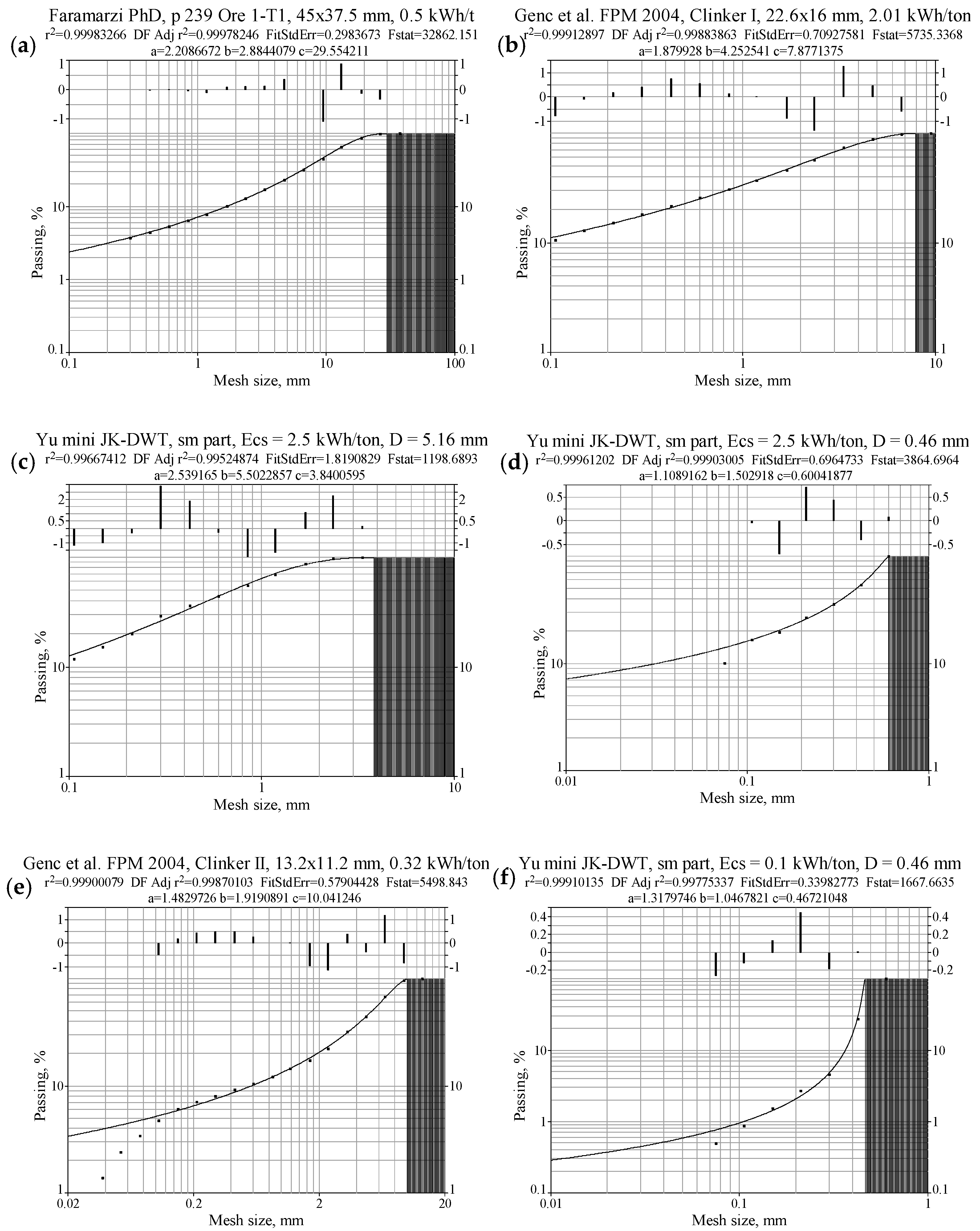
It is thus of interest to know both how well the Swebrec function fits each sieving curve, as expressed e.g., by or another fidelity measure, and how much varies over the whole set of sieving curves. Table 3 shows a summary of the fitting. It was made with the commercial code TableCurve2D, using weighted nonlinear regression in linear space and the weighting function . In some cases, the values were excluded due to their more approximate nature. In some cases, the values were excluded because of a strong downward trend in the fines end of that the three parameter Swebrec function can’t capture and nor can the RR function. Ouchterlony [33] discusses some of the fitting details.
The sieving data display of course a high end cut-off and in general also an upward concavity in the lower medium size range in log-log sale that is characteristic of the Swebrec function but which neither the original nor the rescaled RR function [9,10] can reproduce, both being linear in that range. In a few cases the original RR function seems to do as good a, maybe even better, fitting job than the Swebrec function but as the sieving curves as a whole display the fan character the Swebrec fit is preferred. For small particles the sieving data are in general more irregular, and it is difficult to say which functional dependence is the better one. The six fitting examples in Figure 7 illustrate some of these points.
Table 3 shows that the fitting fidelity of is high. Since = 1 can’t be exceeded and the data are very close to one, the values are presented as a range plus the median. Except for Yu’s [26] Cadia ore and Banini’s [19] Big Bell ore, no -values fall below 0.99. For all data in Table 3, in only 5.5% of the cases. This is almost exactly the estimate 5% made for blasted rock in [7]. The overall median of the median values is 0.9990 and their range is 0.9971–0.9999.
The undulation exponent has no known upper theoretical limit so the values given in Table 3 are the range, the mean and the standard deviation for each material. The data set size weighted mean -value is 2.27 and the mean value for Banini’s data (2.27) is the same as that for the new data (2.27), if the outlier data for Genç’s et al. [24] gypsum (a very soft material compared to the other cement additives, limestone and trass, and the selected drop energy levels for it were very high, which gave a very fine DWT product [30]; the net particle size effect would therefore be difficult to observe, which may the reason for anomalous -values) and one quartz value are removed. The standard deviation for Banini’s mean -values is however almost twice as high, 0.56 compared to 0.31 of the new data. The range of the mean -values is 1.49–4.11 and only six -values fall outside the range 1.75–2.75. Looking at the individual materials gives a much larger range of -values, about 0.9–4.3. They tend to decrease with decreasing particle size and decreasing specific impact energy.
One important question is how such a range of -values can be represented by a single value when deriving the fragmentation energy fan and the connected breakage index equation and ditto surface. Since this was quite successful for Banini’s data, one may expect a similar and probably better result for the new data since the scatter in the -values are smaller. Of the new rocks, Yu’s [26] Cadia gold ore and Genç’s et al. [24] Cayeli copper ore have the largest scatter in the -values, but the number of sieving curves is radically different, 59 vs. 4.
3. Fragmentation-Energy Fans and Breakage Index Equations for New Materials
3.1. Basic Double Fragmentation-Energy Fans for New Rocks
Figure 8 shows some examples of the double three-line fans obtained from the fitting to the interpolated sieving data and for the new materials in Table 2. Fans for the rest of the materials are given in Appendix A. Table 4 compares the -values, from the fan fitting to a set of sieving curves with the average -value, from the Swebrec fitting to each curve in the set.
The average -values from the individual fittings are for all materials except Avsar’s [23] clinker and Genç’s et al. [24] quartz II larger than the fan fitting values, and the difference is in that sense quite consistent. The relative difference is about 15% independent of the -value. At least part of the reason lies in how the fitting was performed; for in linear space with a particle size weighting that favors small sizes and -values whereas for the smallest directly accounted for -value is 20%. and are not nearly as sensitive as (and ) and it is possible to express the Swebrec function in terms of them instead of in terms of and . In one CDF case where weighting vs. no weighting was tried and data at the upper and lower ends of the data range were either omitted or included, the scatter in the -value was 26% and that in and respectively 1.2%, 1.5% and 4%. As long as the fitting conditions are consistent, a -value can be compared with a -value and likewise for .
3.2. Basic Breakage Index Equations
Table 5 shows a comparison of the fidelities of fitting the different breakage index equations (BIE) given in Section 2.2, Equations (6) and (7) plus the effect of using the fitted fragmentation energy fan parameters (Equations (9)–(11)) in Equation (13a,b) with 10 and calculating in vs. space. See, also, graphs in Figure 9 belowand in Appendix B. For the size dependent JK new BIE [22] both positive and negative values for the parameter plus zero were tested. If is allowed to be negative it ceases to have an immediate physical meaning since zero imparted impact energy would result in breakage. The Banini [19] BIE is fitted using impact energy per unit mass although the original function in Equation (7) is written with impact energy per unit volume . The reason is that only the densities of Faramarzi’s [27] and Yu’s [26] rocks were known. A limited trial with = 2.8 tonne/m3 had no systematic effect on , in some cases it increased, in some it decreased. These changes meant, in no case where Banini’s BIE was the best scoring, a different ranking.
There are 18 data sets in Table 5, one row for each material. If negative -values are allowed, then the JK new BIE gives the best fidelity for 11 materials, the Banini BIE for 3 and the fragmentation-energy fan (double fan) BIE for 4 materials. If only positive -values, or zero, are allowed, then the JK new BIE is best for 7 materials, the Banini BIE for 4 and the double fan for 7 materials. In a pair-wise comparison of the -values the JK new BIE gives a higher fidelity than the double fan BIE for 13 of the 18 materials when negative -values are allowed and for 9 of the 18 materials when they are not allowed. Considering the median -values instead, the JK new BIE scores the highest when negative -values are allowed (0.9788). The double fan BIE scores 0.9763, the Banini BIE scores 0.9770 and the JK new BIE the lowest (0.9704) when only positive -values, or zero, are allowed. It seems natural to rank the BIEs as follows: JK new (any ) > Banini ≈ double fan > JK new () even if a pairwise comparison of the values would say that the differences between these BIEs are insignificant on a 0.05 level.
Figure 9 shows BIE curves for two rocks where different BIE give the best fidelity. More examples are given in Appendix B. The fidelities of the different BIEs look much the same but there are some differences in the curves:
- The JK new BIE is the simplest in the sense that the curve is always convex (up) in the plotting space but it levels out below 100% and is questionable.
- The Banini BIE levels out at 100%. It is convex for the most part but turns concave near the origin, a fact that is probably due to the logarithmic abscissa.
- The double fan BIE also levels out at 100% and the curve has a kink, which e.g., could be caused by a change in breakage mode but that remains to be proven.
3.3. Improved Double Fragmentation-Energy Fan BIE
The different ways of improving primarily the fidelity of the (basic) double fan BIE that were discussed in Section 2.2 plus a direct fit solution will be analyzed here, namely:
- I-1.
- 3 fan lines ( = 20%, 50%, 80%), constant plus an -value, 10 parameters.
- I-2.
- 3 fan lines ( = 20%, 50%, 80%) plus varying but no , 12 parameters.
- I-3.
- 5 fan lines ( = 20%, 35%, 50%, 65%, 80%) plus varying but no , 12 parameters.
- I-4.
- 5 fan lines with -values inside the range of measured -values plus varying but no , 12 parameters.
- I-5.
- Direct fit of whole mesh size-passing-sample size-energy space with the equivalents to Equations (13a,b):
Here, the and scaling, and the variable lambda option, of course, are identical to those in the BIE versions. Putting (i.e., ) yields . As with the fan fits, this formulation includes 12 parameters with the variable option without , or 10 with the constant and option.
With improvements I-1 to 3 the generality of the double fragmentation-energy fan approach to DWT analysis is kept, the Swebrec based fan fitting gives the result Equations (13a,b) or (16a,b) for , valid for arbitrary -values and with as a special case. With I-4, the expected result is an improved -value for but at the expense of a poorer fidelity when 10. With improvement I-5, the regression is made neither in the fan space nor in the but in the whole space, directly on DWT sieving data without the recourse to interpolation to derive the percentiles, which is used in the fans formulation. Two versions of I-5 have been analyzed and for them the RMSE or SE (root mean square or standard error) has been used as the fidelity measure so as to make the comparison with Yu’s [26] methods possible.
Table 6 shows the results. The essential information from Table 5, i.e., which BIE that worked best for each material and the corresponding -values are given in the first two columns. The bold numbers in the first column and in the columns for I-1, I-2 and I-3 give the max fidelities up to that point.
Table 6 shows that making improvement I-1 with ≥ 0 for the basic double fan BIE gives a very slight fidelity improvement compared to the JK new BIE (symbol JK E ≥ 0) for one material only, ore 2, and one more against the Banini BIE, limestone I. Allowing < 0 favors the double fan against the JK new BIE for one more material, ore 1, and further improves limestone I. Making I-2, a variable , improves on the fidelities of the basic double fan BIE for two materials, clinker I and quartz I, but doesn’t change the overall top position of the JK new BIE as judged from the median . Making I-3, 5 fan lines and a variable, improves on the double fan BIE fit for two materials, clinker II and Cu ore, on the JK new BIE fit for Cadia ore, and on the Banini BIE fit for trass.
Some detailed observations: Implementing improvements, I-1 to I-3 makes a version of the double fan BIE score best for 9 materials out of 18, vs. 8 for the JK new BIE. The Banini BIE scores highest for one single material, gypsum. The fidelities achieved by making improvement I-4, which involves using percentiles that are adapted to the measured -values, are shown in the next column. This double fan BIE scores best for 6 materials, see the bold numbers, the double fan with I-1 for 3 materials, with I-2 for 2, with I-3 for one material, the Banini BIE for no material and the JK new BIE still scores best for 6 materials.
The bar chart in Figure 10 illustrates the overall behavior of the different BIEs in a more compact way, neglecting the outliers. As expected, the increasing number of parameters in I-1 to I-4 on average leads to an improvement of the fidelity of the double fan fit. It is important to note that the value with which the calculations are qualified is not the target of the fit: The of the fan fit is generally higher as the number of parameters increases, but that does not always translate to a better of the prediction. There are three materials where increasing the number of fitting parameters from 10 to 12 actually lowers for , e.g., limestone I, ore 1 and ore 2.
Figure 10 shows that 0 has little positive effect on the fidelity of the basic double fan BIE and that letting has a somewhat larger effect. Using a variable has a still better effect and using five fan lines an effect that is even better. Figure 10 shows that the highest fidelity with the least scatter is obtained when the chosen -values are kept inside the range of measured -values, using a variable . As noted above this is expected to decrease the fidelity of the corresponding surface. Note however the scale in Figure 10, making improvements I-1 through I-4 raises the median -value only from 0.976 to 0.986 and whether that’s worth the effort is an open matter.
Figure 10 doesn’t show 14 outliers in the range , belonging to Genç’s et al. [24] copper ore and Genç’s [30] gypsum data. The copper ore fan is based on only four sieving curves and the gypsum fan has near horizontal fan lines, see Figure A2. These basic double fans are based on extremely large scaling exponents, , respectively, where most other exponents lie in the range 0–1.
Plots in Figure 11 show the development of the double fan BIE with an increasing number of function parameters; from the basic version (9 parameters), over to I-2, I-3 and I-4 (12 parameters). Some data for the basic double fan are found in Figure 9 and Appendix B. The errors of the direct fits are given in the last two columns of Table 6 as RMSE/SE values. A major reason for this is that that is how Yu [26] chooses to describe the fidelities of his BIE models. Table 6 shows that the efficiency of both models tested (with and with variable ) is similar, each one resulting in a lower RMSE for half of the materials, despite the model having 10 parameters vs. 12 for the variable version; that score would however be worse should the restriction be applied.
4. Discussion
The set of sieving curves for Yu’s [26] Cadia ore is special in several ways. Firstly, his DWT uses two different apparatuses and for particles up to 2 mm, D ≤ 2 mm, a distributed layer of several particles was subjected to an impact. Larger particles were impacted one by one and most of the data for the single particle testing lie to the right of the kink energy = 0.1655 in the fan in Figure 12. The multiple particle test data fall on both sides of the kink.
The number of sieving curves secondly, 59 is by far the largest for the new materials. The DWT testing covers a range of 0.2–51% of the original particle size, see Table 5. The lower limit is a factor 10 lower than for any other material in the table. The smallest particle size used for the Cadia ore belongs to the bin range 0.475–0.5 mm. This is 10–30 times smaller than the smallest particle sizes for the other new materials.
The basic double fan BIE for the Cadia ore is also shown in Figure 12. The = 0.9313 for the BIE is lower than for most of the new materials, see Table 5. The fan part with largest data scatter is the low energy fan. Unlike the other new materials, the slope of the 80% fan line is almost horizontal, i.e., = 0.0061 is almost zero as the data in the fan graph inset shows. This forces a negative α to appear for the 100% fan line of the low energy regime, = −0.0966, i.e., it has positive slope. This is physically impossible. For the high energy regime fan = 0.4259 is positive though (negative slope).
The observation that the Cadia ore percentiles above 80 do not meet the obvious condition that the higher the impact energy the lower the percentile sizes is somewhat difficult to explain. The explanation probably lies in the fact that for low energy impact the fragmentation is not “complete” but more like abrasion, i.e., chipping a number of small flakes from one or several larger pieces. The large pieces form a discrete distribution that can probably not be well described by a continuous CDF function, such as the Swebrec or the adjusted or rescaled Rosin-Rammler ones. The blasting analogy is called dust and boulders, in which the dust fines are well described by the Swebrec function, but the boulders are not [34]. The right part of Figure 7c, impact on = 0.425–0.5 mm particles with 0.1 kWh/tonne would superficially allow such an interpretation with a 4–5% “Swebrec” fines tail for < 0.3 mm.
The corresponding figures for the double fan with improvement I-4, five fan lines with adjusted slopes (= 3.7%, 12.1%, 23.4%, 35.7% and 48.3%), and variable are shown in Figure 13. The fan here looks better than that in Figure 12 at first glance but the top low energy regime line corresponds to a much lower -value, 48.3% and so the situation is actually worse! With the constraint = 0, the fan fit fidelity becomes worse, but the BIE fit fidelity improves a bit since increases from 0.9719 to 0.9724. This seeming contradiction is a result of the fitting being performed on the fan data, not the BIE data in the normal double fan case. An identical constraint to the high energy fan raises the BIE fidelity marginally to = 0.9726.
The most direct double fan versions to determine the BIE are the basic double fan BIE with improvement I-5; a direct fit of Equations (16a,b) to all available data points, keeping either and constant or letting vary without . See Section 3.3 and the three rightmost columns in Table 6. In this case there is no preliminary fitting to the fan before in space is calculated. Equations (16a,b) may be used to predict any percentage passing at any mesh size for any particle size and impact energy; it may yield if the mesh size is made , or any setting .
A matter that remains open is a comparison of the fidelities of the double fan BIE and Yu’s 4D-m and 4D-mq models. This wasn’t resolved in the previous paper because the sieving data weren’t available, and [21] used as the fidelity measure while [28] used the standard error (SE) defined as follows
Here, denotes the number of data points and is the number of parameters in the fitting function. While is a relative measure of the percentage of the dependent variable variance that the model explains, represents the average distance that the measured values have to the predicted regression surface. Yu et al. [28] specifically mention the = 1135 data points in their model development, a number that isn’t supported by their sieving data, see Section 2.2. It is clear that in Equation (17) refers to the error involved in predicting the mass passing data, not the error in the BIE.
One of the BIEs in Yu’s BIE error comparison is the JK new BIE of Equation (6), which has three parameters for single impact. This equation for will not alone cover the whole space. Therefore, a series of family curves ([28], Figure 20) and a table of basic appearance function data (Ibid, Table 6) are constructed from the Cadia ore data so that an arbitrary CDF can be constructed. Hereby, the JK new BIE is extended and its possible to evaluate through Equation (17). The table has 25 data, which now become input parameters in the model in addition to the original three. This explains the 28 parameters mentioned in Yu ([26], Tables 6–9).
The fidelities of the BIEs, which the judgement of the relative success of the different improvements (versions) of the double fan BIEs has been based on, will be slightly different. Table 6 gives the values of the basic double fan BIE with the two versions of improvement I-5, applied to the new materials. The median ≤ 2% for all new materials and for Yu’s Cadia ore the values are 5.1 and 6.3% or by far the largest. This is not surprising considering the very large range of particle sizes used in the DWT. Yu’s et al. ([28], Table 8) computed values are 3.5 and 3.9%. Had Yu’s alleged number of data points, 1135, been used in the RMSE formula instead of the 745 found, the double fan values would decrease to 4.1 and 5.1%, which is very close to Yu’s values.
Table 7 gives, by way of example, the RMSE (equal to the standard error in Equation (17)) for the different fragmentation-energy fan derived calculations for four materials, one for each of the four sources of data analyzed in this work. In general, the direct fits are the best scoring since they target precisely the least squared error (of all available data), while equivalent models that use the parameters derived from the fan fits (targeted to some percentile—e.g., 20, 50, 80—only), give a higher error. The I-4 case is not surprisingly a poor predictor of the whole breakage space since much of the size-passing information (data at percentages passing outside the range, see Table 5) are not used in the fitting of the fan. Note that the RMSE does not always decrease as the complexity of the fan increases; the reason for this is again that the least squared error function of the fan fitting (calculated on some percentiles interpolated from the data) is different than the RMSE metric, calculated on all the percentage passing values in the data set.
Figure 14 gives an idea of the fidelity of the associated CDFs; limestone I has been chosen by way of example, CDFs for other materials can be seen in Appendix C. The curves resulting from i) the basic double fan-derived breakage space (left hand plots) and from ii) the model with a lower RMSE (in bold in Table 7; the cases with have been excluded for lack of physical sense). Figure 15 and Appendix D show the 3D breakage index surfaces directly plotted from the size distribution, particle size and energy data (left hand plots), together with the same surfaces as derived from the models. Note that these 3D plots contain the same information as Yu’s et al. [28] more complex 4D diagrams. It is the energy and the size scaling with that decrease the dimension of the breakage surface from 4D () to 3D () in a convenient, physically meaningful, mainly non-dimensional formulation.
5. Conclusions
The fragmentation-energy fan models a regularity that takes place in comminution or fragmentation processes, and it literally (i) puts into equations with meaningful parameters the (otherwise obvious) fact that the higher the energy input the smaller the size of a progeny, and (ii) the experimental observation that the log-log representation of percentile passing fragment sizes vs. energy converges on nearly straight lines for a wide range of specific energies. This fan model is formulated in dimensionless magnitudes, all its parameters are physically sound and most have a direct graphic meaning in the fan representation: sizes, specific energies and power-law exponents (or fan line slopes). The fan model predicts with good accuracy how much a higher impact energy in DWT results in a smaller percentile fragment size, or how the particle size affects breakage.
The application is simple in principle, and one should be able to obtain very close to a good BIE without advanced mathematical methods by taking the steps described in the bullet list below. For a set of sieving curves, a single fan model could be built with a combined graphical and simple analytical procedure as follows:
- For each curve calculate the decile fragment sizes , and and divide by particle size .
- Plot, e.g., the normalized fragment size vs. impact energy in log-log scale for some particle sizes, the data should fall on roughly parallel lines.
- Trial the size scaling multiplier for that makes these lines collapse best on one line, e.g., in Excel.
- Choose a suitable reference size and plot log() vs. log() where .
- Add decile fragment sizes and to the plot; each set should fall on a separate line with different slopes.
- Draw three “representative” lines for these data that have a common focal point, i.e., the fan.
- Read off the line slope values , and plus the focal point coordinates and .
- Calculate and the undulation exponent with Equation (12), and insert the parameter values in Equations (13a) or (16a).
These steps visualize the effect of changing the fan parameters and values. What the multiple non-linear, log-log regression analysis with Equations (9) and (10) does is to consider the simultaneous effect of all parameters once the fan deciles, e.g., , and , have been calculated from the sieving data.
Many versions of the double fragmentation-energy fan have been used in the testing of its capacity to model the fragmentation from the DWT. It has been shown that the predictions of the breakage index equation are close to those of the common best functions available, i.e., the JK new BIE or Yu’s [26] 4D-m and 4D-mq models. One might argue though, that there is no merit in this since the double fan model encompasses many more parameters (9 at least for the basic double fan case) than the JK new BIE equation that has only 4 parameters. This is true but the double fan system is not primarily meant to be a fit to the breakage index equation . The double fan models the whole breakage surface i.e., for arbitrary values of with functions and that are directly derived from the Swebrec function. If the JK new BIE is going to do that, another 25 parameters from the appearance function table are needed.
If the double fan function of Equations (16a,b) is fitted directly to the experimental data, the RMSE/SE varies from close to 1% to somewhat in excess of 4–5%, with a median around 2%. The top value is somewhat larger than the SE error claimed by Yu [26] in his Rosin-Rammler-based function that comprises 9 parameters, most of which lack physical meaning. The use of the Rosin-Rammler function in Yu’s system requires correction maps for the exponent and for the characteristic size as calculated from the 9-parameter formulae; such correction could be thought as equivalent to a number of additional parameters of the fit. Yu’s [26] parameters have moreover, as far as known, only been determined for one specific material and at that with only one top ore size and one top specific impact energy.
The proposed double fan method works for many materials; Banini’s 8 and the 18 new ones in Table 2. There are variations in top particle size and in top impact energy, both of which are only implicit in the data and normally wouldn’t influence the parameter values. Hereby one may have good hope that the double fan method will work for any normally brittle crushing material.
The double fan BIE and the corresponding complete breakage surface equation differ only in an insertion of the number value as in . The breakage surface is, due to the size and energy scaling, possible to illustrate in a 3D diagram. The specific CDF sieving curve for any combination of particle size and impact energy is also contained in the same formula. The double fan method is hereby compact and mathematically transparent.
Author Contributions
Conceptualization, F.O.; methodology, F.O. and J.A.S.; software, J.A.S.; formal analysis, F.O. and J.A.S.; investigation, F.O., J.A.S. and Ö.G.; data curation, F.O., J.A.S. and Ö.G.; writing—original draft preparation, F.O.; writing—review and editing, F.O., J.A.S. and Ö.G. All authors have read and agreed to the published version of the manuscript.
Funding
Funding for this work was provided by Montanuniversitaet Leoben and Universidad Politécnica de Madrid. This research received no external funding.
Data Availability Statement
Except for Genç’s salt ore data no new data were introduced in this study. Data used for the analysis are available on request from the corresponding author. Most of them have been taken from publications as referenced; some would need permission of third parties.
Acknowledgments
The authors are really grateful to Peter Moser, vice chancellor of Montanuniversitaet Leoben, for his long-term enthusiastic support of fragmentation research and his long-standing friendship. The authors also would like to thank to Ş. Levent Ergün and A. Hakan Benzer from the Mining Engineering Department of Hacettepe University for their supervision during the drop-weight fragmentation research.
Conflicts of Interest
The authors declare no conflict of interest.
Appendix A
Figure A1.
Double fans for Genç’s et al. [24] clay (a) and colemanite (b). Solid lines are the actual high- and low-energy percentile lines, dashed lines are extrapolations out of their ranges of validity. Circles are data. Percentiles colors: blue—80%, red—50%, yellow—20%.
Figure A1.
Double fans for Genç’s et al. [24] clay (a) and colemanite (b). Solid lines are the actual high- and low-energy percentile lines, dashed lines are extrapolations out of their ranges of validity. Circles are data. Percentiles colors: blue—80%, red—50%, yellow—20%.

Figure A2.
Double fans for Genç’s et al. [24] copper ore (a) and gypsum (b). Solid lines are the actual high- and low-energy percentile lines, dashed lines are extrapolations out of their ranges of validity. Circles are data. Percentiles colors: blue—80%, red—50%, yellow—20%.
Figure A2.
Double fans for Genç’s et al. [24] copper ore (a) and gypsum (b). Solid lines are the actual high- and low-energy percentile lines, dashed lines are extrapolations out of their ranges of validity. Circles are data. Percentiles colors: blue—80%, red—50%, yellow—20%.

Figure A3.
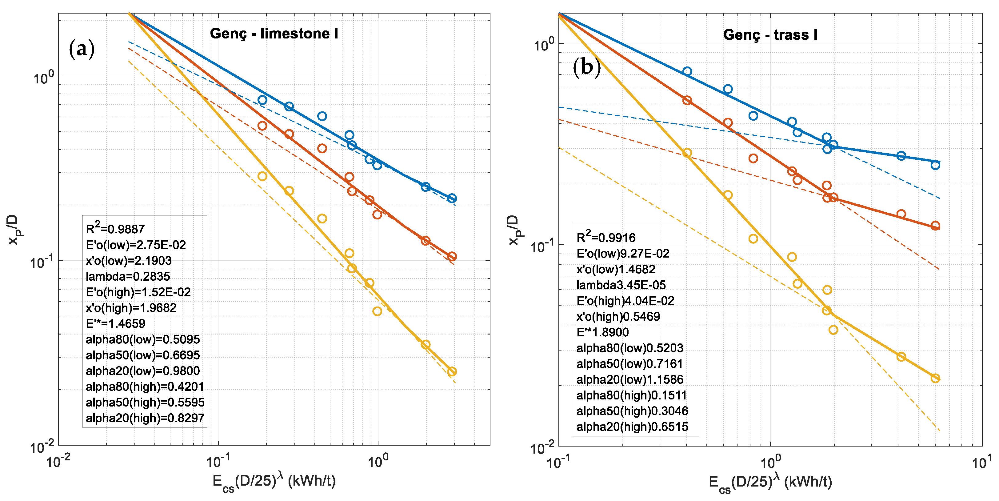
Double fans for Genç’s et al. [24] limestone I (a) and trass I (b). Solid lines are the actual high- and low-energy percentile lines, dashed lines are extrapolations out of their ranges of validity. Circles are data. Percentiles colors: blue—80%, red—50%, yellow—20%.
Figure A3.
Double fans for Genç’s et al. [24] limestone I (a) and trass I (b). Solid lines are the actual high- and low-energy percentile lines, dashed lines are extrapolations out of their ranges of validity. Circles are data. Percentiles colors: blue—80%, red—50%, yellow—20%.

Figure A4.
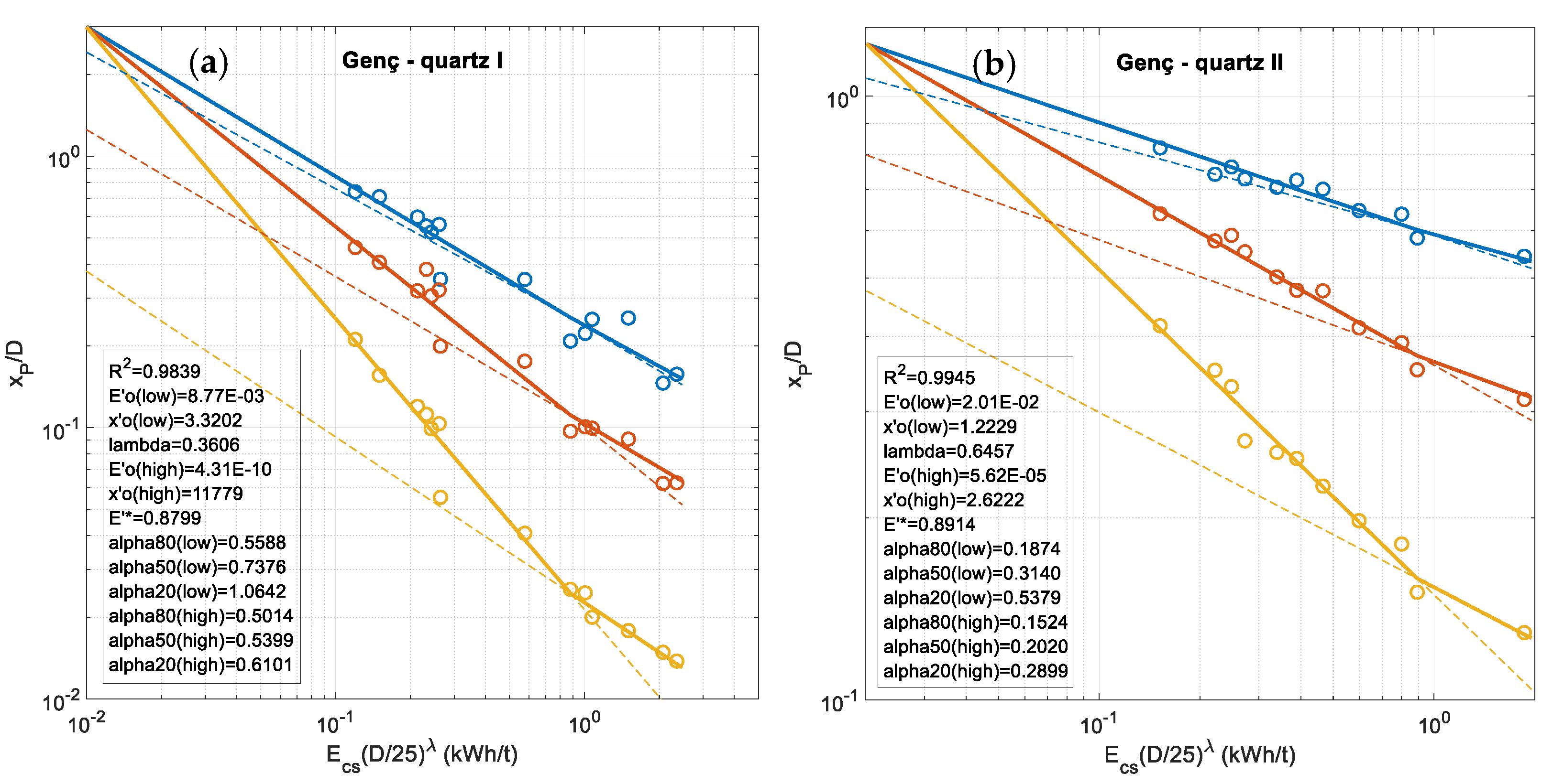
Double fans for Genç’s et al. [24] quartz I (a) and quartz II (b). Solid lines are the actual high- and low-energy percentile lines, dashed lines are extrapolations out of their ranges of validity. Circles are data. Percentiles colors: blue—80%, red—50%, yellow—20%.
Figure A4.
Double fans for Genç’s et al. [24] quartz I (a) and quartz II (b). Solid lines are the actual high- and low-energy percentile lines, dashed lines are extrapolations out of their ranges of validity. Circles are data. Percentiles colors: blue—80%, red—50%, yellow—20%.

Figure A5.
Double fan for Genç’s [25] salt ore (a) and Yu’s [26] Cadia ore (b). Solid lines are the actual high- and low-energy percentile lines, dashed lines are extrapolations out of their ranges of validity. Circles are data. Percentiles colors: blue—80%, red—50%, yellow—20%.

Figure A6.
Double fans for Faramarzi’s [27] ore 1 (a) and ore 2 (b).
Figure A6.
Double fans for Faramarzi’s [27] ore 1 (a) and ore 2 (b).

Figure A7.
Double fans for Faramarzi’s [27] ore 3 (a) and ore 4 (b).
Figure A7.
Double fans for Faramarzi’s [27] ore 3 (a) and ore 4 (b).

Appendix B
Figure A8.
Breakage index plots for Faramarzi’s ore 3 (a,c,e) and Yu’s Cadia ore (b,d,f). (a,b): Banini’s BIE, (c,d): JK new BIE and (e,f): double fan BIE. For both ores, the higher determination is the JK (with in ore 3, = 0.9969, and in Cadia ore, = 0.9365.
Figure A8.
Breakage index plots for Faramarzi’s ore 3 (a,c,e) and Yu’s Cadia ore (b,d,f). (a,b): Banini’s BIE, (c,d): JK new BIE and (e,f): double fan BIE. For both ores, the higher determination is the JK (with in ore 3, = 0.9969, and in Cadia ore, = 0.9365.

Figure A9.
Breakage index plots for (a,c,e) Avsar’s trass and (b,d,f) Avsar’s clinker. (a,b): Banini’s BIE, (c,d): JK new BIE and (e,f) double fan BIE. For trass, the higher determination is Banini’s (= 0.9809); for clinker, it is JK (with , = 0.9941).
Figure A9.
Breakage index plots for (a,c,e) Avsar’s trass and (b,d,f) Avsar’s clinker. (a,b): Banini’s BIE, (c,d): JK new BIE and (e,f) double fan BIE. For trass, the higher determination is Banini’s (= 0.9809); for clinker, it is JK (with , = 0.9941).

Appendix C
Figure A10.
Assessment of the model replication of the raw size distribution data. (a,c,e) basic double fan fit. (b,d,f) direct Swebrec fit. (a,b) Faramarzi’s [27] ore 1; (c,d) Avsar’s [23] clinker (for clarity, only half of the curves have been plotted) and (e,f) Yu’s [26] Cadia ore (for clarity, only a quarter of the curves have been plotted).

Appendix D
Figure A11.
3D breakage plots for Faramarzi’s [27] ore 1. (a) from data. (b) from double fan model (direct fit, constant , ).
Figure A11.
3D breakage plots for Faramarzi’s [27] ore 1. (a) from data. (b) from double fan model (direct fit, constant , ).

Figure A12.
3D breakage plots for Avsar’s [23] clinker. (a) from data. (b) from double fan model (direct fit, variable ).
Figure A12.
3D breakage plots for Avsar’s [23] clinker. (a) from data. (b) from double fan model (direct fit, variable ).

Figure A13.
3D breakage plots for Yu’s [26] Cadia ore. (a) from data. (b) from double fan model (direct fit, variable ).
Figure A13.
3D breakage plots for Yu’s [26] Cadia ore. (a) from data. (b) from double fan model (direct fit, variable ).

References
- Rosin, P.; Rammler, E. The laws governing fineness of powdered coal. J. Inst. Fuel 1933, 7, 29–36. [Google Scholar]
- Cunningham, C.V.B. The Kuz-Ram model for prediction of fragmentation from blasting. In Proceedings of the 1st International Symposium on Rock Fragmentation by Blasting, Luleå University of Technology, Luleå, Sweden, 22–26 August 1983; pp. 439–453. [Google Scholar]
- Cunningham, C.V.B. Fragmentation estimations and the Kuz-Ram model—Four years on. In Proceedings of the 2nd International Symposium on Rock Fragmentation by Blasting, Keystone, CO, USA, 23–26 August 1987; pp. 475–487. [Google Scholar]
- Cunningham, C.V.B. The Kuz-Ram fragmentation model—20 years on. In Proceedings of the 3rd European Federation of Explosives Engineers (EFEE), World Conference on Explosives and Blasting, Brighton, UK, 13–16 September 2005; pp. 201–210. [Google Scholar]
- Ouchterlony, F.; Sanchidrián, J.A. A review of development of better prediction equations for blast fragmentation. J. Rock Mech. Geotech. Eng. 2019, 11, 1094–1109. [Google Scholar] [CrossRef]
- Ouchterlony, F. ‘Bend it Like Beckham’ or a Wide-Range Yet Simple Fragment Size Distribution for Blasted and Crushed Rock; Technical Report 78; EU project GRD-2000-25224 ‘Less Fines’; European Commission: Brussels, Belgium, 2003. [Google Scholar]
- Ouchterlony, F. The Swebrec© function, linking fragmentation by blasting and crushing. Min. Technol. 2005, 114, A29–A44. [Google Scholar] [CrossRef] [Green Version]
- Sanchidrián, J.A.; Ouchterlony, F.; Moser, P.; Segarra, P.; López, L.M. Performance of some distributions to describe rock fragmentation data. Int. J. Rock Mech. Min. Sci. 2012, 53, 18–31. [Google Scholar] [CrossRef]
- Sanchidrián, J.A.; Segarra, P.; López, L.M.; Ouchterlony, F.; Moser, P. On the performance of truncated distributions to describe rock fragmentation. In Measurement and Analysis of Blast Fragmentation; Taylor and Francis: London, UK, 2013; pp. 87–96. [Google Scholar]
- Sanchidrián, J.A.; Ouchterlony, F.; Segarra, P.; Moser, P. Size distribution functions for rock fragments. Int. J. Rock Mech. Min. Sci. 2014, 71, 381–394. [Google Scholar] [CrossRef]
- Sanchidrián, J.A. Ranges of validity of some distribution functions for blast-fragmented rock. In Fragblast 11, Proceedings of the 11th International Symposium Rock Fragmentation by Blasting, Sydney, Australia, 24–26 August 2015; AusIMM: Carlton, VIC, Australia, 2015; pp. 741–748. [Google Scholar]
- Sanchidrián, J.A.; Ouchterlony, F. A distribution-free description of fragmentation by blasting based on dimensional analysis. Rock Mech. Rock Eng. 2017, 50, 781–806. [Google Scholar] [CrossRef] [Green Version]
- Ouchterlony, F.; Sanchidrián, J.A.; Moser, P. Percentile fragment size predictions for blasted rock and the fragmentation–energy fan. Rock Mech. Rock Eng. 2017, 50, 751–779. [Google Scholar] [CrossRef] [Green Version]
- Narayanan, S.S. Development of a Laboratory Single Particle Breakage Technique and Its Application to Ball Mill Scale-Up. Ph.D. Thesis, Julius Kruttschnitt Mineral Research Centre, University of Queensland, Indooroopilly, QLD, Australia, 1985. [Google Scholar]
- Narayanan, S.S.; Whiten, W.J. Breakage characteristics of ores for ball mill modelling. Proc. Australas. Inst. Min. Metall. 1983, 286, 31–39. [Google Scholar]
- Leung, K.; Morrison, R.D.; Whiten, W.J. An energy based ore specific model of autogenous and semi-autogenous grinding. In Copper 87; Chilean Institute of Mining Engineers: Viña del Mar, Chile, 1987. [Google Scholar]
- Andersen, J.S. Development of a Cone Crusher Model. Master’s Thesis, University of Queensland (JKMRC), Indooroopilly, QLD, Australia, 1988. [Google Scholar]
- Napier-Munn, T.J.; Morrell, S.; Morrison, R.D.; Kojovic, T. Mineral Comminution Circuits: Their Operation and Optimization; Julius Kruttschnitt Mineral Research Centre: Indoroopilly, QLD, Australia, 1996. [Google Scholar]
- Banini, G.A. An Integrated Description of Rock Breakage in Comminution Machines. Ph.D. Thesis, Julius Kruttschnitt Mineral Research Centre, University of Queensland, Indoroopilly, QLD, Australia, 2002. [Google Scholar]
- Shi, F. A review of the applications of the JK size-dependent breakage model Part 1: Ore and coal breakage characterization. Int. J. Miner. Process. 2016, 155, 118–129. [Google Scholar] [CrossRef] [Green Version]
- Ouchterlony, F.; Sanchidrián, J.A. The fragmentation-energy fan concept and the Swebrec function in modeling drop weight testing. Rock Mech. Rock Eng. 2018, 51, 3129–3156. [Google Scholar] [CrossRef]
- Shi, F.; Kojovic, T. Validation of a model for impact breakage incorporating particle size effect. Int. J. Miner. Process. 2007, 82, 156–163. [Google Scholar] [CrossRef]
- Avsar, C. Breakage Characteristics of Cement Components. Ph.D. Thesis, Department of Mining Engineering, Middle East Tech University, Ankara, Turkey, 2003. [Google Scholar]
- Genç, Ö.; Ergün, L.; Benzer, H. Single particle impact breakage characterization of materials by drop weight testing. Physicochem Prob. Min. Proc. 2004, 38, 241–255. [Google Scholar]
- Genç, Ö.; Muğla Sıtkı Koçman University, Muğla, Turkey. Sieving Data for Salt Ore. Personal Communication. 2019. [Google Scholar]
- Yu, P. A Generic Dynamic Model Structure for Tumbling Mills. Ph.D. Thesis, Sustainable Minerals Institute, University of Queensland, Indoroopilly, QLD, Australia, 2016. [Google Scholar]
- Faramarzi, F. The Measurement of Variability in Ore Competence and Its Impact on Process Performance. Ph.D. Thesis, Sustainable Minerals Institute, University of Queensland, Indoroopilly, QLD, Australia, 2019. [Google Scholar]
- Yu, P.; Xie, W.; Liu, L.X.; Powell, M.S. The development of the wide-range 4D appearance function for breakage characterisation in grinding mills. Miner. Eng. 2017, 110, 1–11. [Google Scholar] [CrossRef]
- Faramarzi, F.; Jokovic, V.; Morrison, R.; Kanchibotla, S.S. Quantifying variability of ore breakage by impact—Implications for SAG mill performance. Miner. Eng. 2018, 127, 81–89. [Google Scholar] [CrossRef]
- Genç, Ö. An Investigation of the Breakage Distribution Functions of Clinker and Additive Materials. Master’s Thesis, Hacettepe University, Mining Engineering Department, Ankara, Turkey, 2002. [Google Scholar]
- Bourgeois, F. Single-Particle Fracture as a Basis for Microscale Modeling of Comminution Processes. Ph.D. Thesis, Department of Metallurgical Engineering, University of Utah, Salt Lake City, UT, USA, 1993. [Google Scholar]
- Lynch, A.J. (Ed.) Comminution Handbook; AusIMM: Carlton VIC, Australia, 2015. [Google Scholar]
- Ouchterlony, F. Fragmentation characterization; the Swebrec function and its use in blast engineering. In Fragblast 9, Proceedings of the 9th International Rock Fragmentation by Blasting, Granada, Spain, 13–17 September 2009; Sanchidrián, J.A., Ed.; Taylor & Francis: London, UK, 2009; pp. 3–22. [Google Scholar]
- Ouchterlony, F.; Moser, P. Lessons from single-hole blasting in mortar, concrete and rocks. In Fragblast 10, Proceedings of the 10th International Symposium Rock Fragmentation by Blasting, New Delhi, India, 26–29 November 2012; Singh, S., Ed.; Taylor & Francis: London, UK, 2013; pp. 3–14. [Google Scholar]
Figure 7.
Swebrec fits. (a) Large particles, high fidelity over whole size range. (b) Medium sized particles, medium fidelity over whole range. (c) Small particles with lower fidelity, note RR-like curve form. (d) Very small particles with high energy input, high fidelity but datum for x < 0.1 mm excluded. (e) Medium sized particles, excluding rapidly decreasing mass passing values in fines range < 0.1 mm, otherwise high fidelity. (f) Same as (e) but very small particles. Grey area on the right of the graphs is where x > , hence the fit does not apply there. Vertical bars on top are residuals. Relating to Equation (1), the parameters in the heading convert as follows: .

Figure 8.
Double fragmentation energy fans for Avsar’s [23] trass (a) and clinker (b), and Genç’s et al. [24] clinker I (c) and clinker II (d). Circles are data points. Colors correspond to percentage passing: blue 80%, red 50%, yellow 20%.

Figure 9.
Breakage index plots for clinker II (a,c,e) and limestone I (b,d,f). Banini’s BIE (a,b), JK new BIE for = 0 (c,d) and double fan BIE (e,f). For clinker II, the higher determination is the double fan ( = 0.9387); for limestone I it is Banini’s ( = 0.9846).
Figure 9.
Breakage index plots for clinker II (a,c,e) and limestone I (b,d,f). Banini’s BIE (a,b), JK new BIE for = 0 (c,d) and double fan BIE (e,f). For clinker II, the higher determination is the double fan ( = 0.9387); for limestone I it is Banini’s ( = 0.9846).

Figure 10.
Bar chart on the fidelities of the different BIEs for the available data in Table 5 and Table 6.

Figure 11.
BIEs. (a) trass I, basic double fan ( = 0.9776); (b) trass I, double fan I-2 ( = 0.9802); (c) trass I, double fan I-4 ( = 0.9844); (d) Cadia ore double fan I-2 ( = 0.9382), BIE for basic double fan may be seen in Appendix B ( = 0.9313); (e) clinker II, double fan I-2 ( = 0.9433); (f) clinker II, double fan I-3 ( = 0.9478), BIE for basic double fan may be seen in Figure 9 ( = 0.9387).

Figure 12.
Basic double fragmentation-energy fan for Cadia ore (a) and corresponding BIE (b), = 0.9313.
Figure 12.
Basic double fragmentation-energy fan for Cadia ore (a) and corresponding BIE (b), = 0.9313.

Figure 13.
Improved double fan (basic fan with I-4) for Cadia ore (a) and corresponding BIE (b), = 0.9719).
Figure 13.
Improved double fan (basic fan with I-4) for Cadia ore (a) and corresponding BIE (b), = 0.9719).

Figure 14.
Assessment of the model replication of the raw size distribution data. (a) basic double fan fit. (b) direct Swebrec fit. Genç’s et al. [24] limestone I.
Figure 14.
Assessment of the model replication of the raw size distribution data. (a) basic double fan fit. (b) direct Swebrec fit. Genç’s et al. [24] limestone I.

Figure 15.
3D breakage plots for Genç’s et al. [24] limestone I. (a) from data. (b) from double fan model (direct fit, constant , ).
Figure 15.
3D breakage plots for Genç’s et al. [24] limestone I. (a) from data. (b) from double fan model (direct fit, constant , ).

Table 1.
Comparison of fitting fidelities of single and double fragmentation-energy fans with JKMRC’s size-dependent breakage model [22] for Banini’s [19] rocks.
| Fitted BIE | Coot-Tha Hornfels | Newcrest Gold Ore | Mt Isa HG Cu Ore | Mt Isa LG Cu Ore | Mt Isa Pb-Zn Ore 1 | Mt Isa Pb-Zn Ore 2 | Broken Hill Pb-Zn | Big Bell Gold Ore |
|---|---|---|---|---|---|---|---|---|
| Linear fan | 0.982 | 0.980 | 0.980 | 0.960 | 0.960 | 0.967 | 0.965 | 0.954 |
| JK new BIE | 0.993 | 0.987 | 0.989 | 0.981 | 0.982 | 0.982 | 0.981 | 0.980 |
| Double fan | 0.992 | 0.984 | 0.983 | 0.983 | 0.988 | 0.993 | 0.960 | 0.946 |
Table 3.
Results of fitting Swebrec function to sieving data.
| Rock Type | Sieving | ||||||
|---|---|---|---|---|---|---|---|
| Curves | Range | Median | >0.995 | Range | Mean | Std Dev | |
| Banini [19] | |||||||
| hornfels | 42 | 0.9977–0.9999 | 0.9995 | 42 | 1.99–3.91 | 2.48 | 0.35 |
| gold ore | 72 | 0.9985–1.0000 | 0.9998 | 72 | 0.75–3.20 | 2.20 | 0.41 |
| HG Cu ore | 61 | 0.9979–1.0000 | 0.9996 | 61 | 1.69–4.56 | 2.31 | 0.42 |
| LG Cu ore | 70 | 0.9978–1.0000 | 0.9997 | 70 | 1.77–3.61 | 2.31 | 0.41 |
| Pb/Zn ore 1 | 70 | 0.9983–1.0000 | 0.9999 | 70 | 1.77–5.48 | 2.46 | 0.64 |
| Pb/Zn ore 2 | 65 | 0.9946–1.0000 | 0.9999 | 64 | 2.00–5.54b | 2.57 | 0.53 |
| Pb/Zn ore | 47 | 0.9905–1.0000 | 0.9976 | 42 | 0.92–5.38 | 2.23 | 1.03 |
| gold ore | 53 | 0.9812–1.0000 | 0.9991 | 39 | 0.91–5.29 | 1.49 | 0.69 |
| Genç et al. [24] | |||||||
| clay | 4 | 0.9916–0.9997 | 0.9973 | 3 | 2.68–3.34 | 2.95 | 0.31 |
| clinker I | 21 | 0.9974–0.9994 | 0.9989 | 21 | 1.62–2.12 | 1.82 | 0.14 |
| clinker II | 9 | 0.9970–0.9995 | 0.9986 | 9 | 1.44–2.16 | 1.69 | 0.26 |
| colemanite | 9 | 0.9933–0.9988 | 0.9980 | 7 | 2.42–3.30 | 2.81 | 0.27 |
| copper ore | 4 | 0.9979–0.9997 | 0.9987 | 4 | 2.56–4.01 | 3.10 | 0.64 |
| gypsuma | 9 | 0.9886–0.9996 | 0.9983 | 7 | 2.66–17.25 | 10.7 | 5.5 |
| limestone I | 9 | 0.9957–0.9997 | 0.9991 | 9 | 2.03–2.81 | 2.39 | 0.26 |
| quartzite I | 14 | 0.9955–0.9994 | 0.9979 | 14 | 2.20–3.83a | 3.05 | 0.41 |
| quartzite II | 11 | 0.9975–0.9997 | 0.9992 | 11 | 1.77–2.87 | 2.34 | 0.38 |
| trass I | 10 | 0.9978–0.9996 | 0.9986 | 10 | 1.66–2.20 | 1.83 | 0.18 |
| salt orec | 5 | 0.9968–0.9989 | 0.9975 | 5 | 3.58–4.34 | 4.11 | 0.36 |
| Faramarzi [27] | |||||||
| ore 1 | 12 | 0.9984–0.9999 | 0.9996 | 12 | 1.82–2.58 | 2.19 | 0.27 |
| ore 2 | 17 | 0.9966–0.9999 | 0.9996 | 17 | 1.80–2.52 | 2.21 | 0.19 |
| ore 2 | 12 | 0.9978–0.9998 | 0.9990 | 12 | 1.49–2.30 | 1.87 | 0.25 |
| ore 4 | 12 | 0.9993–1.0000 | 0.9996 | 12 | 2.19–2.64 | 2.40 | 0.16 |
| Yu [26] | |||||||
| Cadia porphyry ore | 59 | 0.9893–0.9999 | 0.9976 | 49 | 0.89–3.73 | 2.09 | 0.55 |
| Avsar [23] | |||||||
| clinker | 32 | 0.9956–0.9999 | 0.9985 | 32 | 0.96–2.78 | 2.00 | 0.34 |
| trass | 32 | 0.9953–0.9992 | 0.9971 | 32 | 1.74–3.48 | 2.58 | 0.38 |
| Statistics: | <0.995 | ||||||
| Banini | 480 | min: | 0.9971 | 4.2% | mean: | 2.27 | 0.56 |
| New data | 281 | max: | 0.9999 | 7.8% | mean: | 2.27 | 0.31 |
| Total | 761 | median: | 0.9990 | 5.5% | mean: | 2.27 | 0.47 |
Table 4.
Comparison of -values from CDF fitting with Swebrec function and fan fitting.
| Material | Material | Material | ||||||
|---|---|---|---|---|---|---|---|---|
| clinker | 2.12 | 2.00 | copper ore | 2.37 | 3.10 | salt | 4.03 | 4.11 |
| trass | 2.27 | 2.58 | gypsum | 4.30 | 10.7 | ore 1 | 1.83 | 2.19 |
| clay | 2.35 | 2.95 | limestone I | 2.09 | 2.39 | ore 2 | 1.95 | 2.21 |
| clinker I | 1.64 | 1.82 | quartz I | 2.30 | 3.05 | ore 2 | 1.62 | 1.87 |
| cinker II | 1.57 | 1.69 | quartz II | 2.43 | 2.34 | ore 4 | 2.28 | 2.40 |
| colemanite | 2.22 | 2.81 | trass I | 1.70 | 1.83 | Cadia ore | 1.87 | 2.09 |
Table 5.
fitting ranges and fidelities for different breakage index equations. Bold number: highest -value for that material; underlined number: highest if only 0 allowed.
Table 5.
fitting ranges and fidelities for different breakage index equations. Bold number: highest -value for that material; underlined number: highest if only 0 allowed.
| Material | %–% | JK new BIE | JK New BIE | JK New BIE | Banini BIE Equation (7) | Double Fan Const |
|---|---|---|---|---|---|---|
| 3 param. | 4 param. | 4 param. | 3 param. | 9 param. | ||
| Genç et al. [24] | ||||||
| clay | 16.6–50.1 | 0.9963 | 0.9963 | 1.0000 | 0.9939 | 0.9920 |
| clinker I | 16.2–61.3 | 0.9131 | 0.9199 | 0.9199 | 0.8992 | 0.9289 |
| clinker II | 15.7–71.7 | 0.9132 | 0.9132 | 0.9295 | 0.9034 | 0.9387 |
| colemanite | 22.4–64.8 | 0.9310 | 0.9310 | 0.9451 | 0.9341 | 0.9424 |
| copper ore | 35.6–55.4 | 0.5649 | 0.5649 | 0.7258 | 0.7100 | 0.7908 |
| gypsum | 46.0–60.0 | 0.5797 | 0.5797 | 0.7991 | 0.8353 | 0.6459 |
| limestone I | 6.6–48.1 | 0.9783 | 0.9833 | 0.9833 | 0.9846 | 0.9800 |
| quartz I | 11.4–66.0 | 0.9708 | 0.9708 | 0.9742 | 0.9730 | 0.9750 |
| quartz II | 4.8–15.8 | 0.9456 | 0.9456 | 0.9588 | 0.9553 | 0.8903 |
| trass I | 7.3–42.4 | 0.9712 | 0.9836 | 0.9836 | 0.9571 | 0.9776 |
| salt ore b | 25.2–60.8 | 0.9134 | 0.9134 | 0.9998 | 0.9864 | 0.9944 |
| Faramarzi [27] | ||||||
| ore 1 | 4.0–64.7 | 0.9946 | 0.9952 | 0.9952 | 0.9931 | 0.9943 |
| ore 2 | 3.9–58.0 | 0.9919 | 0.9925 | 0.9925 | 0.9923 | 0.9916 |
| ore 3 | 4.4–54.9 | 0.9965 | 0.9965 | 0.9969 | 0.9939 | 0.9943 |
| ore 4 | 14.0–60.5 | 0.9867 | 0.9867 | 0.9960 | 0.9918 | 0.9943 |
| Yu [26] | ||||||
| Cadia ore | 0.2–51.0 | 0.9353 | 0.9365 | 0.9365 | 0.9333 | 0.9313 |
| Avsar [23] | ||||||
| clinker | 4.0–56.9 | 0.9940 | 0.9941 | 0.9941 | 0.9894 | 0.9919 |
| trass | 5.7–65.9 | 0.9689 | 0.9699 | 0.9699 | 0.9809 | 0.9720 |
| Median: | 0.9699 | 0.9704 | 0.9788 | 0.9770 | 0.9763 | |
Note a: Where the unconstrained regression converges to a positive the values given in this column are the same as in the ≥ 0 column. Note b: Separate salt ore data from [25].
Table 6.
Fidelities, and RMSE (for direct fits, I-5) for improved versions of double fan BIE, compared to results for basic BIE in Table 5, calculating in vs. space. Bold number: highest -value for that material.
Table 6.
Fidelities, and RMSE (for direct fits, I-5) for improved versions of double fan BIE, compared to results for basic BIE in Table 5, calculating in vs. space. Bold number: highest -value for that material.
| Material | Max Fidelity Basic BIE | Type of BIE | Double Fan I-1: 3 Lines ≥ 0a | Double Fan I-1: 3 Lines Any | Double Fan I-2: 3 Lines Variable | Double Fan I-3: 5 Lines Variable | Double Fan I-4: 5 Lines Adapted Variable | Double Fan I-5: Direct Fit Const RMSE | Double Fan I-5: Direct Fit Variable RMSE | |
|---|---|---|---|---|---|---|---|---|---|---|
| 10 param | 10 param | 12 param | 12 param | 12 param | 10 param | 12 param | ||||
| clay | 1.0000 | JK E < 0 | 0.9920 | 0.9945 | few data | 0.9942 | 0.9980 | 1.81 | <0 | 1.85 |
| clink. I | 0.9289 | fan | 0.9300 | 0.9308 | 0.9666 | 0.9662 | 0.9659 | 3.34 | >0 | 2.51 |
| clink. II | 0.9387 | fan | 0.9387 | 0.9387 | 0.9433 | 0.9478 | 0.9482 | 4.36 | >0 | 4.16 |
| colema. | 0.9451 | JK E < 0 | 0.9424 | 0.9447 | 0.9433 | 0.9389 | 0.9447 | 3.03 | <0 | 3.23 |
| Cu ore | 0.7908 | fan | 0.7908 | 0.9623 | few data | 0.9901 | 0.9971 | 1.83 | <0 | 1.46 |
| gyps. | 0.8353 | Banini | 0.6459 | 0.6459 | 0.6464 | 0.7097 | 0.8442 | 2.80 | <0 | 2.79 |
| Lime. I | 0.9846 | Banini | 0.9858 | 0.9977 | 0.9807 | 0.9799 | 0.9829 | 1.63 | >0 | 2.06 |
| qrtz. I | 0.9750 | fan | 0.9750 | 0.9779 | 0.9791 | 0.9755 | 0.9748 | 3.32 | <0 | 3.32 |
| qrtz. II | 0.9588 | JK E < 0 | 0.8903 | 0.8903 | 0.8936 | 0.8941 | 0.9842 | 1.28 | <0 | 1.17 |
| trass I | 0.9836 | JK E ≥ 0 | 0.9777 | 0.9777 | 0.9802 | 0.9818 | 0.9844 | 1.93 | >0 | 1.97 |
| salt ore | 0.9998 | JK E < 0 | 0.9944 | 0.9944 | 0.9941 | 0.9939 | 0.9960 | 2.12 | >0 | 2.17 |
| ore 1 | 0.9952 | JK E ≥ 0 | 0.9944 | 0.9991 | 0.9944 | 0.9940 | 0.9972 | 1.40 | <0 | 1.54 |
| ore 2 | 0.9925 | JK E ≥ 0 | 0.9926 | 0.9926 | 0.9917 | 0.9918 | 0.9921 | 1.60 | <0 | 1.56 |
| ore 3 | 0.9969 | JK E < 0 | 0.9945 | 0.9955 | 0.9943 | 0.9941 | 0.9938 | 1.95 | >0 | 2.02 |
| ore 4 | 0.9960 | JK E < 0 | 0.9943 | 0.9945 | 0.9941 | 0.9945 | 0.9950 | 1.15 | <0 | 1.23 |
| Cadia | 0.9365 | JK E ≥ 0 | 0.9326 | 0.9326 | 0.9382 | 0.9397 | 0.9719 | 6.32(5.11 a) | >0 | 5.13(4.15 a) |
| clinker | 0.9941 | JK E ≥ 0 | 0.9919 | 0.9919 | 0.9924 | 0.9918 | 0.9875 | 1.84 | <0 | 1.87 |
| trass | 0.9809 | Banini | 0.9758 | 0.9758 | 0.9918 | 0.9928 | 0.9917 | 2.34 | >0 | 1.75 |
| Median: | 0.9823 | 0.9768 | 0.9778 | 0.9805 | 0.9860 | 0.9860 | 1.94 | 2.00 |
Note a: Data in parenthesis obtained with the 1135 data points claimed by Yu [26].
Table 7.
Mass passing fidelities of the different versions of the double fan (DF) for selected materials, measured as the errors RMSE. Bold numbers refer to examples plotted in Figure 14 and Figure 15, and Appendix C and Appendix D.
Table 7.
Mass passing fidelities of the different versions of the double fan (DF) for selected materials, measured as the errors RMSE. Bold numbers refer to examples plotted in Figure 14 and Figure 15, and Appendix C and Appendix D.
| Material | DF3: Basic, Double Fan, 3 Fan Lines λ Const. | DF3 w. I-1 Emin ≥ 0 | DF3 w. I-1 Any Emin | DF3 w. I-2 λ Variable | DF5 w. I-3 5 Fan Lines λ Variable | DF5 w. I-4 λ Variable P in t10 Range | Direct Fit Double Fan λ Const. Emin ≥ 0 | Direct Fit Double Fan λ Const. Any Emin | Direct Fit Double Fan λ Variable |
|---|---|---|---|---|---|---|---|---|---|
| No. param. | 9 | 10 | 10 | 12 | 12 | 12 | 10 | 10 | 12 |
| Genç’s | |||||||||
| limestone I | 2.23 | 1.78 | 1.59 | 2.20 | 2.20 | 3.05 | 1.63 | 1.37 | 2.06 |
| Faramarzi’s | |||||||||
| ore 1 | 1.81 | 1.81 | 1.62 | 1.80 | 1.83 | 3.05 | 1.51 | 1.40 | 1.54 |
| Avsar’s | |||||||||
| clinker | 2.70 | 2.70* | 2.54 | 2.55 | 2.46 | 4.70 | 2.11* | 1.84 | 1.87 |
| Yu’s | |||||||||
| Cadia ore | 7.56 | 7.76 | 7.76 | 7.27 | 7.80 | 11.63 | 6.32 | 6.32 | 5.13 |
| 1135 data ** | 6.12 | 6.28 | 6.28 | 5.88 | 6.31 | 9.40 | 5.11 | 5.11 | 4.15 |
* No convergence with the restriction Emin ≥ 0. The result of the fit without Emin as variable (equivalent to Emin = 0) is given. ** Italics refer to RMSE using the 1135 data points claimed by Yu.
Publisher’s Note: MDPI stays neutral with regard to jurisdictional claims in published maps and institutional affiliations. |
© 2021 by the authors. Licensee MDPI, Basel, Switzerland. This article is an open access article distributed under the terms and conditions of the Creative Commons Attribution (CC BY) license (https://creativecommons.org/licenses/by/4.0/).
Share and Cite
MDPI and ACS Style
Ouchterlony, F.; Sanchidrián, J.A.; Genç, Ö. Advances on the Fragmentation-Energy Fan Concept and the Swebrec Function in Modeling Drop Weight Testing. Minerals 2021, 11, 1262. https://0-doi-org.brum.beds.ac.uk/10.3390/min11111262
AMA Style
Ouchterlony F, Sanchidrián JA, Genç Ö. Advances on the Fragmentation-Energy Fan Concept and the Swebrec Function in Modeling Drop Weight Testing. Minerals. 2021; 11(11):1262. https://0-doi-org.brum.beds.ac.uk/10.3390/min11111262
Chicago/Turabian StyleOuchterlony, Finn, José A. Sanchidrián, and Ömürden Genç. 2021. "Advances on the Fragmentation-Energy Fan Concept and the Swebrec Function in Modeling Drop Weight Testing" Minerals 11, no. 11: 1262. https://0-doi-org.brum.beds.ac.uk/10.3390/min11111262
Note that from the first issue of 2016, this journal uses article numbers instead of page numbers. See further details here.