
The Spectral Distribution of Random Mixed Graphs
by
 , and
, and
Yue Guan
, 
Bo Cheng
,
Minfeng Chen
,
Meili Liang
*,†,
Jianxi Liu
*,†,
Jinxun Wang
,
Chao Yang
and
Li Zeng
School of Mathematics and Statistics, Guangdong University of Foreign Studies, Guangzhou 510006, China
*
Authors to whom correspondence should be addressed.
†
These authors contributed equally to this work.
Axioms 2022, 11(3), 126; https://0-doi-org.brum.beds.ac.uk/10.3390/axioms11030126
Submission received: 2 February 2022
/
Revised: 8 March 2022
/
Accepted: 9 March 2022
/
Published: 11 March 2022
(This article belongs to the Special Issue Graph Theory with Applications)
Abstract
:In this work, we propose a random mixed graph model that incorporates both the classical Erdős-Rényi’s random graph model and the random oriented graph model. We show that the empirical spectral distribution of converges to the standard semicircle law under some mild condition, and the Monte Carlo simulation highly agrees with our result.
1. Introduction
A mixed graph is a graph with vertex set and edge set , in which some edges may be undirected and some may be directed. In this paper, the Hermitian adjacency matrix is defined in such a way that the digons (i.e., a pair of arcs with the same end vertices but in opposite directions) may be thought of as undirected edges. From this point of view, digraphs are equivalent to the class of mixed graphs we consider here. The underlying graph of a mixed graph G, denoted by , is the undirected graph that keeps all vertices and edges of G and change every arc of G to an undirected edge.
The notion of a mixed graph generalizes the classical approach of orienting either all edges or none. Undirected graphs, oriented graphs and digraphs are special cases of mixed graphs. We denote an edge (no matter it is directed or not) joining two vertices u and v in G by . A subgraph of a mixed graph is called mixed walk, mixed path or mixed cycle if its underlying graph is a walk, path or cycle, respectively. However, by the terms of order, size, number of components, degree of a vertex, and distance, we mean that they are the same as in their underlying graphs. Let W be a mixed walk of a mixed graph G, its underlying graph (the undirected graph spanned by W in G) may contain parallel edges since W may go through an edge or arcs (no matter in which direction) several of times and thus not necessarily simple. If we take the edge set of without multiplicities, this edge set can span a simple undirected graph which we denote it by . For undefined terminology and notation, we refer the reader to [1].
Let be a random mixed graph on the set of vertices in which independently for each pair of vertices (with ), there is an undirected edge with probability p; there is an arc from to (and the reverse arc does not occur) with probability q; there is an arc from to (and the reverse directed edge does not occur) with probability q; and finally there is no any undirected edge or arc between and with probability (with ). It is immediately to see that is a mixed graph. Note that if we set , then the model is the classical Erdős and Rényi’s random graph model, see [2]; if we set , then the model is the random oriented graph model, see [3]; if we set , then is the random mixed graph model in [4]. Since the parameter , it is easy to see that the random mixed graph model in [4] is not a generalization of the classical Erdős and Rényi’s random graph model. Thus, it is natural for us to build a rather generalized random mixed graph model , which incorporates both classical Erdős and Rényi’s random graph model and the random oriented graph model.
Note that our model is different with the Łuczak and Cohen’s three-parameter random digraphs model [5], as their parameters are absolute constants, but the parameters in our model are functions on n, i.e., and . What is more, they use their model for the study of phase transition of a giant strongly connected component. We will use our model for the study of empirical spectral distribution.
For a digraph G, its classical adjacency matrix is a matrix with rows and columns indexed by the vertices of G, such that the -entry of is equal to 1 if there is an arc from u to v and 0 otherwise. Thus, the classical adjacency matrix of a digraph is not necessary to be symmetric or Hermitian, and thus we cannot guarantee all its eigenvalues to be real. This fact makes the study of the spectrum of digraphs or mixed graphs more difficult than that of undirected graphs. Therefore, Liu and Li [6] and Guo and Mohar [7] independently introduced the Hermitian adjacency matrices of mixed graphs or digraphs. In this work, we will make use of this concept to study the spectral distribution of random mixed graphs.
For brevity, asymptotic notation is used under the assumption that . For functions f and g of parameter n, we use the notation: if as .
The Hermitian adjacency matrix of , denoted by (or , for brevity), satisfies that:
- is a Hermitian matrix with for and all diagonal entries ;
- The upper-triangular entries are independently identically distributed (i.i.d.) copies of a random variable , which takes value 1 with probability p, with probability q, with probability q, and 0 with probability ,
where is the imaginary unit with . Note that , and
Let be a sequence of random Hermitian matrices. Suppose that , are the eigenvalues of . The empirical spectral distribution (ESD) of is defined by
where is the cardinality of the set.
The distribution to which the ESD of converges as is called the limiting spectral distribution (LSD) of .
Wigner matrix, denoted by , is an random Hermitian matrix satisfying:
- The upper-triangular entries are i.i.d. complex random variables with zero mean and unit variance;
- The diagonal entries are i.i.d. real random variables, independent of the upper-triangular entries, with zero mean;
- For each positive integer r, .
Let be a sequence of Wigner matrices. Then, Wigner’s Semicircle Law [8] says that, with probability 1, the ESD of converges to the standard semicircle distribution whose density is given by
Before we give our main results and their proofs, we need the following results.
Lemma 1
(See [9] Lemma 2.4). The number of closed mixed walks of length , which went through each of its edge from vertex to vertex once and its reverse from vertex to vertex once and the underlying graph of the closed mixed walk of a tree is .
Lemma 2
Lemma 3
(See [9] Theorem A.43). Let A and B be two Hermitian matrices, then
where for a function , and means the ESD of A.
Lemma 4
(Dini’s theorem, see [10] p. 64). Suppose that the sequence of continuous functions converges to continuous function on pointwisely. If, for any , the sequence is monotone, then converges to uniformly.
The following result is from [11] p. 264, and we give a proof of it in Appendix A.
Lemma 5.
For any distribution function H, if , then
Lemma 6
(Bernstein’s inequality, see [9] p. 21). If are independent random variables with mean zero and uniformly bounded by b, then for any ,
where and .
Lemma 7
(Borel–Cantelli lemma, see [12] Theorem 3.18). Let be a sequence of events in some probability space. If the sum of the probabilities of the is finite, that is , then the probability that infinitely many of them occur is 0, that is,
Remark 1.
As a result of Lemma 7, for any and any sequence of random variables, we have
- If , then
- If , then .
Define
where is the parameter from , , is the all-ones matrix of order n and is the identity matrix of order n. It is easy to check that
- is Hermitian matrix;
- The diagonal entries and the upper-triangular entries are i.i.d. copies of random variable which takes value with probability p, with probability q, with probability q, and with probability .
Note that and the expectation
On one hand, since , it can easily see from (1) that if as , then for every positive integer s as . Then is a sequence of Wigner matrices and hence LSD of is immediate by the Wigner’s Semicircle Law. On the other hands, if as , then for every positive integer as . Then, is not a sequence of Wigner matrices. Thus, if as , the LSD of cannot be directly derived by the Wigner’s Semicircle Law. In fact, if as , then either or .
For the case , we have
For the case , we have
From the discussion above, we have:
Lemma 8.
The sequence of matrices are Wigner’s matrices if and only if .
Now, we arrive at the main results in the following, which say that even when , we still can get the semicircle distribution of LCD of the corresponding sequences of matrices if holds.
Theorem 1.
Let be a sequence of Hermitian adjacency matrices of random mixed graphs with and . If , then with probability 1, the ESD of converges to the standard semicircle distribution with density .
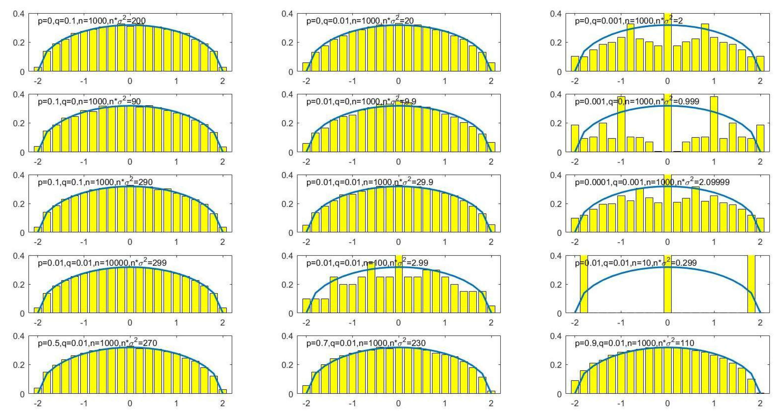
Note that the above result considers an ensemble of random Hermitian matrices, to which the corresponding random mixed graphs are not necessarily connected. Before we proceed to the proof, we use the Monte Carlo method to demonstrate Theorem 1, and it is easy to see from Figure 1 that
- (1)
- As changes from a small value to relatively large value, the ESD becomes more and more close to the semicircle distribution.
- (2)
- In the first row of the Figure 1, we set and changes q increasingly from to (from right to left), then is getting larger and larger, and the ESD is getting more and more close to the semicircle distribution.
- (3)
- In the second row, the similar things happen as the first line except that we fix and change p increasingly from to (from right to left).
- (4)
- In the third row, we fix and increase the values of (from right to left). At this time, we find increases simultaneously with and the ESD is getting more and more close to the semicircle distribution.
- (5)
- In the fourth row, we fix and change n from , 10,000 (from right to left) and at the meantime corresponding increases. Finally, we restore the semicircle law.
- (6)
- In the fifth row we fix and increase the value of p and we find that changes from 110 to 270 (from right to left). All ESDs fit with the semicircle law very well.
Remark 2.
The result of the theorem means that if , then for any bounded continuous function f, we have
Clearly,
Here, is the eigenvalue of the matrix . The proof is exactly the Theorem 1.15 in [13] and we omit it.
Remark 3.
If we set , then our model is the classical Erdős and Rényi’s random graph model. Since if , then . Thus, we could get the result of Theorem 1.3 in [14] as a corollary. Note that the paper [14] is to deal with a much more difficult situation and the original proof of Wigner [8] may be extended without difficulty to derive Theorem 1.3.
Since is equivalent to or . We could say more than that.
Corollary 1
([14]). Let be a sequence of adjacency matrices of random graphs with and . If or , then with probability 1, the ESD of converges to the standard semicircle distribution with density .
Remark 4.
If we set , then our model is essentially the random oriented graph model since the skew-adjacency matrix for an oriented graph G. Therefore, they share the same spectral distribution. Since if , then . Thus, we could get the result of Theorem 3.1 in [3] as a corollary.
Corollary 2
([3]). Let be a sequence of Hermitian adjacency matrices of random oriented graphs with and . If , then with probability 1, the ESD of converges to the standard semicircle distribution with density .
The proof of Theorem 1 will be given in the sequel. We shall first prove the following result.
Theorem 2.
If , then with probability 1, the ESD of converges to the standard semicircle distribution.
Proof.
Denote the r-th moment of the ESD of . Since the standard semicirlular distribution F has finite support, it is uniquely characterized by its sequences of moments. Thus, to prove the weak convergence of to F, it is equivalent to prove the convergence of moments by the Moment Convergence Theorem (see, e.g., [9]), that is
Since
where corresponds to a closed mixed walk of length r in the complete digraph of order n, and is formed by replacing every undirected edge with a pair of arcs in opposite directions in the complete undirected graph of order n. For each edge , let be the number of times that the walk W goes from vertex to vertex . Let . If there is no ambiguity, we will omit the upper symbol for brevity.
Let
Then we rewrite (3) as
Here, the summation is taken over all closed mixed walks W of length r. Note that all different edges (with different pair of end vertices) of a mixed graph are mutually independent, we have
Define , where
Let
and be the r-th moment of the ESD of the matrix . Similar to (3)–(5), we have
and
Next, we will prove that
- Fact 1.
- .
- Fact 2.
- Fact 3.
Combining the above Facts 1–3, we show (2) and complete the proof. □
1.1. Proof of Fact 1
Proof.
The second equality is just the Lemma 2. Now, we consider the remaining equality.
We decompose into parts , containing the m-fold sums,
where
Here, the summation in (9) is taken over all closed mixed walks W of length r with . Additionally, means that the cardinality of the edge set of is m and thus .
For a closed mixed walk . Its underlying graph is connected since there exists an edge between any two vertices and . Note that is a multigraph and is a simple graph. For a closed mixed walks W of length r with , if it goes through some edge only once, then . Hence, if , then there must be some edge that appears only once in W and thus . In the following, we only consider closed mixed walks W of length r with and for all edges in .
If for an edge in . Then,
If for an edge in . Then, by Lemma 5 with and , we have
Moreover, we have
for every edge in with .
Therefore, if we decompose the edge set of into the following set:
then and and we have
Thus, if , we get ; for otherwise
Note that , and then the number of such closed walks W of length r is at most .
Now, we consider the following two cases.
Case 1. The closed walks W of length r with .
We have
Case 2. The closed walks W of length r with .
We then have by the above discussion. We divide this case into two subcases according to the cardinality of .
Subcase 2.1. The closed walks W of length r with .
We have that the number of such closed walks W of length r is at most and
Case 2.2. The closed walks W of length r with and .
We have that for each edge . Since is connected, is a tree with vertices and for every edge . Then, and W is a closed mixed walk of length , which satisfies the condition of Lemma 1. By Lemma 1, the number of such W is . The number of ways to choose vertices of W with the natural order of first appearance in W from n vertices is . Note that and , as . Thus,
Therefore,
From the above discussion, we have
which completes the proof. □
1.2. Proof of Fact 2
Proof.
Note that and since is a real random variable and so is , we have
due to the symmetric of , where corresponds to a closed mixed walk of length r in the complete digraph of order . We aim to show the righthand side in Equation (11) is . Let . If has no any common edge with , where , then the corresponding expectation of the summand in Equation (11) is zero. If there is an edge whose number of occurrence in is 1, then the corresponding expectation of the summand in Equation (11) is also zero. Thus, we only have to consider the case when no edge with and each must share at least one edge with for below. Thus,
For closed mixed walks of length r, let , then and
which implies
Thus,
Similarly, we have
and
Therefore,
Since is a closed mixed walk of length r, is connected. Combining the previous discussions, the connected components of is at most 2. Then, there are at most vertices in , which means that the number of such is at most with a constant only depending on x and r. Hence,
Thus, for every positive integer r
By Lemma 7, we have This finishes the proof of Fact 2. □
1.3. Proof of Fact 3
Proof.
Note that
and
So we have
Notice that the number of nonzero entries in , which is bounded by , where
Then
Note that , we get
Here, the summation occurs among terms. We can show the convergence to zero in the righthand side almost surely using Lemma 6. In fact, set , and for any , we consider
Here, we have used and . Note that
Claim. If , then
If s be any integer no less than 3, then by the Markov’s inequality
By direct calculation, we get that each of the last three summands in (12) tends to zero if .
By the claim above if , we can limit it less than and then we have
Finally we get
which completes the proof by Lemma 7. □
2. Proof of Theorem 1
Proof.
Recall that
and set
Then
By Lemma 3, we have
This implies that and have the same LSD. By Theorem 2, we have
Set . Note that
and
Since , we have that is an eigenvalue of if and only if is an eigenvalue of . By the definition of , we know
Note that by Lemma 4 and the continuity of , we have
Finally we get
This completes the proof. □
3. Conclusions
In this work, we propose a random mixed graph model . The model generalizes the classical Erdős-Rényi’s random graph model and the random oriented graph model. Furthermore, we give a sufficient condition, i.e., if , then with probability 1, the ESD of converges to the standard semicircle distribution. The simulation result not only supports our theorem, but also indicates that the condition may be necessary. We would like to resolve this problem in future work.
Author Contributions
Conceptualization, J.L. and B.C.; methodology, J.L. and Y.G.; software, Y.G.; validation, M.L., M.C. and L.Z.; formal analysis and investigation, J.L., Y.G. and C.Y.; resources, M.L., J.L. and J.W.; writing—original draft preparation, J.L. and Y.G.; writing—review and editing, M.L. and B.C.; supervision, J.L.; project administration, J.L.; funding acquisition, J.L., Y.G., M.C. and M.L. All authors have read and agreed to the published version of the manuscript.
Funding
This research was funded by National Natural Science Foundation of China(No.11701105, No.12001117, No.12001118), Natural Science Foundation of Guangdong Province(No.2016A030313686, No.2018A030313267).
Institutional Review Board Statement
Not applicable.
Informed Consent Statement
Not applicable.
Data Availability Statement
Not applicable.
Acknowledgments
The research was also funded by the Innovation Team Project: “Graph Theory, Cybernetics and Their Applications in Finance” of Guangdong University of Foreign Studies. We would like to thank the anonymous reviewers for their careful work and constructive suggestions that have helped improve this paper substantially.
Conflicts of Interest
The authors declare no conflict of interest.
Appendix A
Lemma A1.
For , if , then .
Proof.
and converges to zero almost surely, by the dominated convergence theorem, we have tends to zero. □
The following result is from [15] with .
Lemma A2.
Suppose as . For , if , then
Proof of Lemma 5.
Suppose that H is the distribution of random variable X. Taking by Lemma A1 we have
Taking , by Lemma A2, we have that , which yields that if . Here we shall take and then since . Meanwhile, , i.e.,
Finally we get
□
References
- Cvetković, D.; Doob, M.; Sachs, H. Spectra of Graphs, 3rd ed.; Johann Ambrosius Barth: Heidelberg, Germany, 1995. [Google Scholar]
- Bollobás, B. Random Graphs; Number 73; Cambridge University Press: Cambridge, UK, 2001. [Google Scholar]
- Chen, X.; Li, X.; Lian, H. The skew energy of random oriented graphs. Linear Algebra Appl. 2013, 438, 4547–4556. [Google Scholar] [CrossRef]
- Hu, D.; Li, X.; Liu, X.; Zhang, S. The spectral distribution of random mixed graphs. Linear Algebra Appl. 2017, 519, 343–365. [Google Scholar] [CrossRef]
- Łuczak, T.; Cohen, J.E. Giant components in three-parameter random directed graphs. Adv. Appl. Probab. 1992, 24, 845–857. [Google Scholar] [CrossRef] [Green Version]
- Liu, J.; Li, X. Hermitian-adjacency matrices and hermitian energies of mixed graphs. Linear Algebra Appl. 2015, 466, 182–207. [Google Scholar] [CrossRef]
- Guo, K.; Mohar, B. Hermitian adjacency matrix of digraphs and mixed graphs. J. Graph Theory 2017, 85, 217–248. [Google Scholar] [CrossRef] [Green Version]
- Wigner, E.P. Characteristic vectors of bordered matrices with infinite dimensions. Ann. Math. 1955, 62, 548–564. [Google Scholar] [CrossRef]
- Bai, Z.; Silverstein, J.W. Spectral Analysis of Large Dimensional Random Matrices; Springer: Berlin/Heidelberg, Germany, 2010; Volume 20. [Google Scholar]
- Royden, H.; Fitzpatrick, P. Real Analysis; Macmillan: New York, NY, USA, 1988; Volume 32. [Google Scholar]
- Arnold, L. On the asymptotic distribution of the eigenvalues of random matrices. J. Math. Anal. Appl. 1967, 20, 262–268. [Google Scholar] [CrossRef] [Green Version]
- Kallenberg, O. Foundations of Modern Probability; Springer Science & Business Media: Berlin/Heidelberg, Germany, 2006. [Google Scholar]
- Guionnet, A. Large random matrices: Lectures on macroscopic asymptotics. In Lecture Notes in Mathematics; Lectures from the 36th Probability Summer School held in Saint-Flour, 2006; Springer: Berlin/Heidelberg, Germany, 2009; Volume 1957. [Google Scholar]
- Tran, L.; Vu, V.; Wang, K. Sparse random graphs: Eigenvalues and eigenvectors. Random Struct. Algorithms 2013, 42, 110–134. [Google Scholar] [CrossRef] [Green Version]
- Heyde, C.; Rohatgi, V. A pair of complementary theorems on convergence rates in the law of large numbers. In Mathematical Proceedings of the Cambridge Philosophical Society; Cambridge University Press: Cambridge, UK, 1967; Volume 63, pp. 73–82. [Google Scholar]
Figure 1.
Simulation for Theorem 1.

Publisher’s Note: MDPI stays neutral with regard to jurisdictional claims in published maps and institutional affiliations. |
© 2022 by the authors. Licensee MDPI, Basel, Switzerland. This article is an open access article distributed under the terms and conditions of the Creative Commons Attribution (CC BY) license (https://creativecommons.org/licenses/by/4.0/).
Share and Cite
MDPI and ACS Style
Guan, Y.; Cheng, B.; Chen, M.; Liang, M.; Liu, J.; Wang, J.; Yang, C.; Zeng, L. The Spectral Distribution of Random Mixed Graphs. Axioms 2022, 11, 126. https://0-doi-org.brum.beds.ac.uk/10.3390/axioms11030126
AMA Style
Guan Y, Cheng B, Chen M, Liang M, Liu J, Wang J, Yang C, Zeng L. The Spectral Distribution of Random Mixed Graphs. Axioms. 2022; 11(3):126. https://0-doi-org.brum.beds.ac.uk/10.3390/axioms11030126
Chicago/Turabian StyleGuan, Yue, Bo Cheng, Minfeng Chen, Meili Liang, Jianxi Liu, Jinxun Wang, Chao Yang, and Li Zeng. 2022. "The Spectral Distribution of Random Mixed Graphs" Axioms 11, no. 3: 126. https://0-doi-org.brum.beds.ac.uk/10.3390/axioms11030126
Note that from the first issue of 2016, this journal uses article numbers instead of page numbers. See further details here.