
Analysis of the Term Structure of Major Currencies Using Principal Component Analysis and Autoencoders


Department of Financial Mathematics, Gachon University, Seongnam 13120, Korea
*
Author to whom correspondence should be addressed.
Axioms 2022, 11(3), 135; https://0-doi-org.brum.beds.ac.uk/10.3390/axioms11030135
Submission received: 5 January 2022
/
Revised: 22 February 2022
/
Accepted: 10 March 2022
/
Published: 15 March 2022
(This article belongs to the Special Issue Mathematical Analysis for Financial Modelling)
Abstract
:Recently, machine-learning algorithms and existing financial data-analysis methods have been actively studied. Although the term structure of government bonds has been well-researched, the majority of studies only analyze the characteristics of one country in detail using one method. In this paper, we analyze the term structure and determine the common factors using principal component analysis (PCA) and an autoencoder (AE). We collected data on the government bonds of three countries with major currencies (the US, the UK, and Japan), extracted features, and compared them. In the PCA-based analysis, we reduced the number of dimensions by converting the normalized data into a covariance matrix and checked the first five principal components visually using graphs. In the AE-based analysis, the model consisted of two encoder layers, one middle layer, and two decoder layers, and the number of nodes in the middle layer was adjusted from one to five. As a result, no significant similarity was found for each country in the dataset, and it was appropriate to extract three features in both methods. Each feature extracted by PCA and the AE had a completely different form, and this appears to be due to the differences in the feature extraction methods. In the case of PCA, the volatility of the datasets affected the features, but in the case of AE, the results seemed to be more affected by the size of the dataset. Based on the findings of this study, this topic can be expanded to compare the results of other machine-learning algorithms or countries.
1. Introduction
The term structure of interest rates occupies a crucial position in the financial field. Term-structure data are used in the pricing of variety bonds and interest rate derivatives (Chacko and Das [1]). Moreover, term structure is very interactive in the establishment of monetary policy (Rudebusch and Wu [2]). Hence, it is an important factor to consider in bond investment strategies. In addition to the bond market, term structure also affects risk management. Treasury bills are used as the basis for establishing a risk-management model related to credit risk and default risk measurement in all national companies (Duffee [3]). Furthermore, the term structure is essential for risk management in a mortgage loan risk model. Because of its importance, many researchers and investors have put a lot of effort into developing and validating term-structure models. For this reason, the term structure is important throughout finance. Therefore, in this study, we analyze the term structure of major currencies using two methods and compare the results.
To analyze term structure, researchers have produced large body of literature that includes a wide variety of models. Nelson and Siegel [4] is famous paper on period structure modeling. The authors assumed that if the model mirrors the standard shape of the term structure instead of approximating it within some tolerance, then it is possible to predict interest rate curves and reasonable prices that deviate from the sample data collected in the study. Their results on US Treasury bill data revealed a high correlation between the current value of a long-term bond indicated by the appropriate curves and the bond’s market price. Subsequently, many studies, e.g., Pooter [5], Koopman et al. [6], Luo et al. [7], and Subramanian [8], have expanded the Nelson–Siegel method for various situations and to include additional factors. Similarly, Svensson [9] expanded the three-factor Nelson–Siegel model to a six-factor model to describe term structure. Christensen et al. [10] uses five different factors (level, two kinds of slope, and curvature) in the Arbitrage-Free Generalized Nelson–Siegel model.
Recently, several studies have attempted to analyze term structure with data-driven models, and principal component analysis (PCA) has been widely used to analyze various term structures (Novosyolov and Satchkov [11], Chantziara and Skiadopoulos [12], Juneja [13], Sowmya et al. [14], Wellmann and Trück [15], Choi [16], Barber [17]). In particular, Novosyolov and Satchkov [11] performed an analysis using PCA on US, EU, and UK Treasury bills, and LIBOR (London Interbank Offered Rate). Furthermore, various machine-learning models such as the multilayer perceptron (MLP), support vector machines, and long short-term memory (LSTM), have been used to analyze term structure (Kanevski et al. [18], Gogas et al. [19], Plakandaras et al. [20], Nunes et al. [21], Suimon et al. [22], Kim et al. [23], Bianchi et al. [24], Jung and Choi [25]). Among the machine-learning approaches, the autoencoder (AE) is a more current method for determining term structure. In fields where multiple factors such as interest rates play a role, dimensionality reduction is a significant issue, and both the accuracy and efficiency of the model should be verified. As with PCA, the AE’s objective is to decrease the number of dimensions of the sample data. A recent study, Kumar [26], compares the results for the three countries (the US, the UK, and Germany) obtained by PCA and an AE. As a result, the research argues that AE is more fitting to the leptokurtic nature of the data. Additional literature on this topic is covered in Section 2.
In this study, we analyzed the term structure of government bond interest rates for the major currencies of the US, UK, and Japan. The goal was to examine the shapes of the features extracted through the AE and PCA and identify the typical differences between them. The reason we adopted these two methods in our study without comparing them with the Nelson–Siegel model is that in several papers, data-driven machine-learning models yielded better analysis or prediction performance than the Nelson–Siegel model (Sambasivan and Das [27], Kim et al. [23]). Furthermore, to create the dataset, we selected treasury bills for the top three currencies (excluding EUR) according to their foreign exchange transaction amounts as of 2021. Transactions in dollars accounted for approximately 88% of all currency exchanges, and the exchanged currency amounts were the highest for EUR, GBP, and JPY, in that order. Therefore, we chose to use the government bond data of the UK, Japan, and the US. Access to each country’s historical data was a secondary reason they were chosen. In each country’s central bank, there should be data related to the interest rate of government bonds with respect to maturity, and a few periods of missing data are likely. In other words, considering the versatility of money, the existence of notarized data is one reason we chose to include each country. The sources of information and datasets for each country’s central bank are described in Section 3.
There are two major aspects of this study that differ from previous studies. First, we compared the features obtained from the term-structure data using the AE model. Few studies analyze term structure using AE, and even fewer studies compare and analyze the AE results. Second, although Kumar [26] focused on comparing the performance of PCA and AE using root-mean-squared error, this study compares the results of each method while controlling the number of extracted features. In addition, we examine the differences in the features extracted by each method intuitively rather than comparing their performance. Unlike this study, the one conducted by Kumar [26] did not set similar conditions to PCA when setting the AE. When the number of encoders and decoders is set to five each for a total of 10, the high predictive power for non-sample data can be seen as a natural result. Thus, this study aims to observe how the shape of each feature is extracted when features are extracted using different methods under similar conditions. Therefore, a follow-up study will be expected to address which methodologies to extract and utilize not only with the interest rate period structure, but also financial data.
The remainder of this paper is organized as follows. Section 2 provides a brief literature review on term structure and studies applying machine-learning algorithms. Section 3 describes the data and methods employed in this study. Section 4 shows the results of empirical analysis for the term structure of major currencies. Finally, we provide concluding remarks in Section 5.
2. Literature Review
There is a vast body of literature on term structure. In this section, we review previous studies by dividing them into studies using the Nelson–Siegel model and studies using machine-learning models.
The Nelson and Siegel [4] yield curve has high utility in models regarding interest rates. Diebold and Li [28] suggested that the Nelson–Siegel method is useful in predicting interest rate term structure. Subsequently, studies were conducted to improve the predictability of interest rates. In a now well-known study, Pooter [5] expanded the three factors used in the Nelson–Siegel model to four factors and improved the predictability of the results. To tune the parameters, Koopman et al. [6] sets the weights of the three factors (level, slope, and curvature), which are expected to be variable with respect to time and then generalizes them, improving out-of-sample prediction results. Christensen et al. [10] added an arbitrage-free condition to analyze the prediction and obtained better results than the existing method, and De Pooter [29] presented the difference between out-of-sample and in-sample prediction by comparing the studies that extended the Nelson–Siegel model. In addition, studies using Nelson–Siegel models that reflect the characteristics of particular countries are as follows. In the case of China, Luo et al. [7] confirmed that the model that increased the weight of the slope among the parameters was most suitable for prediction. Subramanian [8] focused on Indian government bonds, which have low liquidity, for term structure. Considering the differences between countries, Diebold et al. [30] compared the term structures of Germany, Japan, the UK, and the US with their overall statistics. In contrast to research that aims to improve predictability, Goukasian and Cialenco [31] studied how changes in the interest rate term structure are affected by policy.
Furthermore, the use of machine learning in the financial field is being actively pursued. Sambasivan and Das [27] predicted interest rates by maturity using a model trained by machine learning and compared the results with those of the Nelson–Siegel and Gaussian process methods. Research on term-structure analysis based on machine learning has been actively conducted. Bianchi et al. [24] provided statistical evidence in favor of bond return predictability using extreme-tree and neural-network methods. Baruník and Malinska [32] used machine-learning algorithms to predict the term structure of crude oil futures prices, Plakandaras et al. [20] evaluated machine-learning algorithm and econometric methods for predicting US inflation based on the autoregression and structural models of period structures. Gogas et al. [19] used a machine-learning framework to forecast the yield curve in terms of the real gross domestic product (GDP) cycle of the US. Nunes et al. [21] forecasted the European yield curve using two machine-learning techniques: multivariate linear regression and an MLP. Kirczenow et al. [33] applied machine learning to extract features from the historical market-implied corporate bond yields in an illiquid fixed income market. Gogas et al. [19] constructed three models to predict deviations in the real US GDP from its long-term trends over a certain period according to the interest rate and yield curves. In addition, Suimon et al. [22], which is a study that is similar to this paper, analyzed Japanese government bond yields using AE. Kanevski et al. [18] used MLP and support vector machines to extract the features of Swiss franc interest rates. Kim et al. [23] used various machine-learning models (a recurrent neural network (RNN), support vector regression, LSTM, and group method of data handling) to predict credit default swap term structure. Furthermore, they showed that the machine-learning models outperformed the Nelson–Siegel model.
3. Data Description and Methods
3.1. Data Description
We consider the term structure of the currencies of the US, UK, and Japan because they are major currencies. First, there are a total of 3867 data samples from the United States for the period from February 2006 to July 2021. A total of 11 maturities of the US interest rate data were selected: 1 m, 3 m, 6 m, 1y, 2y, 3y, 5y, 7y, 10 y, 20y, and 30y. Next, the UK data were collected from January 2016 to June 2021 and consisted of a total of 1389 data samples. Nine maturities were included: 1y, 2y, 3y, 5y, 7y, 10y, 20y, 25y, and 30y. Finally, in the case of Japan, a total of 4234 samples of interest rate data were collected from March 2004 to June 2021. Fourteen maturities were available, and the data from the 1y to 10y, 15y, 20y, 25y, and 30y maturities were used. We obtained the term structure from each country’s central bank database. The data source for the United States is the daily treasury yield curve rates provided by the US Department of the Treasury. The UK data are yield curves statistics from the Bank of England. In addition, we were able to collect data on Japanese government bonds from the Ministry of Finance.
Table 1 presents the statistics of the term-structure data. The characteristics of the three data sets are briefly summarized as follows. The US Treasury yield spread shows a typical and traditional term structure. It can be observed that the difference between long- and short-term spread rates is the most constant. During the period, the long- to short-term interest spread narrowed as the average interest also rose and then widened again when interest began to decline. Of the three countries, Japan has the most extensive long- to short-term interest spread. The most characteristic part of this dataset is that bills with maturities less than 10 years have negative interest rates on average. Looking at the three datasets, the UK data do not show a lot of change in the spread that is meaningful when the data are visualized. However, the difference between the percentiles is the most significant for all types of maturities, indicating that UK interest rates have fluctuated widely.
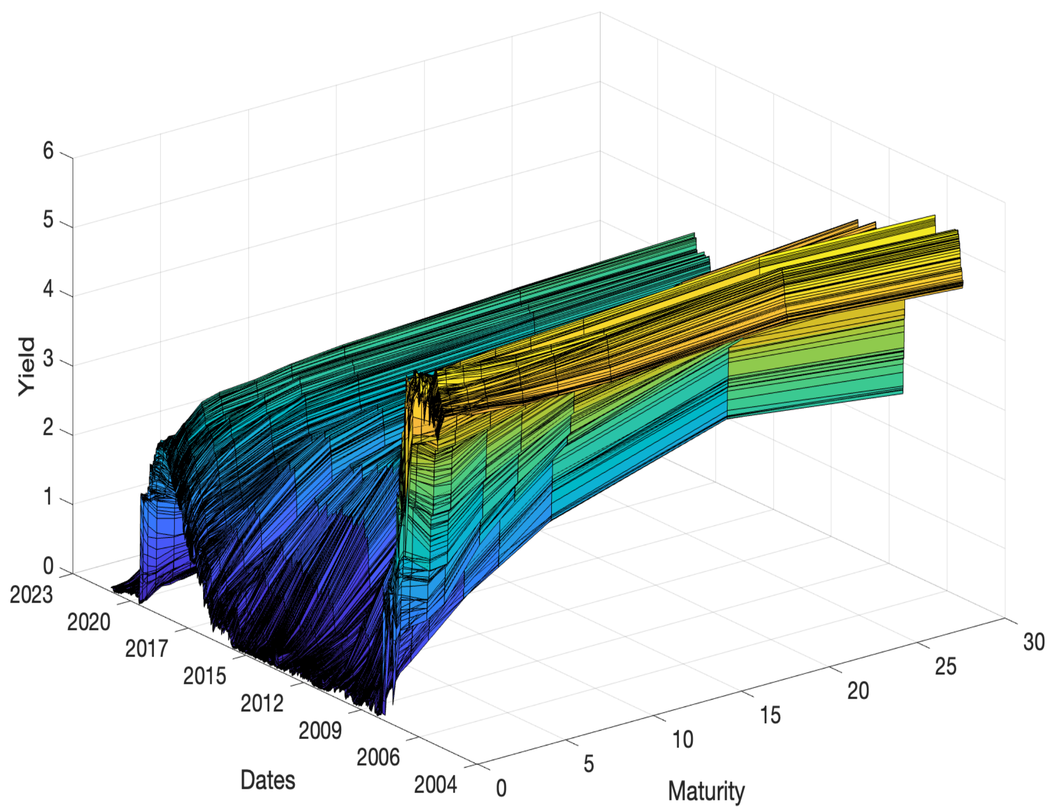
Figure 1 shows the US daily long- to short-term interest rate curves. Each curve represents the state of the curve for one day, and curves for the whole period are given along the third axis. The yellow shades represent interest rates of approximately 5%, and the blue shades represent interest rates of approximately 0.5%. The three-dimensional graph reveals that the interest rates of all government bonds were high at the beginning of the period, but short-term interest rates fell rapidly. Near the end of the period covered by the dataset, long- to short-term interest rates rebounded and then fell again.
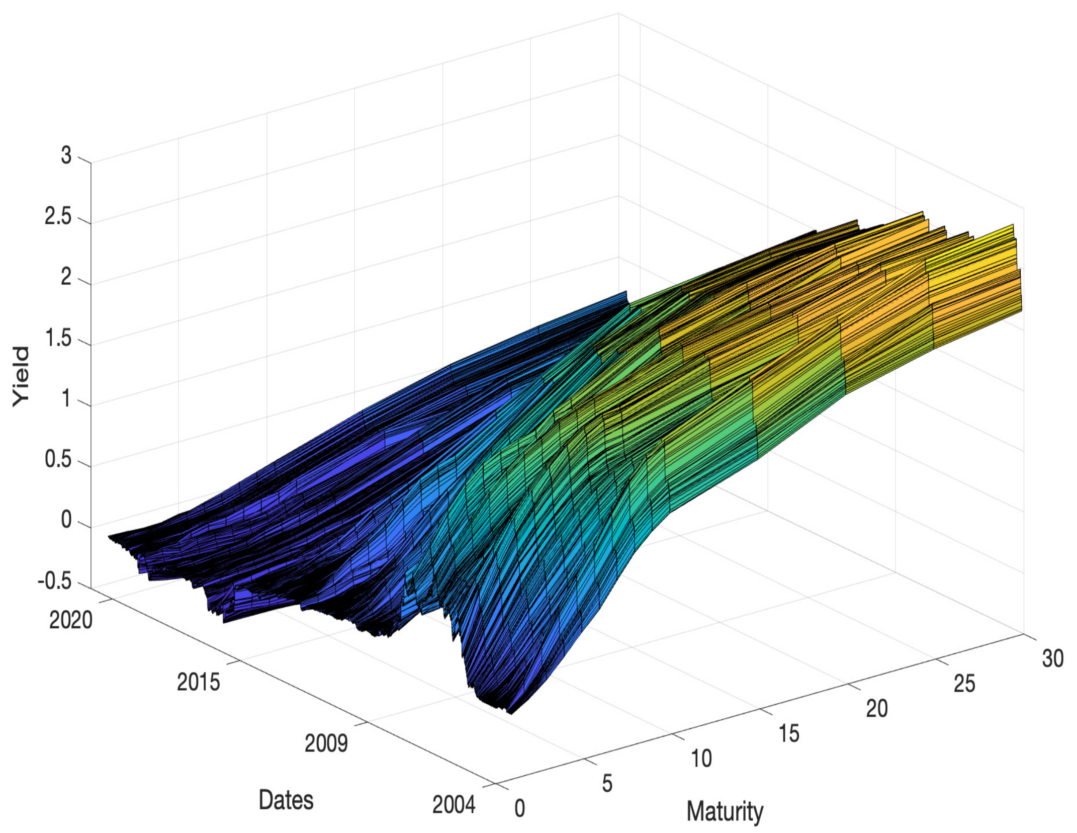
Figure 2 shows these curves for the UK dataset. The number of daily data in this dataset is the smallest of the three datasets, and hence the surface is not dense. One characteristic of these data is that the daily curve has a similar shape, and an overall shallow wave shape can be observed.
Lastly, the Japan data are shown in Figure 3, where the overall curve continuously decreases in height. Of the curves of all three countries, these curves have the flattest overall surface. In contrast to observing the raw data and quantitatively summarizing the dataset, visualizing the data as a three-dimensional graph clearly shows the characteristics of the data of each country.
3.2. PCA
PCA is generally used for dimension reduction or pattern recognition in datasets. In addition, PCA is used to extract the features of a dataset (Cao et al. [34], Ma and Yuan [35]). Therefore, PCA has been widely applied in interest rate markets to describe term structure in terms of several principal components (Litterman and Scheinkman [36], Dai and Singleton [37], Heidari and Wu [38], Novosyolov and Satchkov [11], Blaskowitz and Herwartz [39], Wellmann and Trück [15]).
In this study, we apply PCA to term structure level to extract their best descriptive factors (Dai and Singleton [37], Heidari and Wu [38], Blaskowitz and Herwartz [39], Wellmann and Trück [15]). Generally, PCA can be divided into four steps. The first step standardizes the initial variables; the second computes the covariance matrix; the third computes the eigenvectors and eigenvalues of the covariance matrix; and the fourth creates a feature vector to determine the principal components and validate the PCA results. This procedure can be described mathematically as follows:
Given the original data, and , we standardize it with
where and are the mean and standard deviation, respectively, of the data, .
Let denote the covariance matrix of ; then, it can decompose to , where is a positive diagonal matrix with eigenvalues , where the columns of are the corresponding eigenvectors. Assuming the eigenvectors (principal components) are arranged in decreasing order of eigenvalue, the first K eigenvectors denote the factor loadings, . Then, we obtain the K features, , defined by , where is an N-dimensional vector of the standardized term structure at time t.
To determine how well the principal component explains the data, we use the total variance and the proportion of the m-th principal component given by and , respectively. That is, the proportion is regarded as an explanatory power of each principal component. Accordingly, the principal component with the highest explanatory power becomes the first principal component, and the one with the second highest explanatory power becomes the second, and so on. Finally, the PCA results are visualized as a scree plot. A scree plot is a graph showing the explanatory power of each component in PCA. We refer to several studies (Fengler et al. [40], Novosyolov and Satchkov [11], Barber and Copper [41], Wellmann and Trück [15]) for additional details on PCA mathematical procedures.
3.3. AE
The AE is an artificial neural network trained using an unsupervised learning algorithm. Typical applications of AEs are anomaly detection or noise elimination in image data. In addition, the AE can decrease the number of dimensions of the input data. After Le Cun and Fogelman-Soulié [42] first proposed the concept of the AE, it has been extended to other artificial neural network algorithms. Because of its satisfactory performance, AE is becoming a popular topic; naturally, numerous variations have been introduced by other researchers. The aim of AE is to obtain target values that are equal to the original input values.
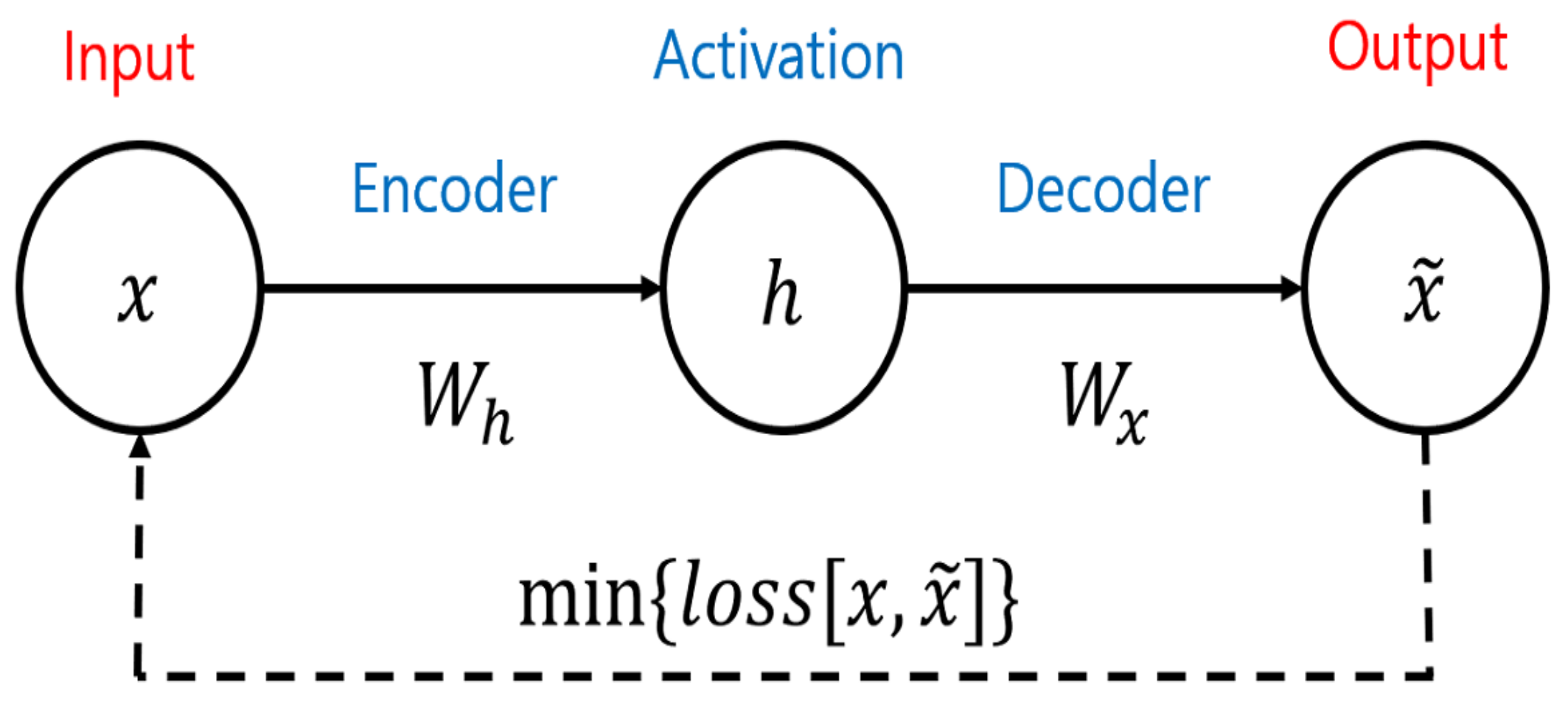
As illustrated in Figure 4, a basic model is usually composed of three phases. The process starts with the encoder, which is defined as an affine transformation after compression. The encoder consists of filters that the model uses to learn essential characteristics of the input and build a hidden layer called h. The decoder is a set of filters that reverses the linear filters and produces a reconstruction of the input data (i.e., through backpropagation). Then, the AE produces an output that is a prediction/reconstruction of the model’s input. We conventionally call this a three-layer neural network, and it can be expressed mathematically by the following equation.
We can observe the visible units x, which are corrupted by b (the bias) and denoted as . is produced in the encoder and denotes the weights between and Similarly, represents the weights in the decoder task. Function h compresses the input data x. For backpropagation, is responsible for using the latent space h and reconstructing input data x. However, the basic form of the AE has a fatal flaw. When the architecture consists of too many hidden layers and units, the amount of calculation can dramatically increase. In addition, the updating value of w decreases, which is called the vanishing gradient. To handle this problem, Bengio et al. [43] introduced the deep belief network and developed the stacked AE. As shown in Figure 5, the output of each previous layer is connected to the input layer to preserve the parameters of the features. The stacked AE inherits the benefits of a deep network, which has greater explanatory power.
4. Results
4.1. PCA
Interest rate data that have been analyzed using PCA are usually interpreted using the three main principal components. This is because the three main principal components (PCs) have the highest explanatory power among all data.
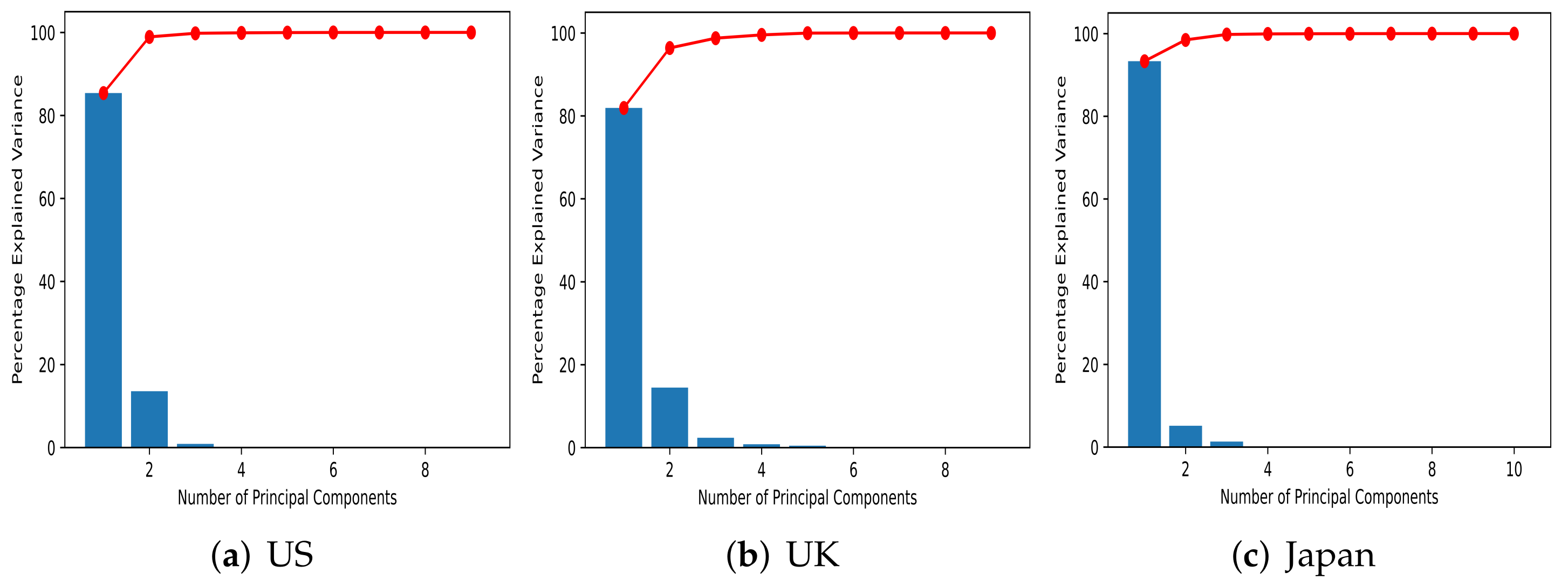
Table 2 shows the explanatory ratios of the components that were obtained when PCA was performed by country on the data. In all three countries, up to the second component (PC 2) represents more than 96% of the information in the data. Among them, the Japanese PC 1 had the highest explanatory power, and the UK PC 1 explained a relatively low proportion of the data. In the case of the US, the first and second components (PC 1 and PC 2) explained 98.91% of the data, and hence they represent most of the dataset. As can be seen from Table 2, seven PCs were extracted for all countries, but only the first three components have significant meaning.
Furthermore, we display the shape of the first three principal components for the three countries in Figure 6. As shown, PC1, PC2, and PC3 indicate level, slope, and curvature, respectively. Similarly, they indicate level, slope, and curvature in the interest rate term structure (Lord and Pelsser [44], Fabozzi et al. [45]).
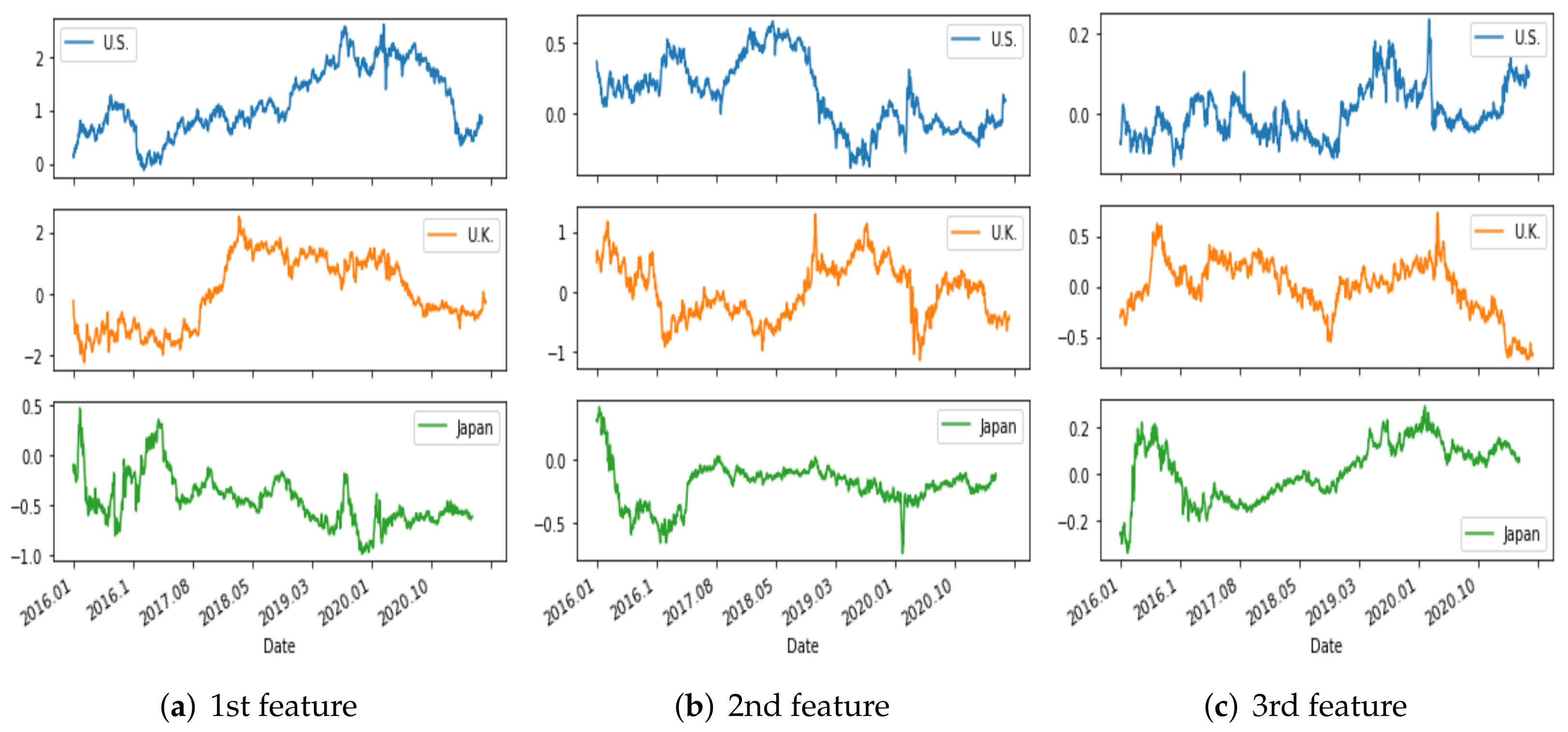
The top three PCs account for 99.78% of the US data. Each feature value time series is shown in Figure 7. For the UK, 98.74% of the data can be explained by three components whose features are shown in Figure 8. Finally, in the case of Japan, the three PCs represent 99.79% of the data, and the features are displayed in Figure 9.
Comparing the features of the three countries over the same period, we observe different aspects of the data. Commonly, feature 1, driven by PC 1, has the most extensive fluctuation of the three factors. The time series of feature 1 for the US, which is initially low, forms a typical yield curve. In contrast, Japan’s feature 1 over a similar sample period has the typical hump shape. Furthermore, Figure 10 compares the results for each country’s feature over the same period, exhibiting completely independent patterns. Thus, these results are appropriate for evaluating other methods. Intuitively, of the three features, feature 1 has the most significant impact on the data. When PC 1 represents the level, it shows a similar pattern as the variation in interest rate. Moreover, Japan’s data tend to follow trends that are opposite those of the other two countries observed in 2016–2020. The results extracted using PCA are generally compared to actual levels, slopes, and curvatures to determine accuracy. However, in this study, the purpose of comparing other methods is to verify model resilience for standard comparison.
The explanatory power examined as a scree plot is shown in Figure 11. Because for all three countries, the first component accounts for 80% or more of the data, the scree plots have an extremely biased shape. In particular, in the case of Japan, because the first component explains 93% of the data, this graph has the most bias. In addition, the third and subsequent components all have a ratio that is difficult to determine from the graph.
4.2. AE
Figure 12, Figure 13 and Figure 14 show the results obtained using the AE. Visually, it can be seen that the features extracted by the AE have greater variability than those obtained using PCA. The activation function used in the AE is tanh, and the structure of the layers is 8-5-3-5-8. Because the interest rate characteristics of each country for PCA were compared using graphs, the seed values used in the encoding and decoding processes of the AE were fixed. When performing time series analysis with an AE, setting the initial weights is also an important issue. In this case, Xavier initialization was judged to be the most appropriate for this time series problem, and hence it was used to set the initial weights for all countries. For the same reason, we set the batch size to one and number of epochs to 50.
In the results obtained for the US data (Figure 12), features 1 and 3 have symmetrical movements, starting from a point where the three features are similar. Moreover, it was confirmed that the symmetrical movement of the two features about one axis is commonly observed with different seed values and for data from other countries.
In the results for the UK data (Figure 13), one feature showed no movement after a rapid change. It is unusual that the features were static in appearance during the period when the interest rate fell and then steadily grew. The results for the Japan data (Figure 14) are generally observed to be more static after large fluctuations than the results for the other two countries. In addition, features 2 and 3 have a symmetrical appearance, as described above.
4.3. Comparisons
4.3.1. Comparison of the PCA and AE Results
The features extracted using PCA are expressed as level, slope, and curvature. In contrast, dimension reduction using an AE does not provide the explanatory power of each feature, and each feature can represent different aspects depending on how the batch size, number of epochs, and activation function are selected. Therefore, it is difficult to compare these methods using guidelines. However, it is interesting to note that compressing three features during the same period yields different results. As a result, it is difficult to consider the three features extracted by AE as the slope, level, and curvature features extracted by PCA, but these features can be seen as compressed features of the entire period.
The features extracted by PCA and the AE for the US data are visually compared in Figure 15. At first glance, it seems that the shape of the graphs are similar for feature 1 of both the AE and PCA results. However, even if the scale is modified and the correlation of each date is considered, the results cannot be considered similar. Comparing feature 1 of PCA with feature 2 of AE using a similar scale, it can be seen that the two curves move in a completely different way.
In the results for the UK data (Figure 16), just looking at the shape of the graphs, it is difficult to determine similarities (as it is for the US results). Some periods in which the shapes of the graphs change abruptly are observed, but similar changes are observed in the samples before 400 and after 1000, although the direction is different. This pattern was observed only in interest rates in the UK, and it is thought that this phenomenon occurs because the size of the dataset for learning and feature extraction is the smallest (approximately 1400 samples). When considered together with the other results, this is meaningful in that some commonalities can be found in the results of AE and PCA depending on the number of data samples.
Finally, comparing the results of the two analyzes for the Japan data (Figure 17), it is also difficult to determine clear commonalities in the graphs. The features extracted through the AE are static and move in one direction. In the Japan data, interest rates have steadily declined and negative interest rates were recorded for a certain period of time, and this may be the reason for the relatively stable results of the AE.
Looking at the graphs of the three countries, it is not easy to determine commonalities, which in general can be seen as a natural result when considering the feature extraction and dimensional compression methods of PCA and AE. Therefore, in this study, to compare various aspects of the methods, the dimensionality reduction of the AE was performed with different settings. We then analyzed the meaning of the AE characteristics by comparing the results of the countries again with the PCA results in a common period.
4.3.2. Comparison of the AE Results Obtained with Different Numbers of Layers
In this study, when three features for the term structure of each country were extracted using an AE, the results differed depending on the activation function, batch size, number of epochs, and initial weight settings.
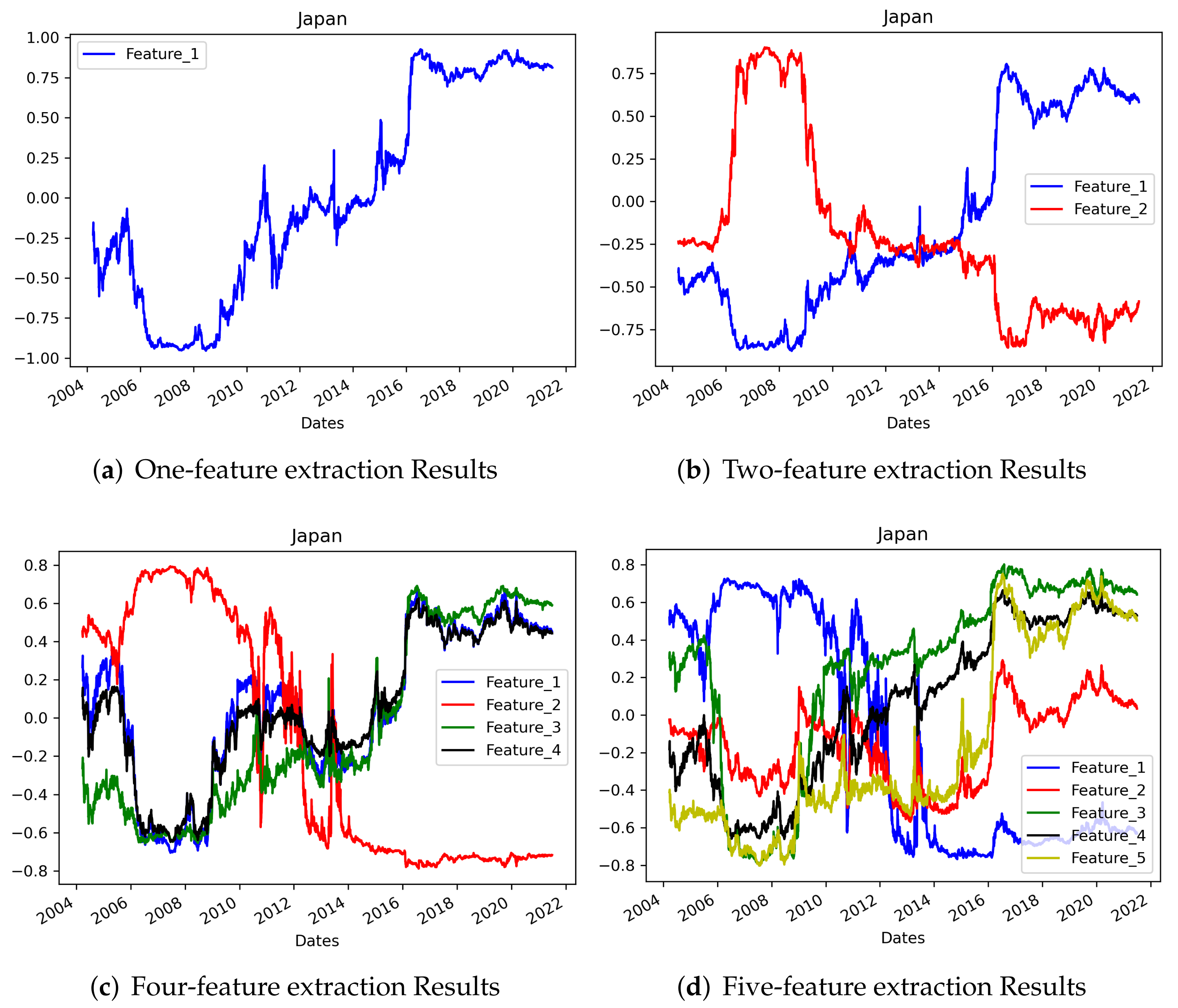
In addition, the number of layers and density seem to be the most important parameter values to set. Hence, we trained term-structure analysis models that extract one to five features. The layers were set the same, but the density of the middle layer was valued from one to five nodes, and the other settings including the seed value were set to the values used for the model that extracts three features. When one to three features were extracted, no common features or singularities in the shape of the graph were observed for each country. However, when four or more features were extracted, overlapping features were observed in three countries. Although the number of overlapping features differed by country, the correlation coefficient between at least two features was at least 0.923 and the highest value was 0.950 (between features 1 and 2 for the US data). This could be observed intuitively in the graphs, as shown in Figure 18, Figure 19 and Figure 20.
One more characteristic of feature extraction at each density setting is that the results obtained when compressed with a low number of feature were included when the results compressed with a higher number of dimensions. For example, looking at each country, the results for the US data when compressed into one dimension had a correlation of 0.942 with the fifth AE feature. The UK data results showed a correlation of 0.992 between the first and third AE features, and the Japan data results showed a correlation of 0.987 between the first and fourth AE features. This result demonstrates that although the order in which the features are extracted from the AE is random, a certain pattern can be observed in the extracted features. In other words, we cannot say that each part of the AE results describe a certain part of the overall term structure like we can for PCA, but there are definitely features that represent the characteristics of the entire term. As the number of extracted features increases, various types of graphs can be drawn, but they are likely to have many overlapping features.
In addition, Table 3 and Table 4 present the correlation coefficients when different numbers of features are extracted in the AE process. Five features were extracted and compared with the results when one to five features were extracted. Table 3 shows the results for one to three features, and a high degree of correlation between the results for five features can be observed throughout the table. In particular, for the UK data, the result when only one feature is extracted and the result when five features are extracted are quite similar. As noted above, the number of samples in the dataset is only 1389, and hence fewer features are observed. Therefore, when the term-structure data are compressed using an AE, more features of the entire period should be observed as the number of samples in the dataset increases. However, it is difficult to see the UK’s relatively stable feature graph form as having the same meaning because the interest rate changes in each country are different. However, a pattern was not found according to the order of features; likewise, a particular form was not seen in each country.
Table 4 shows the results for four and five features, and highly correlated features were inevitably observed. A highly correlated feature was observed even if several features were selected, but from the fourth feature onward, the results reveal a high correlation with the features extracted in the same process. Therefore, when extracting the features of the interest term structure using AE, it seems appropriate to select three features for approximately 4000 samples of data. Observing the entire table, correlation was observed no matter how many features were selected, and this means that the features reflect each other. If too many features are selected, there will be many overlapping features, and if too few features are selected, the overall characteristics will not be represented.
5. Concluding Remarks
In this study, features were extracted using PCA and AE from the term-structure data of government bonds in the US, UK, and Japan, which are countries with major currencies. PCA uses a matrix-based process and compresses the daily interest rate curve to extract the features of the entire period. In the AE, the features of each maturity were learned and extracted through a 8-5-3-5-8 architecture. We set the batch size to one and the number of epochs to 50, and tanh was used as the activation function. To compare the results of each method in more detail, we used the PCA compress the data to one to five dimensions, and one to five features were extracted using the AE.
The three major findings suggested by the results are as follows. First, while extracting features from the interest rate term structure, we observed which features best represent the entire dataset. In the case of PCA, the results seem most appropriate when three features are extracted, regardless of the number of samples in the datasets. The reason is that when the data are compressed into four or more dimensions, the fourth feature appears to overlap with the previous features. In the case of AE, even though each feature had no effect on the explanatory power or order, the features showed a similar shape to previous features when four or more features were extracted. In particular, in most cases, features with high overall correlation coefficients were extracted. When using the AE for analysis, it can be seen that three features are appropriate for datasets with approximately 4000 samples, but the UK data, which consisted of approximately 1300 daily data samples, yielded more overlapping features than did the data of other countries. Therefore, it was found that as the size of the datasets increases, more features can be extracted.
Second, when the similarity of the features extracted through PCA and the AE was intuitively checked, there seems to be no direct correlation. As for the cause of this, in the case of AE, the main reason seems to be that different values are extracted according to the model’s training settings, which include the initial values, activation function, and number of layers. In addition, fundamentally, PCA includes the concept of explanatory power, which represents the entirety of the data in the components, whereas in AE, all features have the same influence. That is, it is difficult to compare features compressed using PCA and features extracted using AE.
Last, looking at each of the results of PCA and AE rather than comparing the two methods, we find the following characteristics. In the case of PCA, even if the correlation coefficient of each characteristic was low, the same movement was observed when the interest rate changed rapidly (even if the direction is different, the form is similar.) In contrast, in the case of the AE, changes in each characteristic were found regardless of the change in the interest rate. This seems to be because the PCA method goes through the process of compression using the covariance matrix of the dataset. In contrast, the AE appears to be less affected by changes in the dataset because the features are predicted and extracted through reconstruction after compression of the dataset.
There are many papers analyzing the interest rate term structure of government bonds through PCA, and it has often been suggested that each feature can be expressed as the level, slope, and curvature of the interest rate. AE is a method commonly used for image, video, and sound processing. There are some instances where it has been applied to time series data, but in relation to this, detailed model tuning and research seem to require a diverse approach, as in this study. Thus, as both PCA and AE methodologies have a common technique of extracting features from data, we found it meaningful to compare their results. In the case of term structure, the results of PCA can be interpreted in terms of level, slope, and curvature. However, AE is an unsupervised learning algorithm used for feature selection in various fields. There are only a few studies that have analyzed features obtained from AE, because there is nothing to which they can be compared. On the contrary, in this study, by comparing the results of PCA and AE for the same term-structure data, we identified the characteristics of the AE-extracted features. Furthermore, the comparison results suggest that further investigation is required to determine the relationship between AE term-structure features, such as orthogonality.
Although an intuitive and clear relationship was not found, it is thought that these results can be a reference for interest rate analysis in future studies. In particular, we note that the results obtained when the number of features extracted is different overlaps with the preceding features’s shape. Method and model composition are also important parts of a study to identify the characteristics of government bonds, but it seems necessary to set the appropriate number of features according to the size of the dataset. If there are more studies applying various methods (e.g., AE, PCA, or the Nelson–Siegel model) to the interest rate sequence and comparing them, improved feature extraction will clearly be possible. In addition, according to the features extracted by PCA and AE, we can investigate the effect of features on the risk management policies for various derivatives related to term structure such as, bonds, credit default swaps, and mortgage loans.
In future studies to analyze interest rate term structure, the following topics are possible. First, the term structures of government bonds of countries other than those used in this study (e.g., Switzerland, Canada, Germany, and Brazil (Tabak [46], Kaminska et al. [47], Wellmann and Trück [15]) may be added. In addition, if cross-country characteristics can be extracted for a common period with sufficiently large datasets (Jorion and Mishkin [48], Sørensen and Werner [49]), it would be possible to better understand the characteristics of the analysis by various methods. Alternatively, even if the datasets are not standardized, it may be meaningful to compare the results of each analysis of the interest rate term structure of major countries such as the G7 countries (Hardouvelis [50]).
Second, the relationship between term structure and exchange rate is interesting and meaningful and should be researched further. Some studies have analyzed the predictive power of term structure for changing exchange rates (Clarida et al. [51], Inci and Lu [52], De Los Rios [53], Bui and Fisher [54], Wellmann and Trück [15]). Accordingly, it will be meaningful to investigate whether the features driven by AE have predictive power with regards to the exchange rate. On the contrary, Kaya [55] showed that the exchange rate provides better forecasting power for term structure. Additionally, by examining US and China yield curves, Hong et al. [56] demonstrated that exchange-rate policy strongly affects changes in term structure. It is also necessary to further investigate how the exchange rate affects features extracted from term structures.
Third, in addition to the methods considered in this paper, there are many other machine-learning algorithms for analyzing time series data. Typically, LSTM and RNN can be used to analyze interest rate curves (Nunes et al. [57], Nunes et al. [58], Ying et al. [59]). The AE model used in this paper is an algorithm of unsupervised learning using a convolutional neural network for classification. The LSTM and RNN architectures can both be used in the AE model. Essentially, the RNN algorithm performs well on ordered data, and LSTM is better for data with structural changes. An AE model based on an RNN may be more accurate than the basic model in that it reflects the information from previous sequence data (Yu et al. [60], Yu et al. [61]). In future research, we will be able to observe the difference in the results by applying these modified and developed algorithms to the same dataset.
Author Contributions
Conceptualization, S.-Y.C.; Methodology, S.C.C. and S.-Y.C.; Software, S.C.C. and S.-Y.C.; formal analysis and investigation, S.C.C. and S.-Y.C.; Writing—original draft, S.C.C.; Writing—review & editing, S.C.C. and S.-Y.C. All authors have read and agreed to the published version of the manuscript.
Funding
The work of S.-Y. Choi was supported by the National Research Foundation of Korea (NRF) grant funded by the Korean government (MSIT) (No. 2021R1F1A1046138) and by the Gachon University research fund of 2021(GCU-202103410001).
Institutional Review Board Statement
Not applicable.
Informed Consent Statement
Not applicable.
Data Availability Statement
The data used to support the findings of this study are available from the corresponding author upon request.
Acknowledgments
We thank the anonymous reviewers; their comments and suggestions helped improve and refine this manuscript.
Conflicts of Interest
The authors declare no conflict of interest.
References
- Chacko, G.; Das, S. Pricing interest rate derivatives: A general approach. Rev. Financ. Stud. 2002, 15, 195–241. [Google Scholar] [CrossRef]
- Rudebusch, G.D.; Wu, T. A macro-finance model of the term structure, monetary policy and the economy. Econ. J. 2008, 118, 906–926. [Google Scholar] [CrossRef] [Green Version]
- Duffee, G.R. The relation between treasury yields and corporate bond yield spreads. J. Financ. 1998, 53, 2225–2241. [Google Scholar] [CrossRef]
- Nelson, C.R.; Siegel, A.F. Parsimonious modeling of yield curves. J. Bus. 1987, 60, 473–489. [Google Scholar] [CrossRef]
- Pooter, M.D. Examining the Nelson-Siegel Class of Term Structure Models; Technical Report, Tinbergen Institute Discussion Paper; SSRN: Rochester, NY, USA, 2007. [Google Scholar]
- Koopman, S.J.; Mallee, M.I.; Van der Wel, M. Analyzing the term structure of interest rates using the dynamic Nelson–Siegel model with time-varying parameters. J. Bus. Econ. Stat. 2010, 28, 329–343. [Google Scholar] [CrossRef] [Green Version]
- Luo, X.; Han, H.; Zhang, J.E. Forecasting the term structure of Chinese Treasury yields. Pac.-Basin Financ. J. 2012, 20, 639–659. [Google Scholar] [CrossRef]
- Subramanian, K. Term structure estimation in illiquid markets. J. Fixed Income 2001, 11, 77–86. [Google Scholar] [CrossRef]
- Svensson, L.E. Estimating and Interpreting Forward Interest Rates: Sweden 1992–1994; National Bureau of Economic Research: Cambridge, MA, USA, 1994. [Google Scholar]
- Christensen, J.H.; Diebold, F.X.; Rudebusch, G.D. An Arbitrage-Free Generalized Nelson–Siegel Term Structure Model; Oxford University Press: Oxford, UK, 2009. [Google Scholar]
- Novosyolov, A.; Satchkov, D. Global term structure modelling using principal component analysis. J. Asset Manag. 2008, 9, 49–60. [Google Scholar] [CrossRef]
- Chantziara, T.; Skiadopoulos, G. Can the dynamics of the term structure of petroleum futures be forecasted? Evidence from major markets. Energy Econ. 2008, 30, 962–985. [Google Scholar] [CrossRef]
- Juneja, J. Common factors, principal components analysis, and the term structure of interest rates. Int. Rev. Financ. Anal. 2012, 24, 48–56. [Google Scholar] [CrossRef]
- Sowmya, S.; Prasanna, K.; Bhaduri, S. Linkages in the term structure of interest rates across sovereign bond markets. Emerg. Mark. Rev. 2016, 27, 118–139. [Google Scholar] [CrossRef]
- Wellmann, D.; Trück, S. Factors of the term structure of sovereign yield spreads. J. Int. Money Financ. 2018, 81, 56–75. [Google Scholar] [CrossRef]
- Choi, S.Y. The influence of shock signals on the change in volatility term structure. Econ. Lett. 2019, 183, 108593. [Google Scholar] [CrossRef]
- Barber, J.R. Empirical analysis of term structure shifts. J. Econ. Financ. 2021, 45, 360–371. [Google Scholar] [CrossRef]
- Kanevski, M.; Maignan, M.; Pozdnoukhov, A.; Timonin, V. Interest rates mapping. Phys. A Stat. Mech. Its Appl. 2008, 387, 3897–3903. [Google Scholar] [CrossRef] [Green Version]
- Gogas, P.; Papadimitriou, T.; Matthaiou, M.; Chrysanthidou, E. Yield curve and recession forecasting in a machine learning framework. Comput. Econ. 2015, 45, 635–645. [Google Scholar] [CrossRef] [Green Version]
- Plakandaras, V.; Gogas, P.; Papadimitriou, T.; Gupta, R. The informational content of the term spread in forecasting the US inflation rate: A nonlinear approach. J. Forecast. 2017, 36, 109–121. [Google Scholar] [CrossRef] [Green Version]
- Nunes, M.; Gerding, E.; McGroarty, F.; Niranjan, M. A comparison of multitask and single task learning with artificial neural networks for yield curve forecasting. Expert Syst. Appl. 2019, 119, 362–375. [Google Scholar] [CrossRef] [Green Version]
- Suimon, Y.; Sakaji, H.; Izumi, K.; Matsushima, H. Autoencoder-based three-factor model for the yield curve of Japanese government bonds and a trading strategy. J. Risk Financ. Manag. 2020, 13, 82. [Google Scholar] [CrossRef]
- Kim, W.J.; Jung, G.; Choi, S.Y. Forecasting Cds term structure based on nelson–siegel model and machine learning. Complexity 2020, 2020, 2518283. [Google Scholar] [CrossRef]
- Bianchi, D.; Büchner, M.; Tamoni, A. Bond risk premiums with machine learning. Rev. Financ. Stud. 2021, 34, 1046–1089. [Google Scholar] [CrossRef]
- Jung, G.; Choi, S.Y. Forecasting Foreign Exchange Volatility Using Deep Learning Autoencoder-LSTM Techniques. Complexity 2021, 2021, 6647534. [Google Scholar] [CrossRef]
- Kumar, R. Towards a Deeper Understanding of Yield Curve Movements. Available at SSRN 3657341. 2020. Available online: https://ssrn.com/abstract=3657341 (accessed on 4 January 2022).
- Sambasivan, R.; Das, S. A statistical machine learning approach to yield curve forecasting. In Proceedings of the 2017 International Conference on Computational Intelligence in Data Science (ICCIDS), Chennai, India, 2–3 June 2017; pp. 1–6. [Google Scholar]
- Diebold, F.X.; Li, C. Forecasting the term structure of government bond yields. J. Econom. 2006, 130, 337–364. [Google Scholar] [CrossRef] [Green Version]
- De Pooter, M. Examining the Nelson-Siegel Class of Term Structure Models: In-sample Fit Versus Out-of-Sample Forecasting Performance. Available at SSRN 992748. 2007. Available online: https://ssrn.com/abstract=992748 (accessed on 4 January 2022).
- Diebold, F.X.; Li, C.; Yue, V.Z. Global yield curve dynamics and interactions: A dynamic Nelson–Siegel approach. J. Econom. 2008, 146, 351–363. [Google Scholar] [CrossRef] [Green Version]
- Goukasian, L.; Cialenco, I. The reaction of term structure of interest rates to monetary policy actions. J. Fixed Income 2006, 16, 76–91. [Google Scholar] [CrossRef]
- Baruník, J.; Malinska, B. Forecasting the term structure of crude oil futures prices with neural networks. Appl. Energy 2016, 164, 366–379. [Google Scholar] [CrossRef] [Green Version]
- Kirczenow, G.; Hashemi, M.; Fathi, A.; Davison, M. Machine Learning for Yield Curve Feature Extraction: Application to Illiquid Corporate Bonds. arXiv 2018, arXiv:1812.01102. [Google Scholar]
- Cao, L.; Chua, K.S.; Chong, W.; Lee, H.; Gu, Q. A comparison of PCA, KPCA and ICA for dimensionality reduction in support vector machine. Neurocomputing 2003, 55, 321–336. [Google Scholar] [CrossRef]
- Ma, J.; Yuan, Y. Dimension reduction of image deep feature using PCA. J. Vis. Commun. Image Represent. 2019, 63, 102578. [Google Scholar] [CrossRef]
- Litterman, R.; Scheinkman, J. Common factors affecting bond returns. J. Fixed Income 1991, 1, 54–61. [Google Scholar] [CrossRef]
- Dai, Q.; Singleton, K.J. Specification analysis of affine term structure models. J. Financ. 2000, 55, 1943–1978. [Google Scholar] [CrossRef]
- Heidari, M.; Wu, L. Are interest rate derivatives spanned by the term structure of interest rates? J. Fixed Income 2003, 13, 75–86. [Google Scholar] [CrossRef]
- Blaskowitz, O.; Herwartz, H. Adaptive forecasting of the EURIBOR swap term structure. J. Forecast. 2009, 28, 575–594. [Google Scholar] [CrossRef] [Green Version]
- Fengler, M.; Härdle, W.; Schmidt, P. Common factors governing VDAX movements and the maximum loss. Financ. Mark. Portf. Manag. 2002, 16, 16. [Google Scholar] [CrossRef] [Green Version]
- Barber, J.R.; Copper, M.L. Principal component analysis of yield curve movements. J. Econ. Financ. 2012, 36, 750–765. [Google Scholar] [CrossRef]
- Le Cun, Y.; Fogelman-Soulié, F. Modèles connexionnistes de l’apprentissage. Intellectica 1987, 2, 114–143. [Google Scholar] [CrossRef]
- Bengio, Y.; Lamblin, P.; Popovici, D.; Larochelle, H. Greedy layer-wise training of deep networks. Adv. Neural Inf. Process. Syst. 2007, 19, 153–160. [Google Scholar]
- Lord, R.; Pelsser, A. Level–Slope–Curvature–Fact or Artefact? Appl. Math. Financ. 2007, 14, 105–130. [Google Scholar] [CrossRef] [Green Version]
- Fabozzi, F.J.; Martellini, L.; Priaulet, P. Predictability in the shape of the term structure of interest rates. J. Fixed Income 2005, 15, 40–53. [Google Scholar] [CrossRef]
- Tabak, B.M. A note on the effects of monetary policy surprises on the Brazilian term structure of interest rates. J. Policy Model. 2004, 26, 283–287. [Google Scholar] [CrossRef]
- Kaminska, I.; Meldrum, A.; Smith, J. A Global Model Of International Yield Curves: No-Arbitrage Term Structure Approach. Int. J. Financ. Econ. 2013, 18, 352–374. [Google Scholar] [CrossRef]
- Jorion, P.; Mishkin, F. A multicountry comparison of term-structure forecasts at long horizons. J. Financ. Econ. 1991, 29, 59–80. [Google Scholar] [CrossRef] [Green Version]
- Sørensen, C.K.; Werner, T. Bank Interest Rate Pass-through in the Euro Area: A cross Country Comparison; Technical Report, ECB Working Paper; European Central Bank: Frankfurt, Germany, 2006. [Google Scholar]
- Hardouvelis, G.A. The term structure spread and future changes in long and short rates in the G7 countries: Is there a puzzle? J. Monet. Econ. 1994, 33, 255–283. [Google Scholar] [CrossRef]
- Clarida, R.H.; Sarno, L.; Taylor, M.P.; Valente, G. The out-of-sample success of term structure models as exchange rate predictors: A step beyond. J. Int. Econ. 2003, 60, 61–83. [Google Scholar] [CrossRef] [Green Version]
- Inci, A.C.; Lu, B. Exchange rates and interest rates: Can term structure models explain currency movements? J. Econ. Dyn. Control 2004, 28, 1595–1624. [Google Scholar] [CrossRef]
- De Los Rios, A.D. Can affine term structure models help us predict exchange rates? J. Ournal Money Credit. Bank. 2009, 41, 755–766. [Google Scholar] [CrossRef]
- Bui, A.T.; Fisher, L.A. The relative term structure and the Australian-US exchange rate. Stud. Econ. Financ. 2016, 33, 417–436. [Google Scholar] [CrossRef]
- Kaya, H. Forecasting the yield curve and the role of macroeconomic information in Turkey. Econ. Model. 2013, 33, 1–7. [Google Scholar] [CrossRef]
- Hong, Z.; Niu, L.; Zeng, G. US and Chinese yield curve responses to RMB exchange rate policy shocks: An analysis with the arbitrage-free Nelson-Siegel term structure model. China Financ. Rev. Int. 2019, 9, 360–385. [Google Scholar] [CrossRef]
- Nunes, M.; Gerding, E.; McGroarty, F.; Niranjan, M. The memory advantage of long short-term memory networks for bond yield forecasting.Available at SSRN 3415219. 2019. Available online: https://ssrn.com/abstract=3415219 (accessed on 4 January 2022).
- Nunes, M.; Gerding, E.; McGroarty, F.; Niranjan, M. Artificial Neural Networks in Fixed Income Markets for Yield Curve Forecasting. Available at SSRN 3144622. 2018. Available online: https://ssrn.com/abstract=3144622 (accessed on 4 January 2022).
- Ying, J.C.; Wang, Y.B.; Chang, C.K.; Chang, C.W.; Chen, Y.H.; Liou, Y.S. DeepBonds: A Deep Learning Approach to Predicting United States Treasury Yield. In Proceedings of the 2019 Twelfth International Conference on Ubi-Media Computing (Ubi-Media), Bali, Indonesia, 5–8 August 2019; pp. 245–250. [Google Scholar]
- Yu, W.; Kim, I.Y.; Mechefske, C. An improved similarity-based prognostic algorithm for RUL estimation using an RNN autoencoder scheme. Reliab. Eng. Syst. Saf. 2020, 199, 106926. [Google Scholar] [CrossRef]
- Yu, W.; Kim, I.Y.; Mechefske, C. Analysis of different RNN autoencoder variants for time series classification and machine prognostics. Mech. Syst. Signal Process. 2021, 149, 107322. [Google Scholar] [CrossRef]
Figure 1.
US term structure.

Figure 2.
UK term structure.

Figure 3.
Japan term structure.

Figure 4.
Basic architecture of the AE.

Figure 5.
Architectures of stacked AEs.

Figure 6.
Representation of the first three principal components.

Figure 7.
Features of US term structure.

Figure 8.
Features of UK term structure.

Figure 9.
Features of Japan term structure.

Figure 10.
Time series of the first three features for the three countries.

Figure 11.
Scree plots.

Figure 12.
US AE prediction result.

Figure 13.
UK AE prediction result.

Figure 14.
Japan AE prediction result.

Figure 15.
Comparison of the results of PCA and AE for the US data.

Figure 16.
Comparison of the results of PCA and AE for the UK data.

Figure 17.
Comparison of the results of PCA and AE for the Japan data.

Figure 18.
AE Results for the US data with different density settings.

Figure 19.
AE Results for the UK data with different density settings.

Figure 20.
AE Results for the Japan data with different density settings.


Table 1.
Statistics for the historical term structure of the three countries. (pctl.: percentile).
| US term structure | |||||||||
| Index | Mean | Std. Dev. | 1st pctl. | 10th pctl. | 25th pctl. | Median | 75th pctl. | 90th pctl. | 99th pctl. |
| 1Y | 1.187 | 0.879 | 0.05 | 0.1 | 0.43 | 1.12 | 1.96 | 2.468 | 2.7 |
| 2Y | 1.294 | 0.873 | 0.11 | 0.15 | 0.54 | 1.3 | 1.96 | 2.56 | 2.88 |
| 3Y | 1.390 | 0.856 | 0.15 | 0.21 | 0.61 | 1.47 | 2.05 | 2.64 | 2.952 |
| 5Y | 1.597 | 0.807 | 0.26 | 0.37 | 0.9 | 1.68 | 2.2 | 2.75 | 3.03 |
| 7Y | 1.805 | 0.756 | 0.44 | 0.582 | 1.31 | 1.84 | 2.35 | 2.828 | 3.111 |
| 10Y | 1.963 | 0.711 | 0.59 | 0.78 | 1.56 | 2 | 2.49 | 2.88 | 3.172 |
| 20Y | 2.297 | 0.596 | 1.01 | 1.302 | 1.92 | 2.33 | 2.78 | 3 | 3.29 |
| 30Y | 2.506 | 0.575 | 1.229 | 1.522 | 2.19 | 2.65 | 2.99 | 3.11 | 3.37 |
| UK term structure | |||||||||
| Index | Mean | Std. Dev. | 1st pctl. | 10th pctl. | 25th pctl. | Median | 75th pctl. | 90th pctl. | 99th pctl. |
| 1Y | 0.314 | 0.297 | −0.124 | −0.033 | 0.049 | 0.245 | 0.562 | 0.747 | 0.862 |
| 2Y | 0.415 | 0.343 | −0.198 | −0.063 | 0.164 | 0.384 | 0.708 | 0.906 | 1.061 |
| 3Y | 0.607 | 0.412 | −0.169 | −0.010 | 0.339 | 0.568 | 0.939 | 1.153 | 1.390 |
| 5Y | 1.018 | 0.536 | 0.052 | 0.195 | 0.539 | 1.135 | 1.466 | 1.644 | 1.983 |
| 7Y | 1.404 | 0.601 | 0.319 | 0.486 | 0.833 | 1.588 | 1.885 | 2.109 | 2.377 |
| 10Y | 1.881 | 0.594 | 0.762 | 0.975 | 1.380 | 2.056 | 2.336 | 2.601 | 2.847 |
| 20Y | 2.076 | 0.557 | 0.935 | 1.285 | 1.663 | 2.157 | 2.424 | 2.610 | 3.364 |
| 30Y | 1.081 | 0.394 | 0.094 | 0.554 | 0.844 | 1.134 | 1.295 | 1.557 | 1.920 |
| Index | Mean | Std. Dev. | 1st pctl. | 10th pctl. | 25th pctl. | Median | 75th pctl. | 90th pctl. | 99th pctl. |
| 1Y | −0.178 | 0.064 | −0.340 | −0.291 | −0.207 | −0.157 | −0.132 | −0.120 | −0.045 |
| 2Y | −0.171 | 0.057 | −0.335 | −0.258 | −0.202 | −0.153 | −0.131 | −0.117 | −0.029 |
| 3Y | −0.163 | 0.061 | −0.351 | −0.250 | −0.191 | −0.149 | −0.124 | −0.101 | −0.014 |
| 5Y | −0.140 | 0.072 | −0.364 | −0.240 | −0.171 | −0.115 | −0.096 | −0.076 | 0.012 |
| 7Y | −0.116 | 0.093 | −0.385 | −0.246 | −0.171 | −0.091 | −0.050 | −0.018 | 0.029 |
| 10Y | 0.007 | 0.093 | −0.273 | −0.127 | −0.043 | 0.031 | 0.063 | 0.099 | 0.220 |
| 20Y | 0.449 | 0.162 | 0.056 | 0.235 | 0.343 | 0.450 | 0.575 | 0.625 | 0.929 |
| 30Y | 0.631 | 0.211 | 0.125 | 0.353 | 0.459 | 0.651 | 0.808 | 0.856 | 1.208 |
Table 2.
Explanatory power of the PCs of the three countries.
| PC’s Explained Proportion | |||||||
|---|---|---|---|---|---|---|---|
| Index | PC1 | PC2 | PC3 | PC4 | PC5 | PC6 | PC7 |
| US | 85.36 | 13.55 | 0.87 | 0.11 | 0.06 | 0.03 | 0.01 |
| U.K. | 81.88 | 14.48 | 2.38 | 0.79 | 0.43 | 0.02 | 0.01 |
| Japan | 93.33 | 5.15 | 1.31 | 0.04 | 0.02 | 0.01 | 0.01 |
Table 3.
Correlation coefficients between the AE results for five features and the AE results for one to three features. Here, N is the number of layers and F.i denotes feature i.
Table 3.
Correlation coefficients between the AE results for five features and the AE results for one to three features. Here, N is the number of layers and F.i denotes feature i.
| Index | F.1 | F.2 | F.3 | F.4 | F.5 | |
| US | F.1 | 0.147 | −0.137 | −0.590 | −0.930 | 0.942 |
| UK | F.1 | 0.896 | −0.972 | 0.992 | −0.914 | 0.900 |
| Japan | F.1 | −0.861 | 0.528 | 0.911 | 0.987 | 0.946 |
| Index | F.1 | F.2 | F.3 | F.4 | F.5 | |
| US | F.1 | 0.967 | 0.853 | 0.328 | −0.095 | 0.368 |
| F.2 | 0.286 | 0.550 | 0.743 | 0.974 | −0.877 | |
| UK | F.1 | 0.829 | 0.934 | 0.987 | −0.935 | 0.901 |
| F.2 | −0.959 | 0.994 | −0.960 | 0.887 | −0.887 | |
| Japan | F.1 | −0.798 | 0.629 | 0.858 | 0.959 | 0.983 |
| F.2 | 0.785 | −0.489 | −0.990 | −0.920 | −0.804 | |
| Index | F.1 | F.2 | F.3 | F.4 | F.5 | |
| US | F.1 | 0.829 | 0.941 | 0.650 | 0.588 | −0.358 |
| F.2 | 0.106 | 0.339 | 0.578 | 0.801 | −0.811 | |
| F.3 | −0.576 | −0.329 | 0.299 | 0.686 | −0.862 | |
| UK | F.1 | 0.890 | −0.969 | 0.994 | −0.919 | 0.898 |
| F.2 | −0.917 | 0.965 | −0.961 | 0.862 | −0.844 | |
| F.3 | 0.657 | −0.815 | 0.896 | −0.977 | 0.979 | |
| Japan | F.1 | 0.617 | −0.760 | −0.698 | −0.834 | −0.979 |
| F.2 | 0.571 | −0.326 | −0.900 | −0.688 | −0.495 | |
| F.3 | −0.894 | 0.469 | 0.926 | 0.996 | 0.921 | |
Table 4.
Correlation coefficients between the AE results for five features and the AE results for four and five features. Here, Here, N is the number of layers and F.i denotes feature i.
Table 4.
Correlation coefficients between the AE results for five features and the AE results for four and five features. Here, Here, N is the number of layers and F.i denotes feature i.
| Index | F.1 | F.2 | F.3 | F.4 | F.5 | |
| US | F.1 | 0.972 | 0.961 | 0.472 | 0.230 | 0.090 |
| F.2 | 0.638 | 0.395 | −0.171 | −0.640 | 0.833 | |
| F.3 | 0.513 | 0.737 | 0.768 | 0.909 | −0.710 | |
| F.4 | 0.848 | 0.659 | 0.194 | −0.355 | 0.594 | |
| UK | F.1 | 0.902 | −0.981 | 0.996 | −0.940 | 0.925 |
| F.2 | −0.696 | 0.515 | −0.336 | 0.064 | −0.058 | |
| F.3 | 0.826 | −0.937 | 0.992 | −0.964 | 0.936 | |
| F.4 | −0.652 | 0.817 | −0.912 | 0.989 | −0.970 | |
| Japan | F.1 | −0.575 | 0.741 | 0.898 | 0.844 | 0.862 |
| F.2 | 0.991 | −0.175 | −0.859 | −0.954 | −0.781 | |
| F.3 | −0.781 | 0.635 | 0.828 | 0.947 | 0.987 | |
| F.4 | −0.704 | 0.684 | 0.931 | 0.924 | 0.920 | |
| Index | F.1 | F.2 | F.3 | F.4 | F.5 | |
| US | F.1 | 1 | 0.951 | 0.612 | 0.637 | −0.911 |
| F.2 | 1 | 0.507 | 0.423 | −0.570 | ||
| F.3 | 1 | −0.730 | −0.866 | |||
| F.4 | 1 | 0.153 | ||||
| F.5 | 1 | |||||
| UK | F.1 | 1 | −0.966 | −0.967 | −0.943 | −0.990 |
| F.2 | 1 | 0.876 | 0.873 | 0.923 | ||
| F.3 | 1 | −0.730 | −0.866 | |||
| F.4 | 1 | 0.726 | ||||
| F.5 | 1 | |||||
| Japan | F.1 | 1 | 0.043 | 0.356 | 0.926 | 0.890 |
| F.2 | 1 | −0.803 | 0.344 | 0.762 | ||
| F.3 | 1 | −0.914 | 0.677 | |||
| F.4 | 1 | −0.685 | ||||
| F.5 | 1 | |||||
Publisher’s Note: MDPI stays neutral with regard to jurisdictional claims in published maps and institutional affiliations. |
© 2022 by the authors. Licensee MDPI, Basel, Switzerland. This article is an open access article distributed under the terms and conditions of the Creative Commons Attribution (CC BY) license (https://creativecommons.org/licenses/by/4.0/).
Share and Cite
MDPI and ACS Style
Chae, S.C.; Choi, S.-Y. Analysis of the Term Structure of Major Currencies Using Principal Component Analysis and Autoencoders. Axioms 2022, 11, 135. https://0-doi-org.brum.beds.ac.uk/10.3390/axioms11030135
AMA Style
Chae SC, Choi S-Y. Analysis of the Term Structure of Major Currencies Using Principal Component Analysis and Autoencoders. Axioms. 2022; 11(3):135. https://0-doi-org.brum.beds.ac.uk/10.3390/axioms11030135
Chicago/Turabian StyleChae, Soo Chang, and Sun-Yong Choi. 2022. "Analysis of the Term Structure of Major Currencies Using Principal Component Analysis and Autoencoders" Axioms 11, no. 3: 135. https://0-doi-org.brum.beds.ac.uk/10.3390/axioms11030135
Note that from the first issue of 2016, this journal uses article numbers instead of page numbers. See further details here.