On the Laplacian, the Kirchhoff Index, and the Number of Spanning Trees of the Linear Pentagonal Derivation Chain

Abstract

Let $P_n$ be a pentagonal chain with $2n$ pentagons in which two pentagons with two edges in common can be regarded as adding one vertex and two edges to a hexagon. Thus, the linear pentagonal derivation chains $Q{P}_n$ represent the graph obtained by attaching four-membered rings to every two pentagons of $P_n$. In this article, the Laplacian spectrum of $Q{P}_n$ consisting of the eigenvalues of two symmetric matrices is determined. Next, the formulas for two graph invariants that can be represented by the Laplacian spectrum, namely, the Kirchhoff index and the number of spanning trees, are studied. Surprisingly, the Kirchhoff index is almost one half of the Wiener index of a linear pentagonal derivation chain $Q{P}_n$.

1. Introduction

In this work, we will use terminologies and traditional notations from [1]. Let $G=\left(V\right(G),E(G\left)\right)$ be a finite, simple, and undirected connected graph with vertex set $V\left(G\right)=\{v_1,v_2,\cdots ,v_n\}$ and edge set $E\left(G\right)$. The order of G is the number $\left|V\right(G\left)\right|$ of its vertices and its size is the number $\left|E\right(G\left)\right|$ of its edges. The adjacency matrix of G, denoted by $A\left(G\right)$, is a $0-1$ $n\times n$ matrix whose $(i,j)$-entry is equal to 1 if $v_i$ and $v_j$ are adjacent in G and 0 otherwise. The degree of $v_i$ in G is denoted by $d_i=d_G\left(v_i\right)$.

The Laplacian matrix of G is the matrix $L\left(G\right)=D\left(G\right)-A\left(G\right)$, where $D\left(G\right)$ is the diagonal matrix of G whose diagonal entries are the degrees of the vertices of G. The characteristic polynomial of $L\left(G\right)$ is defined as

$${\Phi }_{L\left(G\right)}\left(\lambda \right)=det(\lambda I_n-L\left(G\right)),$$

where $I_n$ is the identity matrix of order n. Note that $L\left(G\right)$ is positive semi-definite. The Laplacian spectrum of G is denoted by $spec\left(L\left(G\right)\right)=\{{\mu }_1,{\mu }_2,\cdots ,{\mu }_n\}$, and we assume that the eigenvalues are labeled such that $0={\mu }_1<{\mu }_2\le \cdots \le {\mu }_n$.

The distance between vertices $v_i$ and $v_j$ in G, denoted by $d_{ij}=d(v_i,v_j)$, is the length of the shortest path between them in G. The Wiener index, a distance-based topological index, was first presented by Wiener in chemistry back in 1947 [2] and in mathematics about 40 years later [3]. The famous Wiener index $W\left(G\right)$ is defined as

$$W\left(G\right)=\sum _{i<j}{d}_{ij},$$

where the sum is taken over all distances between pairs of vertices of G.

At present, the Wiener index has been widely studied, and many research results have been obtained [4,5,6,7,8,9].

The topological index in a graph distance function can explain the structure and properties of a graph well. In 1993, Klein and Randić [10] introduced a distance function named resistance distance on the basis of electrical network theory. The resistance distance between vertices $v_i$ and $v_j$, denoted by $r_{ij}$, is defined to be the effective electrical resistance between them if each edge of G is replaced by a unit resistor. One famous resistance distance-based parameter called the Kirchhoff index, $Kf\left(G\right)$ [10], was given by

$$Kf\left(G\right)=\sum _{i<j}{r}_{ij}.$$

Moreover, Klein and Randić [10] proved that $r_{ij}\le d_{ij}$ and $Kf\left(G\right)\le W\left(G\right)$ with equality if and only if G is a tree.

Similar to the Wiener index, the Kirchhoff index is also intrinsic to the graph, not only with some fine, purely mathematical properties, but also with a substantial potential for chemical applications. Unfortunately, it is difficult to compute the resistant distance and Kirchhoff index in a graph due to their computational complexity. Thus, it is necessary to find closed-form formulas for the Kirchhoff index.

It is worth noting that the resistance distance between any two vertices can be obtained in terms of the eigenvalues and eigenvectors of the Laplacian matrix in an electronic network. Therefore, for any connected graph G of order $n\ge 2$, it is shown, independently, by Gutman and Mohar [11] and Zhu et al. [12] that

$$Kf\left(G\right)=\sum _{i<j}{r}_{ij}=n\sum _{i=2}^n\frac{1}{{\mu }_i}.$$

(1)

For some graphs with a good structure, such as graphs with good periodicity and good symmetry, researchers can calculate the closed-form formulas of the Kirchhoff index of those graphs. Readers are referred to the references [13,14,15,16,17,18] and the references therein.

A linear pentagonal chain of length n, denoted by $P_n$, is a pentagonal chain with $2n$ pentagons in which two pentagons with two edges in common can be regarded as adding one vertex and two edges to a hexagon. Wang and Zhang [19] obtained the explicit closed-form formulas of the Kirchhoff index of linear pentagonal chains. Wei et al. [20] made comparisons between the expected values of the Wiener index and the Kirchhoff index in random pentachains and presented the average values of the Wiener and Kirchhoff indices with respect to the set of all random pentachains with n pentagons. Recently, Sahir and Nayeem [21] derived closed-form formulas for the Kirchhoff index and the Wiener index of the linear pentagonal cylinder graph and the linear pentagonal Möbius chain graph. The study of hexagonal systems have attracted interest because they are natural graph representations of benzenoid hydrocarbon [22], and they have been of great interest and extensively studied; see [5,17,23].

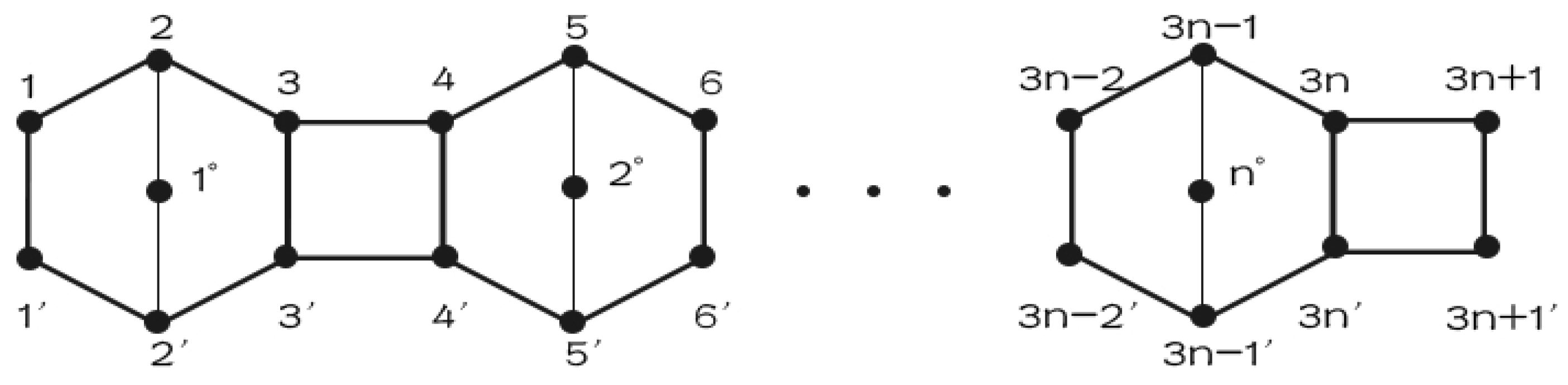
Consider a linear pentagonal chain $P_n$ consisting of $2n$ pentagons. The linear pentagonal derivation chain, denoted by $Q{P}_n$, is thus the graph obtained by attaching four-membered rings to every two pentagons of $P_n$, as depicted in Figure 1. It is easy to check that $\left|V\right(Q{P}_n\left)\right|=7n+2$, $\left|E\right(Q{P}_n\left)\right|=10n+1$. Obviously, the linear pentagonal derivation chain $Q{P}_n$ is different from random pentachains, a linear pentagonal cylinder graph, and a linear pentagonal Möbius chain graph.

In this paper, we focus on the linear pentagonal derivation chain $Q{P}_n$. Firstly, the Laplacian spectrum of $Q{P}_n$ consisting of the eigenvalues of two symmetric matrices, is determined. Next, using the decomposition theorem for the Laplacian characteristic polynomial, the explicit closed-form formulas for the Kirchhoff index and the number of spanning trees of $Q{P}_n$ can be represented. Interestingly, the Kirchhoff index is about half of the Wiener index of a linear pentagonal derivation chain $Q{P}_n$.

2. Laplacian Polynomial Decomposition and Some Preliminary Results

An automorphism of G is a permutation $\pi$ of $V\left(G\right)$, which has the property that $v_i{v}_j$ is an edge of G if and only if $\pi \left(v_i\right)\pi \left(v_j\right)$ is an edge of G. Suppose that G has an automorphism $\pi$. It can then be written as the product of disjoint 1-cycles and transpositions.

Assume we label the vertices of $Q{P}_n$ as in Figure 1 and denote

$$V_0=\{1^{\circ },2^{\circ },\dots ,n^{\circ }\},V_1=\{1,2,\dots ,3n+1\},V_2=\{1^{{}^{\prime }},2^{{}^{\prime }},\dots ,{(3n+1)}^{{}^{\prime }}\}.$$

Therefore,

$$\pi =\left(1^{\circ }\right)\left(2^{\circ }\right)\cdots \left(n^{\circ }\right)(1,1^{{}^{\prime }})(2,2^{{}^{\prime }})\cdots (3n+1,{(3n+1)}^{{}^{\prime }})$$

is an automorphism of $Q{P}_n$. Hence, the Laplacian matrix $L\left(G\right)$ of $Q{P}_n$ can be written as the following block matrix:

$$L\left(G\right)=\begin{array}{c}\left[\begin{array}{ccc}{L}_{V_0{V}_0}& L_{V_0{V}_1}& L_{V_0{V}_2}\\ L_{V_1{V}_0}& L_{V_1{V}_1}& L_{V_1{V}_2}\\ L_{V_2{V}_0}& L_{V_2{V}_1}& L_{V_2{V}_2}\end{array}\right]\end{array},$$

where $L_{V_i{V}_j}$ is the submatrix formed by rows corresponding to vertices in $V_i$ and columns corresponding to vertices in $V_j$ for $i,j=0,1,2.$

Let

$$T=\begin{array}{c}\left[\begin{array}{ccc}{I}_n& \mathbf{0}& \mathbf{0}\\ \mathbf{0}& \left(\frac{1}{\sqrt{2}}\right)I_{3n+1}& \left(\frac{1}{\sqrt{2}}\right)I_{3n+1}\\ \mathbf{0}& \left(\frac{1}{\sqrt{2}}\right)I_{3n+1}& -\left(\frac{1}{\sqrt{2}}\right)I_{3n+1}\end{array}\right]\end{array}$$

be the block matrix such that the blocks have the same dimension as the corresponding blocks in $L\left(G\right)$. By the unitary transformation $TL\left(G\right)T$, we obtain

$$TL\left(G\right)T=\begin{array}{c}\left[\begin{array}{cc}{L}_A& \mathbf{0}\\ \mathbf{0}& L_S\end{array}\right]\end{array},$$

where

$$\begin{array}{c}\hfill \begin{array}{c}{L}_A=\left[\begin{array}{cc}{L}_{V_0{V}_0}& \sqrt{2}{L}_{V_0{V}_1}\\ \sqrt{2}{L}_{V_1{V}_0}& L_{V_1{V}_1}+L_{V_1{V}_2}\end{array}\right],L_S=L_{V_2{V}_2}-L_{V_1{V}_2}\end{array}.\end{array}$$

(2)

Based on the arguments above, Yang and Yu [24] derived the following decomposition theorem for the Laplacian characteristic polynomial of G.

Lemma 1

([24]). Suppose $L\left(G\right)$, $L_A$, and $L_S$ are defined as above. We then have

$${\Phi }_{L\left(G\right)}\left(\lambda \right)={\Phi }_{L_A}\left(\lambda \right){\Phi }_{L_S}\left(\lambda \right).$$

Lemma 2

([25]). Let G be a connected graph of order n. Therefore,

$$\tau \left(G\right)=\frac{1}{n}\prod _{i=2}^n{\mu }_i,$$

(3)

where $\tau \left(G\right)$ is the number of spanning trees of G.

Lemma 3

([26]). Let $M_1$, $M_2$, $M_3$, and $M_4$ be, respectively, $p\times p$, $p\times q$, $q\times p$, and $q\times q$ matrices with $M_1$ and $M_4$ being invertible. Thus,

$$\begin{array}{cc}\hfill det\left(\begin{array}{cc}{M}_1& M_2\\ M_3& M_4\end{array}\right)& =det\left(M_1\right)·det(M_4-M_3{M}_1^{-1}{M}_2)\hfill \\ \hfill & =det\left(M_4\right)·det(M_1-M_2{M}_4^{-1}{M}_3),\hfill \end{array}$$

where $M_4-M_3{M}_1^{-1}{M}_2$ and $M_1-M_2{M}_4^{-1}{M}_3$ are called the Schur complements of $M_1$ and $M_4$, respectively.

Theorem 1

(Vieta’s Formulas [27]). Let

$$f\left(x\right)=a_n{x}^n+a_{n-1}{x}^{n-1}+\cdots +a_{1}x+a_0$$

be a polynomial with coefficients in an algebraically closed field K. Here, $a_n\ne 0$. Vieta’s formulas relate the roots $x_1,\dots ,x_n$ (counting multiplicities) to the coefficients $a_i$, $i=0,\dots ,n$ as follows:

$$\sum _{1\le j_1\le \cdots \le j_k\le n}{x}_{j_1}{x}_{j_2}\cdots x_{j_k}={(-1)}^k\frac{a_{n-k}}{a_k}.$$

3. The Kirchhoff Index and the Number of Spanning Trees of the Linear Pentagonal Derivation Chain $Q{P}_n$

In this section, on the basis of Lemma 1, we derive the Laplacian eigenvalues of linear pentagonal derivation chains $Q{P}_n$. Next, we present a complete description of the sum of the Laplacian eigenvalues’ reciprocals and the product of the Laplacian eigenvalues, which will be used in obtaining the Kirchhoff index and the number of spanning trees of $Q{P}_n$, respectively. Finally, we prove that the Kirchhoff index of $Q{P}_n$ is approximately one half of its Wiener index.

Let M be an $n\times n$ square matrix. We will then use $M[i,j,\cdots ,k]$ to denote the sub-matrix obtained by deleting the i-th, j-th, $\cdots ,$k-th rows and the corresponding columns of M. According to Figure 1, $L_{V_0{V}_0}$, $L_{V_0{V}_1}$, $L_{V_1{V}_2}$, and $L_{V_1{V}_1}$ are given as follows:

$$\begin{array}{c}{L}_{V_0{V}_0}={\left[\begin{array}{cccc}2& 0& \cdots & 0\\ 0& 2& \cdots & 0\\ ⋮& ⋮& \ddots & ⋮\\ 0& 0& \cdots & 2\end{array}\right]}_{n\times n}=2I_n,L_{V_0{V}_1}={\left[\begin{array}{ccccccccc}0& -1& 0& 0& 0& \cdots & 0& 0& 0\\ 0& 0& 0& 0& -1& \cdots & 0& 0& 0\\ ⋮& ⋮& ⋮& ⋮& ⋮& \ddots & ⋮& ⋮& ⋮\\ 0& 0& 0& 0& 0& \cdots & -1& 0& 0\end{array}\right]}_{n\times (3n+1)},\end{array}$$

$$\begin{array}{c}{L}_{V_1{V}_1}={\left[\begin{array}{ccccccc}2& -1& 0& \cdots & 0& 0& 0\\ -1& 3& -1& \cdots & 0& 0& 0\\ 0& -1& 3& \cdots & 0& 0& 0\\ ⋮& ⋮& ⋮& \ddots & ⋮& ⋮& ⋮\\ 0& 0& 0& \cdots & 3& -1& 0\\ 0& 0& 0& \cdots & -1& 3& -1\\ 0& 0& 0& \cdots & 0& -1& 2\end{array}\right]}_{(3n+1)\times (3n+1)},\end{array}$$

$$\begin{array}{c}{L}_{V_1{V}_2}={\left[\begin{array}{ccccccccc}-1& 0& 0& 0& \cdots & 0& 0& 0& 0\\ 0& 0& 0& 0& \cdots & 0& 0& 0& 0\\ 0& 0& -1& 0& \cdots & 0& 0& 0& 0\\ 0& 0& 0& -1& \cdots & 0& 0& 0& 0\\ ⋮& ⋮& ⋮& ⋮& \ddots & ⋮& ⋮& ⋮& ⋮\\ 0& 0& 0& 0& \cdots & -1& 0& 0& 0\\ 0& 0& 0& 0& \cdots & 0& 0& 0& 0\\ 0& 0& 0& 0& \cdots & 0& 0& -1& 0\\ 0& 0& 0& 0& \cdots & 0& 0& 0& -1\end{array}\right]}_{(3n+1)\times (3n+1)}.\end{array}$$

Since $\begin{array}{c}{L}_{V_1{V}_0}=L_{V_0{V}_1}^T,L_{V_2{V}_2}=L_{V_1{V}_1},\end{array}$ and $L_A=\left[\begin{array}{cc}{L}_{V_0{V}_0}& \sqrt{2}{L}_{V_0{V}_1}\\ \sqrt{2}{L}_{V_1{V}_0}& L_{V_1{V}_1}+L_{V_1{V}_2}\end{array}\right],$ $L_S=L_{V_2{V}_2}-L_{V_1{V}_2}$ we have

$$L_A={\left[\begin{array}{ccccccccccccc}2& 0& \cdots & 0& 0& -\sqrt{2}& 0& 0& 0& \cdots & 0& 0& 0\\ 0& 2& \cdots & 0& 0& 0& 0& 0& -\sqrt{2}& \cdots & 0& 0& 0\\ ⋮& ⋮& \ddots & ⋮& ⋮& ⋮& ⋮& ⋮& ⋮& \ddots & ⋮& ⋮& ⋮\\ 0& 0& \cdots & 2& 0& 0& 0& 0& 0& \cdots & -\sqrt{2}& 0& 0\\ 0& 0& \cdots & 0& 1& -1& 0& 0& 0& \cdots & 0& 0& 0\\ -\sqrt{2}& 0& \cdots & 0& -1& 3& -1& 0& 0& \cdots & 0& 0& 0\\ 0& 0& \cdots & 0& 0& -1& 2& -1& 0& \cdots & 0& 0& 0\\ 0& 0& \cdots & 0& 0& 0& -1& 2& -1& \cdots & 0& 0& 0\\ 0& -\sqrt{2}& \cdots & 0& 0& 0& 0& -1& 3& \cdots & 0& 0& 0\\ ⋮& ⋮& \ddots & ⋮& ⋮& ⋮& ⋮& ⋮& ⋮& \ddots & ⋮& ⋮& ⋮\\ 0& 0& \cdots & -\sqrt{2}& 0& 0& 0& 0& 0& \cdots & 3& -1& 0\\ 0& 0& \cdots & 0& 0& 0& 0& 0& 0& \cdots & -1& 2& -1\\ 0& 0& \cdots & 0& 0& 0& 0& 0& 0& \cdots & 0& -1& 1\end{array}\right]}_{(4n+1)\times (4n+1)},$$

and

$$L_S={\left[\begin{array}{ccccccccccc}3& -1& 0& 0& 0& 0& \cdots & 0& 0& 0& 0\\ -1& 3& -1& 0& 0& 0& \cdots & 0& 0& 0& 0\\ 0& -1& 4& -1& 0& 0& \cdots & 0& 0& 0& 0\\ 0& 0& -1& 4& -1& 0& \cdots & 0& 0& 0& 0\\ 0& 0& 0& -1& 3& -1& \cdots & 0& 0& 0& 0\\ 0& 0& 0& 0& -1& 4& \cdots & 0& 0& 0& 0\\ ⋮& ⋮& ⋮& ⋮& ⋮& ⋮& \ddots & ⋮& ⋮& ⋮& ⋮\\ 0& 0& 0& 0& 0& 0& \cdots & 4& -1& 0& 0\\ 0& 0& 0& 0& 0& 0& \cdots & -1& 3& -1& 0\\ 0& 0& 0& 0& 0& 0& \cdots & 0& -1& 4& -1\\ 0& 0& 0& 0& 0& 0& \cdots & 0& 0& -1& 3\end{array}\right]}_{(3n+1)\times (3n+1)}.$$

By Lemma 1, the Laplacian spectrum of $Q{P}_n$ consists of eigenvalues of $L_A$ and $L_S$. Hence, assume that the eigenvalues of $L_A$ and $L_S$ are, respectively, denoted by ${\eta }_0\le {\eta }_1\le \cdots \le {\eta }_{4n}$ and ${\zeta }_1\le {\zeta }_2\le \cdots \le {\zeta }_{3n+1}$. Therefore, it is easy to verify that ${\eta }_0=0$, ${\eta }_i>0$ $(i=1,2,\cdots ,4n)$ and ${\zeta }_j>0$ $(j=1,2,\cdots ,3n+1)$.

Considering ${\eta }_0=0$, we can assume that

$$\begin{array}{cc}\hfill {\Phi }_{L_A}\left(\lambda \right)=& det(\lambda I_{4n+1}-L_A)={\lambda }^{4n+1}+{\alpha }_1{\lambda }^{4n}+\cdots +{\alpha }_{4n-1}{\lambda }^2+{\alpha }_{4n}\lambda ,\hfill \end{array}$$

(4)

$$\begin{array}{cc}\hfill {\Phi }_{L_S}\left(\lambda \right)=& det(\lambda I_{3n+1}-L_S)={\lambda }^{3n+1}+{\beta }_1{\lambda }^{3n}+\cdots +{\beta }_{3n-1}{\lambda }^2+{\beta }_{3n}\lambda +{\beta }_{3n+1}.\hfill \end{array}$$

(5)

Theorem 2.

Let ${\alpha }_{4n}$, ${\alpha }_{4n-1}$, ${\beta }_{3n}$, and ${\beta }_{3n+1}$ be defined as above. Suppose $Q{P}_n$ is a linear pentagonal derivation chain with length n. We then have

$$\begin{array}{cc}\hfill Kf\left(Q{P}_n\right)=& (7n+2)(-\frac{{\alpha }_{4n-1}}{{\alpha }_{4n}}+\frac{{(-1)}^{3n}{\beta }_{3n}}{det{L}_S})\hfill \\ \hfill =& \frac{49n^3+56n^2+7n}{4}\hfill \\ \hfill & +\frac{(7n+2)[(5143\sqrt{1365}+189995)n+2397\sqrt{1365}+88559]{(37+\sqrt{1365})}^{n-1}}{65[(79\sqrt{1365}+2919){(37+\sqrt{1365})}^{n-1}+(79\sqrt{1365}-2919){(37-\sqrt{1365})}^{n-1}]}\hfill \\ \hfill & +\frac{(7n+2)[(5143\sqrt{1365}-189995)n+2397\sqrt{1365}-88559]{(37-\sqrt{1365})}^{n-1}}{65[(79\sqrt{1365}+2919){(37+\sqrt{1365})}^{n-1}+(79\sqrt{1365}-2919){(37-\sqrt{1365})}^{n-1}]}.\hfill \end{array}$$

(6)

Proof. 

Since ${\Phi }_{L_A}\left(\lambda \right)={\lambda }^{4n+1}+{\alpha }_1{\lambda }^{4n}+\cdots +{\alpha }_{4n-1}{\lambda }^2+{\alpha }_{4n}\lambda$ with ${\alpha }_{4n}\ne 0$, ${\eta }_1,{\eta }_2,\cdots ,{\eta }_{4n}$ are the roots of the above equation. By Vieta’s formulas, we obtain

$$\begin{array}{c}\hfill \sum _{i=1}^{4n}\frac{1}{{\eta }_i}=\frac{{\sum }_{i^{{}^{\prime }}=1}^{4n}{\prod }_{i=1,i\ne i^{{}^{\prime }}}^{4n}{\eta }_i}{{\prod }_{i=1}^{4n}{\eta }_i}=-\frac{{\alpha }_{4n-1}}{{\alpha }_{4n}}.\end{array}$$

For ${\Phi }_{L_S}\left(\lambda \right)={\lambda }^{3n+1}+{\beta }_1{\lambda }^{3n}+\cdots +{\beta }_{3n-1}{\lambda }^2+{\beta }_{3n}\lambda +{\beta }_{3n+1}$ with ${\beta }_{3n+1}\ne 0$, we know ${\zeta }_1,{\zeta }_2,\cdots ,{\zeta }_{3n+1}$ are the roots of the above equation. Applying Vieta’s Formulas to Equation (5) yields

$$\begin{array}{c}\hfill \sum _{j=1}^{3n+1}\frac{1}{{\zeta }_j}=\frac{{\sum }_{j^{{}^{\prime }}=1}^{3n+1}{\prod }_{j=1,j\ne j^{{}^{\prime }}}^{3n+1}{\zeta }_j}{{\prod }_{j=1}^{3n+1}{\zeta }_j}=\frac{{(-1)}^{3n}{\beta }_{3n}}{det{L}_S}.\end{array}$$

Note that $\left|V\right(Q{P}_n\left)\right|=7n+2$. By (1), we obtain

$$\begin{array}{cc}\hfill Kf\left(Q{P}_n\right)& =(7n+2)(\sum _{i=1}^{4n}\frac{1}{{\eta }_i}+\sum _{j=1}^{3n+1}\frac{1}{{\zeta }_j})\hfill \\ \hfill & =(7n+2)(-\frac{{\alpha }_{4n-1}}{{\alpha }_{4n}}+\frac{{(-1)}^{3n}{\beta }_{3n}}{det{L}_S}).\hfill \end{array}$$

(7)

In the following, it suffices to determine $-{\alpha }_{4n-1}$, ${\alpha }_{4n}$, ${(-1)}^{3n}{\beta }_{3n}$, and $det{L}_S$ in Equation (7).

Claim 1.

${\alpha }_{4n}=2^{n-1}(7n+2).$

Proof. 

It is well known that the number ${\alpha }_{4n}$ is the sum of the determinants obtained by deleting the i-th row and the corresponding column of $L_A$ for $i=1,2,\cdots ,4n+1$ (see also in [28]), that is

$$\begin{array}{c}\hfill {\alpha }_{4n}=\sum _{i=1}^{4n+1}det{L}_A\left[i\right].\end{array}$$

(8)

Case 1.$1\le i\le n$. Based on the structure of $L_A$ (see also in (2)), deleting the i-th row and the corresponding column of $L_A$ is equivalent deleting the i-th row and the corresponding column of $2I_n$, the i-th row in $\sqrt{2}{L}_{V_0{V}_1}$, and the i-th column in $\sqrt{2}{L}_{V_1{V}_0}$. We denote the resulting blocks as $2I_{n-1}$, $B_{(n-1)\times (3n+1)}$, $B_{(n-1)\times (3n+1)}^T$, and $C_{(3n+1)\times (3n+1)}$, respectively. If we then apply Lemma 3 to the resulting matrix, we have

$$\begin{array}{cc}\hfill det{L}_A\left[i\right]=& \left|\begin{array}{cc}2I_{n-1}& B_{(n-1)\times (3n+1)}\\ B_{(n-1)\times (3n+1)}^T& C_{(3n+1)\times (3n+1)}\end{array}\right|\hfill \\ \hfill =& \left|\begin{array}{cc}2I_{n-1}& 0\\ 0& C_{(3n+1)\times (3n+1)}-\frac{1}{2}{B}_{(n-1)\times (3n+1)}^T{B}_{(n-1)\times (3n+1)}\end{array}\right|\hfill \\ \hfill =& 2^{n-1}\left|\begin{array}{c}{C}_{(3n+1)\times (3n+1)}-\frac{1}{2}{B}_{(n-1)\times (3n+1)}^T{B}_{(n-1)\times (3n+1)}\end{array}\right|,\hfill \end{array}$$

where

$$\begin{array}{c}C-\frac{1}{2}{B}^{T}B={\left[\begin{array}{cccccccccc}1& -1& 0& 0& \cdots & 0& \cdots & 0& 0& 0\\ -1& 2& -1& 0& \cdots & 0& \cdots & 0& 0& 0\\ 0& -1& 2& -1& \cdots & 0& \cdots & 0& 0& 0\\ ⋮& ⋮& ⋮& ⋮& \ddots & ⋮& \ddots & ⋮& ⋮& ⋮\\ 0& 0& 0& 0& \cdots & 3& \cdots & 0& 0& 0\\ ⋮& ⋮& ⋮& ⋮& \ddots & ⋮& \ddots & ⋮& ⋮& ⋮\\ 0& 0& 0& 0& \cdots & 0& \cdots & 2& -1& 0\\ 0& 0& 0& 0& \cdots & 0& \cdots & -1& 2& -1\\ 0& 0& 0& 0& \cdots & 0& \cdots & 0& -1& 1\end{array}\right]}_{(3n+1)\times (3n+1)},\end{array}$$

and there is only one 3 in the $(3i-1)$-th row of $C-\frac{1}{2}{B}^{T}B$ for $1\le i\le n$.

Applying elementary operations of the determinant, we have

$$det(C-\frac{1}{2}{B}^{T}B)=1.$$

Therefore, for $1\le i\le n$, we obtain

$$\begin{array}{c}\hfill det{L}_A\left[i\right]=2^{n-1}.\end{array}$$

(9)

Case 2.$n+1\le i\le 4n+1.$ In this case, according to the structure of $L_A$, deleting the i-th row and the corresponding column of $L_A$ is equal to deleting the $(i-n)$-th row and the corresponding column of $L_{V_1{V}_1}+L_{V_1{V}_2}$, the $(i-n)$-th column in $\sqrt{2}{L}_{V_0{V}_1}$, and the $(i-n)$-th row in $\sqrt{2}{L}_{V_1{V}_0}$. We denote the resulting matrices as $2I_n$, $B_{n\times 3n}$, $B_{n\times 3n}^T$, and $C_{3n\times 3n}$, respectively. Thus, by Lemma 3, we obtain

$$\begin{array}{cc}\hfill det{L}_A\left[i\right]=& \left|\begin{array}{cc}2I_n& B_{n\times 3n}\\ B_{n\times 3n}^T& C_{3n\times 3n}\end{array}\right|=\left|\begin{array}{cc}2I_n& 0\\ 0& C_{3n\times 3n}-\frac{1}{2}{B}_{n\times 3n}^T{B}_{n\times 3n}\end{array}\right|\hfill \\ \hfill =& 2^n\left|\begin{array}{c}{C}_{3n\times 3n}-\frac{1}{2}{B}_{n\times 3n}^T{B}_{n\times 3n}\end{array}\right|,\hfill \end{array}$$

where

$$\begin{array}{c}C-\frac{1}{2}{B}^{T}B={\left[\begin{array}{cc}{E}_{(i-n-1)\times (i-n-1)}& 0\\ 0& F_{(4n+1-i)\times (4n+1-i)}\end{array}\right]}_{3n\times 3n},\end{array}$$

and the $E,F$ are as follows:

$$\begin{array}{c}E={\left[\begin{array}{ccccccc}1& -1& 0& \cdots & 0& 0& 0\\ -1& 2& -1& \cdots & 0& 0& 0\\ 0& -1& 2& \cdots & 0& 0& 0\\ ⋮& ⋮& ⋮& \ddots & ⋮& ⋮& ⋮\\ 0& 0& 0& \cdots & 2& -1& 0\\ 0& 0& 0& \cdots & -1& 2& -1\\ 0& 0& 0& \cdots & 0& -1& 2\end{array}\right]}_{(i-n-1)\times (i-n-1)},\end{array}$$

$${\begin{array}{c}F=\left[\begin{array}{ccccccc}2& -1& 0& \cdots & 0& 0& 0\\ -1& 2& -1& \cdots & 0& 0& 0\\ 0& -1& 2& \cdots & 0& 0& 0\\ ⋮& ⋮& ⋮& \ddots & ⋮& ⋮& ⋮\\ 0& 0& 0& \cdots & 2& -1& 0\\ 0& 0& 0& \cdots & -1& 2& -1\\ 0& 0& 0& \cdots & 0& -1& 1\end{array}\right]\end{array}}_{(4n+1-i)\times (4n+1-i)}.$$

By a direct calculation, one can see that $detE=detF=1$, so $det(C-\frac{1}{2}{B}^{T}B)=1$. Hence, for $n+1\le i\le 4n+1$, we obtain

$$\begin{array}{c}\hfill det{L}_A\left[i\right]=2^n.\end{array}$$

(10)

Together with (8)–(10), we have

$$\begin{array}{c}\hfill {\alpha }_{4n}=\sum _{i=1}^{4n+1}det{L}_A\left[i\right]=\sum _{i=1}^{n}det{L}_A\left[i\right]+\sum _{i=n+1}^{4n+1}det{L}_A\left[i\right]=2^{n-1}(7n+2).\end{array}$$

This completes the proof.  □

Claim 2.

$-{\alpha }_{4n-1}=2^{n-3}(49n^3+56n^2+7n).$

Proof. 

Note that $-{\alpha }_{4n-1}$ is the sum of the determinants of the resulting matrix by deleting the i-th row and i-th column as well as the j-th row and j-th column for some $1\le i<j\le 4n+1$ in $L_A$. That is,

$$-{\alpha }_{4n-1}=\sum _{1\le i<j\le 4n+1}det{L}_A[i,j].$$

(11)

According to the range of i and j, there are three cases in which the number $-{\alpha }_{4n-1}$ can be calculated as follows.

Case 1.$1\le i<j\le n$. In this case, to delete the i-th and j-th rows and the corresponding columns of $L_A$ is to delete the i-th and j-th rows and the corresponding columns of $2I_n$, the i-th and j-th rows of $\sqrt{2}{L}_{V_0{V}_1}$, and the i-th and j-th columns of $\sqrt{2}{L}_{V_1{V}_0}$. If we denote the resulting matrices, respectively, as $2I_{n-2}$, $B_{(n-2)\times (3n+1)}$, $B_{(n-2)\times (3n+1)}^T$, and $C_{(3n+1)\times (3n+1)}$ and apply Lemma 3 to the resulting matrix, we have

$$\begin{array}{c}det{L}_A[i,j]=\left|\begin{array}{cc}2I_{n-2}& B_{(n-2)\times (3n+1)}\\ B_{(n-2)\times (3n+1)}^T& C_{(3n+1)\times (3n+1)}\end{array}\right|=2^{n-2}|C-\frac{1}{2}{B}^{T}B|,\end{array}$$

where

$$\begin{array}{c}C-\frac{1}{2}{B}^{T}B=\left[\begin{array}{cccccccccc}1& -1& 0& 0& 0& \cdots & 0& 0& 0& 0\\ -1& 2& -1& 0& 0& \cdots & 0& 0& 0& 0\\ 0& -1& 2& -1& 0& \cdots & 0& 0& 0& 0\\ 0& 0& -1& 2& -1& \cdots & 0& 0& 0& 0\\ 0& 0& 0& -1& 3& \cdots & 0& 0& 0& 0\\ ⋮& ⋮& ⋮& ⋮& ⋮& \ddots & ⋮& ⋮& ⋮& ⋮\\ 0& 0& 0& 0& 0& \cdots & 3& -1& 0& 0\\ 0& 0& 0& 0& 0& \cdots & -1& 2& -1& 0\\ 0& 0& 0& 0& 0& \cdots & 0& -1& 2& -1\\ 0& 0& 0& 0& 0& \cdots & 0& 0& -1& 1\end{array}\right]\end{array},$$

and there is one 3 in the $(3i-1)$-th and $(3j-1)$-th rows of $C-\frac{1}{2}{B}^{T}B$ for $1\le i<j\le n$, respectively.

By straightforward computing, we have

$$|C-\frac{1}{2}{B}^{T}B|=3j-3i+2.$$

Therefore, when $1\le i<j\le n$, we obtain

$$\begin{array}{c}\hfill det{L}_A[i,j]=2^{n-2}(3j-3i+2).\end{array}$$

(12)

Case 2.$n+1\le i<j\le 4n+1$. In this case, to delete the i-th and j-th rows and the corresponding columns of $L_A$ is to delete the $(i-n)$-th and $(j-n)$-th rows and the corresponding columns of $L_{V_1{V}_1}+L_{V_1{V}_2}$, the $(i-n)$-th and $(j-n)$-th columns of $\sqrt{2}{L}_{V_0{V}_1}$, and the $(i-n)$-th and $(j-n)$-th rows of $\sqrt{2}{L}_{V_1{V}_0}$. If we denote the resulting blocks, respectively, as $C_{(3n-1)\times (3n-1)}$, $B_{n\times (3n-1)}$, $B_{n\times (3n-1)}^T$, and $2I_n$ and apply Lemma 3 to the resulting matrix, we have

$$\begin{array}{c}det{L}_A[i,j]=\left|\begin{array}{cc}2I_n& B_{n\times (3n-1)}\\ B_{n\times (3n-1)}^T& C_{(3n-1)\times (3n-1)}\end{array}\right|=2^n|C-\frac{1}{2}{B}^{T}B|,\end{array}$$

where

$$\begin{array}{c}C-\frac{1}{2}{B}^{T}B={\left[\begin{array}{ccc}{E}_{(i-n-1)\times (i-n-1)}& 0& 0\\ 0& F_{(j-i-1)\times (j-i-1)}& 0\\ 0& 0& G_{(4n+1-j)\times (4n+1-j)}\end{array}\right]}_{(3n-1)\times (3n-1)},\end{array}$$

and the $E,F,G$ are as follows:

$$\begin{array}{c}E={\left[\begin{array}{ccccccc}1& -1& 0& \cdots & 0& 0& 0\\ -1& 2& -1& \cdots & 0& 0& 0\\ 0& -1& 2& \cdots & 0& 0& 0\\ ⋮& ⋮& ⋮& \ddots & ⋮& ⋮& ⋮\\ 0& 0& 0& \cdots & 2& -1& 0\\ 0& 0& 0& \cdots & -1& 2& -1\\ 0& 0& 0& \cdots & 0& -1& 2\end{array}\right]}_{(i-n-1)\times (i-n-1)},\end{array}{\begin{array}{c}F=\left[\begin{array}{ccccccc}2& -1& 0& \cdots & 0& 0& 0\\ -1& 2& -1& \cdots & 0& 0& 0\\ 0& -1& 2& \cdots & 0& 0& 0\\ ⋮& ⋮& ⋮& \ddots & ⋮& ⋮& ⋮\\ 0& 0& 0& \cdots & 2& -1& 0\\ 0& 0& 0& \cdots & -1& 2& -1\\ 0& 0& 0& \cdots & 0& -1& 2\end{array}\right]\end{array}}_{(j-i-1)\times (j-i-1)},$$

$${\begin{array}{c}G=\left[\begin{array}{ccccccc}2& -1& 0& \cdots & 0& 0& 0\\ -1& 2& -1& \cdots & 0& 0& 0\\ 0& -1& 2& \cdots & 0& 0& 0\\ ⋮& ⋮& ⋮& \ddots & ⋮& ⋮& ⋮\\ 0& 0& 0& \cdots & 2& -1& 0\\ 0& 0& 0& \cdots & -1& 2& -1\\ 0& 0& 0& \cdots & 0& -1& 1\end{array}\right]\end{array}}_{(4n+1-j)\times (4n+1-j)}$$

By direct calculation, one can get

$$det(C-\frac{1}{2}{B}^{T}B)=j-i.$$

Hence, for $n+1\le i<j\le 4n+1$, we obtain

$$\begin{array}{c}\hfill det{L}_A[i,j]=2^n(j-i).\end{array}$$

(13)

Case 3.$1\le i\le n$, $n+1\le j\le 4n+1$. Similarly, to delete the i-th and j-th rows and the corresponding columns of $L_A$ is to delete the i-th row and the i-th column of $2I_n$, the $(j-n)$-th row and $(j-n)$-th column of $L_{V_1{V}_1}+L_{V_1{V}_2}$, the i-th row and $(j-n)$-th column of $\sqrt{2}{L}_{V_0{V}_1}$, and the $(j-n)$-th row and i-th column of $\sqrt{2}{L}_{V_1{V}_0}$. If we denote the resulting matrices, respectively, as $2I_{(n-1)}$, $C_{3n\times 3n}$, $B_{(n-1)\times 3n}$, and $B_{(n-1)\times 3n}^T$ and apply Lemma 3 to the resulting matrix, we have

$$\begin{array}{c}det{L}_A[i,j]=\left|\begin{array}{cc}2I_{n-1}& B_{(n-1)\times 3n}\\ B_{(n-1)\times 3n}^T& C_{3n\times 3n}\end{array}\right|=2^{n-1}|C-\frac{1}{2}{B}^{T}B|.\end{array}$$

Subcase 3.1. If $1\le i\le n$, $j=n+1$, then the matrix $C-\frac{1}{2}{B}^{T}B$ is

$$\begin{array}{c}{\left[\begin{array}{cccccccccc}2& -1& 0& 0& \cdots & 0& \cdots & 0& 0& 0\\ -1& 2& -1& 0& \cdots & 0& \cdots & 0& 0& 0\\ 0& -1& 2& -1& \cdots & 0& \cdots & 0& 0& 0\\ ⋮& ⋮& ⋮& ⋮& \ddots & ⋮& \ddots & ⋮& ⋮& ⋮\\ 0& 0& 0& 0& \cdots & 3& \cdots & 0& 0& 0\\ ⋮& ⋮& ⋮& ⋮& \ddots & ⋮& \ddots & ⋮& ⋮& ⋮\\ 0& 0& 0& 0& \cdots & 0& \cdots & 2& -1& 0\\ 0& 0& 0& 0& \cdots & 0& \cdots & -1& 2& -1\\ 0& 0& 0& 0& \cdots & 0& \cdots & 0& -1& 1\end{array}\right]}_{3n\times 3n}=M_1,\end{array}$$

and there is only one 3 in the $(3i-2)$-th row of $M_1$ for $1\le i\le n$.

Subcase 3.2. If $1\le i\le n$, $j=n+3i-1$, then the matrix is

$$\begin{array}{c}C-\frac{1}{2}{B}^{T}B={\left[\begin{array}{cc}{E}_{(j-n-1)\times (j-n-1)}& 0\\ 0& F_{(4n+1-j)\times (4n+1-j)}\end{array}\right]}_{3n\times 3n}=M_2,\end{array}$$

where

$$\begin{array}{c}E={\left[\begin{array}{ccccccc}1& -1& 0& \cdots & 0& 0& 0\\ -1& 2& -1& \cdots & 0& 0& 0\\ 0& -1& 2& \cdots & 0& 0& 0\\ ⋮& ⋮& ⋮& \ddots & ⋮& ⋮& ⋮\\ 0& 0& 0& \cdots & 2& -1& 0\\ 0& 0& 0& \cdots & -1& 2& -1\\ 0& 0& 0& \cdots & 0& -1& 2\end{array}\right]}_{(j-n-1)\times (j-n-1)},\end{array}$$

$${\begin{array}{c}F=\left[\begin{array}{ccccccc}2& -1& 0& \cdots & 0& 0& 0\\ -1& 2& -1& \cdots & 0& 0& 0\\ 0& -1& 2& \cdots & 0& 0& 0\\ ⋮& ⋮& ⋮& \ddots & ⋮& ⋮& ⋮\\ 0& 0& 0& \cdots & 2& -1& 0\\ 0& 0& 0& \cdots & -1& 2& -1\\ 0& 0& 0& \cdots & 0& -1& 1\end{array}\right]\end{array}}_{(4n+1-j)\times (4n+1-j)}.$$

Subcase 3.3. If $1\le i\le n$, $j=n+3i$ or $1\le i\le n$, $j=n+3i+1$, then the matrix is

$$\begin{array}{c}C-\frac{1}{2}{B}^{T}B={\left[\begin{array}{cc}{E}_{(j-n-1)\times (j-n-1)}& 0\\ 0& F_{(4n+1-j)\times (4n+1-j)}\end{array}\right]}_{3n\times 3n}=M_3,\end{array}$$

where

$$\begin{array}{c}E={\left[\begin{array}{ccccccccc}1& -1& 0& \cdots & 0& \cdots & 0& 0& 0\\ -1& 2& -1& \cdots & 0& \cdots & 0& 0& 0\\ 0& -1& 2& \cdots & 0& \cdots & 0& 0& 0\\ ⋮& ⋮& ⋮& \ddots & ⋮& \ddots & ⋮& ⋮& ⋮\\ 0& 0& 0& \cdots & 3& \cdots & 0& 0& 0\\ ⋮& ⋮& ⋮& \ddots & ⋮& \ddots & ⋮& ⋮& ⋮\\ 0& 0& 0& \cdots & 0& \cdots & 2& -1& 0\\ 0& 0& 0& \cdots & 0& \cdots & -1& 2& -1\\ 0& 0& 0& \cdots & 0& \cdots & 0& -1& 2\end{array}\right]}_{(j-n-1)\times (j-n-1)},\end{array}$$

$$\begin{array}{c}F={\left[\begin{array}{ccccccc}2& -1& 0& \cdots & 0& 0& 0\\ -1& 2& -1& \cdots & 0& 0& 0\\ 0& -1& 2& \cdots & 0& 0& 0\\ ⋮& ⋮& ⋮& \ddots & ⋮& ⋮& ⋮\\ 0& 0& 0& \cdots & 2& -1& 0\\ 0& 0& 0& \cdots & -1& 2& -1\\ 0& 0& 0& \cdots & 0& -1& 1\end{array}\right]}_{(4n+1-j)\times (4n+1-j)},\end{array}$$

and there is only one 3 in the $(3i-1)$-th row of E, or

$$\begin{array}{c}E={\left[\begin{array}{ccccccc}1& -1& 0& \cdots & 0& 0& 0\\ -1& 2& -1& \cdots & 0& 0& 0\\ 0& -1& 2& \cdots & 0& 0& 0\\ ⋮& ⋮& ⋮& \ddots & ⋮& ⋮& ⋮\\ 0& 0& 0& \cdots & 2& -1& 0\\ 0& 0& 0& \cdots & -1& 2& -1\\ 0& 0& 0& \cdots & 0& -1& 2\end{array}\right]}_{(j-n-1)\times (j-n-1)},\end{array}$$

$$\begin{array}{c}{\begin{array}{c}F=\left[\begin{array}{ccccccccc}2& -1& 0& \cdots & 0& \cdots & 0& 0& 0\\ -1& 2& -1& \cdots & 0& \cdots & 0& 0& 0\\ 0& -1& 2& \cdots & 0& \cdots & 0& 0& 0\\ ⋮& ⋮& ⋮& \ddots & ⋮& \ddots & ⋮& ⋮& ⋮\\ 0& 0& 0& \cdots & 3& \cdots & 0& 0& 0\\ ⋮& ⋮& ⋮& \ddots & ⋮& \ddots & ⋮& ⋮& ⋮\\ 0& 0& 0& \cdots & 0& \cdots & 2& -1& 0\\ 0& 0& 0& \cdots & 0& \cdots & -1& 2& -1\\ 0& 0& 0& \cdots & 0& \cdots & 0& -1& 1\end{array}\right]\end{array}}_{(4n+1-j)\times (4n+1-j)},\end{array}$$

and there is only one 3 in the $(3i-2)$-th row of F.

By the basic calculation of the determinant, we have $det{M}_1=det{M}_2=det{M}_3=|j-(n+3i-1)|+1$.

Hence, for $1\le i\le n$, $n+1\le j\le 4n+1$, we obtain

$$\begin{array}{c}\hfill det{L}_A[i,j]=2^{n-1}\left(\right|j-(n+3i-1)|+1).\end{array}$$

(14)

Combining this with (11)–(14), we obtain

$$\begin{array}{cc}\hfill -{\alpha }_{4n-1}=& \sum _{1\le i<j\le 4n+1}det{L}_A[i,j]\hfill \\ \hfill =& \sum _{1\le i<j\le n}det{L}_A[i,j]+\sum _{n+1\le i<j\le 4n+1}det{L}_A[i,j]+\sum _{1\le i\le n,n+1\le j\le 4n+1}det{L}_A[i,j]\hfill \\ \hfill =& \sum _{1\le i<j\le n}{2}^{n-2}(3j-3i+2)+\sum _{n+1\le i<j\le 4n+1}{2}^n(j-i)\hfill \\ \hfill & +\sum _{1\le i\le n,n+1\le j\le 4n+1}{2}^{n-1}\left(\right|j-(n+3i-1)|+1)\hfill \\ \hfill =& 2^{n-3}(n^3+2n^2-3n)+2^{n-1}(9n^3+9n^2+2n)+2^{n-1}\left[\frac{6n^3+9n^2+n}{2}\right]\hfill \\ \hfill =& 2^{n-3}(49n^3+56n^2+7n).\hfill \end{array}$$

This completes the proof.  □

In order to determine ${(-1)}^{3n}{\beta }_{3n}$ and $det{L}_S$ in (7), we consider the k order principal submatrix, $W_k$, formed by the first k rows and the first k columns of $L_S$, $k=1,2,\cdots ,3n+1$. Put $w_k:=det{W}_k$. We proceed by proving the following fact.

Fact 1. For $6\le k\le 3n$, the integers $w_k$ satisfy the recurrence

$$w_k=37w_{k-3}-w_{k-6},$$

with the initial conditions $w_0=1,w_1=3,w_2=8,w_3=29,w_4=108,$ and $w_5=295.$

Proof. 

It is easy to verify that $w_0=1,w_1=3,w_2=8,w_3=29,w_4=108,$ and $w_5=295.$ For $2\le k\le 3n$, expanding $det{W}_k$ with regard to its last row, we have

$$\left\{\begin{array}{ccc}\hfill w_{3i+2}& =3w_{3i+1}-w_{3i},\hfill & \hfill i=0,1,....,n-1;\\ \hfill w_{3i}& =4w_{3i-1}-w_{3i-2},\hfill & \hfill i=1,2,....,n;\\ \hfill w_{3i+1}& =4w_{3i}-w_{3i-1},\hfill & \hfill i=1,2,....,n-1.\end{array}\right.$$

For $0\le i\le n-1$, let $a_i=w_{3i+2}$; for $1\le i\le n$, let $b_i=w_{3i}$; for $1\le i\le n-1$, let $d_i=w_{3i+1}$. Therefore,

$$\left\{\begin{array}{cc}\hfill a_i& =3d_i-b_i\hfill \\ \hfill b_i& =4a_{i-1}-d_{i-1}\hfill \\ \hfill d_i& =4b_i-a_{i-1}\hfill \end{array}\right..$$

Hence, $a_i=37a_{i-1}-a_{i-2}$, $b_i=37b_{i-1}-b_{i-2}$ and $d_i=37d_{i-1}-d_{i-2}$. Therefore, for $6\le k\le 3n$, $w_k$ satisfies the recurrence

$$w_k=37w_{k-3}-w_{k-6},$$

where $w_0=1,w_1=3,w_2=8,w_3=29,w_4=108$ and $w_5=295$.  □

Claim 3.

$det{L}_S=\left(\frac{79}{2}+\frac{2919}{2\sqrt{1365}}\right){\left(\frac{37+\sqrt{1365}}{2}\right)}^{n-1}+\left(\frac{79}{2}-\frac{2919}{2\sqrt{1365}}\right){\left(\frac{37-\sqrt{1365}}{2}\right)}^{n-1}$.

Proof. 

By Fact 1, the characteristic equation of $a_i$ is $x^2=37x-1$, whose roots are $x_1=\frac{37+\sqrt{1365}}{2}$ and $x_2=\frac{37-\sqrt{1365}}{2}$. Assume that $a_i=y_1{\left(\frac{37+\sqrt{1365}}{2}\right)}^i+y_2{\left(\frac{37-\sqrt{1365}}{2}\right)}^i$. Considering the initial conditions $a_0=w_2=8$ and $a_1=w_5=295$, we obtain the systems of the following equations:

$$\left\{\begin{array}{cc}\hfill y_1+y_2& =8\hfill \\ \hfill y_1\frac{37+\sqrt{1365}}{2}+y_2\frac{37-\sqrt{1365}}{2}& =295\hfill \end{array}\right..$$

A direct computation shows that $y_1=4+\frac{147}{\sqrt{1365}},y_2=4-\frac{147}{\sqrt{1365}}$, so

$$a_i=(4+\frac{147}{\sqrt{1365}}){\left(\frac{37+\sqrt{1365}}{2}\right)}^i+(4-\frac{147}{\sqrt{1365}}){\left(\frac{37+\sqrt{1365}}{2}\right)}^i.$$

In the same way, we can obtain $b_i$ and $d_i$ as follows:

$$\left\{\begin{array}{cc}\hfill b_i& =\left(\frac{1}{2}+\frac{\sqrt{1365}}{130}\right){\left(\frac{37+\sqrt{1365}}{2}\right)}^i+\left(\frac{1}{2}-\frac{\sqrt{1365}}{130}\right){\left(\frac{37-\sqrt{1365}}{2}\right)}^i\hfill \\ \hfill d_i& =\left(\frac{3}{2}+\frac{105}{2\sqrt{1365}}\right){\left(\frac{37+\sqrt{1365}}{2}\right)}^i+\left(\frac{3}{2}-\frac{105}{2\sqrt{1365}}\right){\left(\frac{37-\sqrt{1365}}{2}\right)}^i\hfill \end{array}\right..$$

Since $w_{3i}=b_i,w_{3i+1}=d_i$ and $w_{3i+2}=a_i$, we obtain

$$w_i=\left\{\begin{array}{cc}\hfill & \left(\frac{1}{2}+\frac{\sqrt{1365}}{130}\right){\left(\frac{37+\sqrt{1365}}{2}\right)}^{\frac{i}{3}}+\left(\frac{1}{2}-\frac{\sqrt{1365}}{130}\right){\left(\frac{37-\sqrt{1365}}{2}\right)}^{\frac{i}{3}},ifi\equiv 0(mod3)\hfill \\ \hfill & \left(\frac{3}{2}+\frac{105}{2\sqrt{1365}}\right){\left(\frac{37+\sqrt{1365}}{2}\right)}^{\frac{i-1}{3}}+\left(\frac{3}{2}-\frac{105}{2\sqrt{1365}}\right){\left(\frac{37-\sqrt{1365}}{2}\right)}^{\frac{i-1}{3}},ifi\equiv 1(mod3)\hfill \\ \hfill & \left(4+\frac{147}{\sqrt{1365}}\right){\left(\frac{37+\sqrt{1365}}{2}\right)}^{\frac{i-2}{3}}+\left(4-\frac{147}{\sqrt{1365}}\right){\left(\frac{37-\sqrt{1365}}{2}\right)}^{\frac{i-2}{3}},ifi\equiv 2(mod3)\hfill \end{array}\right..$$

(15)

By an expansion formula, we can obtain $det{L}_S$ with respect to its last row as

$$\begin{array}{cc}\hfill det{L}_S=& 3det{W}_{3n}-det{W}_{3n-1}\hfill \\ \hfill =& 3w_{3n}-w_{3n-1}\hfill \\ \hfill =& 3\left[\left(\frac{1}{2}+\frac{\sqrt{1365}}{130}\right){\left(\frac{37+\sqrt{1365}}{2}\right)}^n+\left(\frac{1}{2}-\frac{\sqrt{1365}}{130}\right){\left(\frac{37-\sqrt{1365}}{2}\right)}^n\right]\hfill \\ & -\left[\left(4+\frac{147}{\sqrt{1365}}\right){\left(\frac{37+\sqrt{1365}}{2}\right)}^{n-1}+\left(4-\frac{147}{\sqrt{1365}}\right){\left(\frac{37-\sqrt{1365}}{2}\right)}^{n-1}\right]\hfill \\ \hfill =& \left(\frac{79}{2}+\frac{2919}{2\sqrt{1365}}\right){\left(\frac{37+\sqrt{1365}}{2}\right)}^{n-1}+\left(\frac{79}{2}-\frac{2919}{2\sqrt{1365}}\right){\left(\frac{37-\sqrt{1365}}{2}\right)}^{n-1}.\hfill \end{array}$$

This completes the proof.  □

Claim 4.

$$\begin{array}{cc}\hfill {(-1)}^{3n}{\beta }_{3n}=& \left[\frac{(5143\sqrt{1365}+189995)n}{130\sqrt{1365}}+\frac{2397\sqrt{1365}+88559}{130\sqrt{1365}}\right]{\left(\frac{37+\sqrt{1365}}{2}\right)}^{n-1}\hfill \\ & +\left[\frac{(5143\sqrt{1365}-189995)n}{130\sqrt{1365}}+\frac{2397\sqrt{1365}-88559}{130\sqrt{1365}}\right]{\left(\frac{37-\sqrt{1365}}{2}\right)}^{n-1}.\hfill \end{array}$$

Proof. 

Since ${(-1)}^{3n}{\beta }_{3n}$ is the sum of all those principal minors of $L_S$, each of which is of size $3n\times 3n$, we have

$$\begin{array}{c}\hfill {(-1)}^{3n}{\beta }_{3n}=\sum _{i=1}^{3n+1}det{L}_S\left[i\right]=\sum _{i=1}^{3n+1}\left|\begin{array}{cc}{W}_{i-1}& 0\\ 0& H\end{array}\right|=\sum _{i=1}^{3n+1}det{W}_{i-1}detH.\end{array}$$

(16)

Note that H is a $(3n+1-i)\times (3n+1-i)$ matrix obtained from $L_S$ by deleting the first i rows and the corresponding columns. Let $q_{3n+1-i}=detH$. Whence, we get $q_i=37q_{i-3}-q_{i-6}$, where $q_0=1,$ $q_1=3,$ $q_2=11,$ $q_3=30,$ $q_4=109,$ $q_5=406.$ Thus,

$$q_l=\left\{\begin{array}{cc}\hfill & \left(\frac{1}{2}+\frac{23}{2\sqrt{1365}}\right){\left(\frac{37+\sqrt{1365}}{2}\right)}^{\frac{l}{3}}+\left(\frac{1}{2}-\frac{23}{2\sqrt{1365}}\right){\left(\frac{37-\sqrt{1365}}{2}\right)}^{\frac{l}{3}},ifl\equiv 0(mod3)\hfill \\ \hfill & \left(\frac{3}{2}+\frac{107}{2\sqrt{1365}}\right){\left(\frac{37+\sqrt{1365}}{2}\right)}^{\frac{l-1}{3}}+\left(\frac{3}{2}-\frac{107}{2\sqrt{1365}}\right){\left(\frac{37-\sqrt{1365}}{2}\right)}^{\frac{l-1}{3}},ifl\equiv 1(mod3)\hfill \\ \hfill & \left(\frac{11}{2}+\frac{405}{2\sqrt{1365}}\right){\left(\frac{37+\sqrt{1365}}{2}\right)}^{\frac{l-2}{3}}+\left(\frac{11}{2}-\frac{405}{2\sqrt{1365}}\right){\left(\frac{37-\sqrt{1365}}{2}\right)}^{\frac{l-2}{3}},ifl\equiv 2(mod3)\hfill \end{array}\right..$$

(17)

Therefore, by (16),

$$\begin{array}{cc}\hfill {(-1)}^{3n}{\beta }_{3n}& =\sum _{i=1}^{3n+1}{w}_{i-1}{q}_{3n+1-i}=\sum _{i=0}^{3n}{w}_i{q}_{3n-i}\hfill \\ \hfill & =\sum _{l=0}^n{w}_{3l}{q}_{3n-3l}+\sum _{l=0}^{n-1}{w}_{3l+1}{q}_{3n-(3l+1)}+\sum _{l=0}^{n-1}{w}_{3l+2}{q}_{3n-(3l+2)}.\hfill \end{array}$$

(18)

Combining (15) with (17), we know that

$$\begin{array}{cc}\hfill \sum _{l=0}^n{w}_{3l}{q}_{3n-3l}=& \sum _{l=0}^n\left[\left(\frac{1}{2}+\frac{\sqrt{1365}}{130}\right){\left(\frac{37+\sqrt{1365}}{2}\right)}^l+\left(\frac{1}{2}-\frac{\sqrt{1365}}{130}\right){\left(\frac{37-\sqrt{1365}}{2}\right)}^l\right]\hfill \\ \hfill & ·\left[\left(\frac{1}{2}+\frac{23}{2\sqrt{1365}}\right){\left(\frac{37+\sqrt{1365}}{2}\right)}^{n-l}+\left(\frac{1}{2}-\frac{23}{2\sqrt{1365}}\right){\left(\frac{37-\sqrt{1365}}{2}\right)}^{n-l}\right]\hfill \\ \hfill =& \frac{(44\sqrt{1365}+1430)(n+1)+777+21\sqrt{1365}}{130\sqrt{1365}}{\left(\frac{37+\sqrt{1365}}{2}\right)}^n\hfill \\ \hfill & +\frac{(44\sqrt{1365}-1430)(n+1)-777+21\sqrt{1365}}{130\sqrt{1365}}{\left(\frac{37-\sqrt{1365}}{2}\right)}^n,\hfill \end{array}$$

(19)

$$\begin{array}{cc}\hfill \sum _{l=0}^{n-1}{w}_{3l+1}{q}_{3n-(3l+1)}=& \sum _{l=0}^{n-1}\left[\left(\frac{3}{2}+\frac{105}{2\sqrt{1365}}\right){\left(\frac{37+\sqrt{1365}}{2}\right)}^l+\left(\frac{3}{2}-\frac{105}{2\sqrt{1365}}\right){\left(\frac{37-\sqrt{1365}}{2}\right)}^l\right]\hfill \\ \hfill & ·\left[\left(\frac{11}{2}+\frac{405}{2\sqrt{1365}}\right){\left(\frac{37+\sqrt{1365}}{2}\right)}^{n-l-1}+\left(\frac{11}{2}-\frac{405}{2\sqrt{1365}}\right){\left(\frac{37-\sqrt{1365}}{2}\right)}^{n-l-1}\right]\hfill \\ \hfill =& \left[\frac{(2919+79\sqrt{1365})n+84}{182}+\frac{1554}{91\sqrt{1365}}\right]{\left(\frac{37+\sqrt{1365}}{2}\right)}^{n-1}\hfill \\ \hfill & +\left[\frac{(2919-79\sqrt{1365})n+84}{182}-\frac{1554}{91\sqrt{1365}}\right]{\left(\frac{37-\sqrt{1365}}{2}\right)}^{n-1},\hfill \end{array}$$

(20)

and

$$\begin{array}{cc}\hfill \sum _{l=0}^{n-1}{w}_{3l+2}{q}_{3n-(3l+2)}=& \sum _{l=0}^{n-1}\left[\left(4+\frac{147}{\sqrt{1365}}\right){\left(\frac{37+\sqrt{1365}}{2}\right)}^l+\left(4-\frac{147}{\sqrt{1365}}\right){\left(\frac{37-\sqrt{1365}}{2}\right)}^l\right]\hfill \\ \hfill & ·\left[\left(\frac{3}{2}+\frac{107}{2\sqrt{1365}}\right){\left(\frac{37+\sqrt{1365}}{2}\right)}^{n-l-1}+\left(\frac{3}{2}-\frac{107}{2\sqrt{1365}}\right){\left(\frac{37-\sqrt{1365}}{2}\right)}^{n-l-1}\right]\hfill \\ \hfill =& \left[\frac{(32109+869\sqrt{1365})n}{2730}+\frac{1147}{130\sqrt{1365}}+\frac{31}{130}\right]{\left(\frac{37+\sqrt{1365}}{2}\right)}^{n-1}\hfill \\ \hfill & +\left[\frac{(32109-869\sqrt{1365})n}{2730}-\frac{1147}{130\sqrt{1365}}+\frac{31}{130}\right]{\left(\frac{37-\sqrt{1365}}{2}\right)}^{n-1}.\hfill \end{array}$$

(21)

Hence, if (19)–(21) is placed into (18), Claim 4 follows directly.  □

Finally, substituting Claims 1–4 into (1), Theorem 2 follows immediately.  □

Theorem 3.

Let $Q{P}_n$ be a linear pentagonal derivation chain with length n. Therefore,

$$\begin{array}{c}\hfill \tau \left(Q{P}_n\right)=2^{n-1}\left[\left(\frac{79}{2}+\frac{2919}{2\sqrt{1365}}\right){\left(\frac{37+\sqrt{1365}}{2}\right)}^{n-1}+\left(\frac{79}{2}-\frac{2919}{2\sqrt{1365}}\right){\left(\frac{37-\sqrt{1365}}{2}\right)}^{n-1}\right].\end{array}$$

Proof. 

According to Lemma 2, we know that $\tau \left(G\right)=\frac{1}{n}{\prod }_{i=2}^n{\mu }_i$, where ${\mu }_i$ represents the Laplacian eigenvalues of G for $i=1,2,\cdots ,n$. Note that the eigenvalues of $L_A$ and $L_S$ are ${\eta }_i$ $(i=0,1,2,\dots ,4n)$ and ${\zeta }_j$ $(j=1,2,\dots ,3n+1)$, respectively. Therefore, by Claims 2 and 3,

$$\begin{array}{cc}\hfill \tau \left(Q{P}_n\right)& =\frac{1}{7n+2}\prod _{i=1}^{4n}{\eta }_i\prod _{j=1}^{3n+1}{\zeta }_j\hfill \\ & =\frac{1}{7n+2}{\alpha }_{4n}det{L}_S\hfill \\ & =2^{n-1}\left[\left(\frac{79}{2}+\frac{2919}{2\sqrt{1365}}\right){\left(\frac{37+\sqrt{1365}}{2}\right)}^{n-1}+\left(\frac{79}{2}-\frac{2919}{2\sqrt{1365}}\right){\left(\frac{37-\sqrt{1365}}{2}\right)}^{n-1}\right].\hfill \end{array}$$

This completes the proof.  □

Based on Theorem 2, we can easily obtain the Kirchhoff indices of linear pentagonal derivation chains from $Q{P}_1$ to $Q{P}_{40}$, which are listed in

Table 1. The Kirchhoff indices of linear pentagonal derivation chains from $Q{P}_1$ to $Q{P}_{40}$.

n	$\mathit{Kf}\left({\mathit{QP}}_{\mathit{n}}\right)$	n	$\mathit{Kf}\left({\mathit{QP}}_{\mathit{n}}\right)$	n	$\mathit{Kf}\left({\mathit{QP}}_{\mathit{n}}\right)$	n	$\mathit{Kf}\left({\mathit{QP}}_{\mathit{n}}\right)$
1	41.22	11	18,925.15	21	122,861.13	31	385,349.16
2	197.02	12	24,278.65	22	140,762.34	32	423,148.08
3	541.84	13	30,556.18	23	160,322.57	33	463,341.02
4	1149.18	14	37,831.23	24	181,615.33	34	506,001.47
5	2092.54	15	46,171.29	25	204,714.10	35	551,202.95
6	3445.42	16	55,667.88	26	229,692.39	36	599,018.95
7	5281.33	17	66,376.49	27	256,623.70	37	649,522.97
8	7673.75	18	78,376.62	28	285,581.53	38	702,788.51
9	10,696.20	19	91,741.77	29	316,639.39	39	758,889.07
10	14,422.16	20	106,545.44	30	349,870.77	40	817,898.15

.

By Theorem 3, it is not difficult to obtain the numbers of spanning trees of linear pentagonal derivation chains from $Q{P}_1$ to $Q{P}_9$, which are shown in

Table 2. The number of spanning trees of linear pentagonal derivation chains from $Q{P}_1$ to $Q{P}_9$.

n	$\mathit{\tau }\left({\mathit{QP}}_{\mathit{n}}\right)$	n	$\mathit{\tau }\left({\mathit{QP}}_{\mathit{n}}\right)$	n	$\mathit{\tau }\left({\mathit{QP}}_{\mathit{n}}\right)$
1	79	4	31944040	7	12916125352384
2	5842	5	2362130992	8	955094596407424
3	431992	6	174669917248	9	70625335632739900

.

At the end of this section, we characterize the relation between the Kirchhoff index and the Wiener index of $Q{P}_n$.

Theorem 4.

Let $Q{P}_n$ be a linear pentagonal derivation chain with length n. Therefore,

$$\begin{array}{c}\hfill \underset{n\to \infty }{lim}\frac{Kf\left(Q{P}_n\right)}{W\left(Q{P}_n\right)}=\frac{1}{2}.\end{array}$$

Proof. 

Firstly, we determine $W\left(Q{P}_n\right)$, we evaluate $d_{ij}$ for all vertices (fixed i and for all j), and we then add them all together and divide them by two in the end. The expression of each type of vertex is

$$\begin{array}{cc}& \begin{array}{cc}\hfill •f(3i,n)=& \frac{(3n-3i+2)(3n-3i+1)}{2}+\frac{3i(3i-1)}{2}+\frac{(3n-3i+3)(3n-3i+2)}{2}\hfill \\ & +\sum _{k=2}^{3i}k+\sum _{k=0}^{i-1}(2+3k)+\sum _{k=0}^{n-i}3k\hfill \\ \hfill =& 21i^2-21ni-13i+\frac{21n^2+27n}{2}+3.\hfill \end{array}\hfill \\ & \begin{array}{cc}\hfill •f(3i+1,n)=& \frac{(3n-3i+1)(3n-3i)}{2}+\frac{3i(3i+1)}{2}+\frac{(3n-3i+2)(3n-3i+1)}{2}\hfill \\ & +\frac{(3i+2)(3i+1)}{2}-1+\sum _{k=0}^{n-i-1}(2+3k)+\sum _{k=0}^{i}3k\hfill \\ \hfill =& 21i^2-21ni+i+\frac{21n^2+13n}{2}+1.\hfill \end{array}\hfill \\ & \begin{array}{cc}\hfill •f(3i+2,n)=& \frac{(3n-3i)(3n-3i-1)}{2}+\frac{(3i+2)(3i+1)}{2}+\frac{(3n-3i)(3n-3i+1)}{2}\hfill \\ & +\frac{(3i+2)(3i+3)}{2}+1+\sum _{k=0}^{n-i-2}(4+3k)+\sum _{k=0}^{i-1}(4+3k)\hfill \\ \hfill =& 21i^2-21ni+15i+\frac{21n^2-n}{2}+4.\hfill \end{array}\hfill \\ & \begin{array}{c}\hfill •f(2,n)=\frac{21n^2-n+8}{2}.\end{array}\hfill \\ & \begin{array}{c}\hfill •f(3n+1,n)=\frac{21n^2+15n+2}{2}.\end{array}\hfill \\ & \begin{array}{c}\hfill •f(3n-1,n)=\frac{21n^2-13n+20}{2}.\end{array}\hfill \\ & \begin{array}{cc}\hfill •f(i^{\circ },n)& =2\left[\frac{(3n-3i+4)(3n-3i+3)}{2}+\frac{3i(3i-1)}{2}-1\right]+\sum _{k=0}^{n-i^{\circ }-1}(5+3k)+\sum _{k=0}^{i^{\circ }-2}(5+3k)\hfill \\ & =21i^2-21ni-27i+\frac{21n^2+49n}{2}+8.\hfill \end{array}\hfill \\ & \begin{array}{c}\hfill •f(1^{\circ },n)=\frac{23n^2+n+8}{2}.\end{array}\hfill \\ & \begin{array}{c}\hfill •f(n^{\circ },n)=\frac{23n^2-11n+20}{2}.\end{array}\hfill \end{array}$$

Hence,

$$\begin{array}{cc}\hfill W\left(Q{P}_n\right)=& [\sum _{i=1}^{n}f(3i,n)+\sum _{i=0}^{n-1}f(3i+1,n)+\sum _{i=1}^{n-2}f(3i+2,n)+f(2,n)+f(3n+1,n)\hfill \\ & +f(3n-1,n)]+\frac{{\sum }_{i^{\circ }=2}^{n-1}f(i^{\circ },n)+f(1^{\circ },n)+f(n^{\circ },n)}{2}\hfill \\ \hfill =& \frac{49n^3+76n^2+15n+6}{2}.\hfill \end{array}$$

Together with Theorem 2, our result follows immediately.  □

4. Conclusions

In this paper, according to the Laplacian spectrum, we obtain the Kirchhoff index and the number of spanning trees of a linear pentagonal derivation chain. At the same time, we also compute the Wiener index of the linear pentagonal derivation chain. Surprisingly, the Kirchhoff index of the linear pentagonal derivation chain is approximately one half of its Wiener index. Motivated from related works, we believe that the normalized Laplacian spectrum and the degree-Kirchhoff index of the linear pentagonal derivation chain, respectively, should be investigated. We reserve the above problems for further research.

References

- Bondy, J.A.; Murty, U.S.R. Graph Theory (Graduate Texts in Mathematics, 244); Springer: New York, NY, USA, 2008. [Google Scholar]
- Wiener, H. Structural Determination of Paraffin Boiling Points. J. Am. Chem. Soc. 1947, 69, 17–20. [Google Scholar] [CrossRef] [PubMed]
- Entringer, R.C.; Jackson, D.E.; Snyder, A.D. Distance in Graphs. Czechoslov. Math. J. 1976, 26, 283–296. [Google Scholar] [CrossRef]
- Dobrymin, A.A.; Entriger, R.; Gutman, I. Wiener Index of Trees: Theory and Applications. Acta Appl. Math. 2001, 66, 211–249. [Google Scholar] [CrossRef]
- Dobrymin, A.A.; Gutman, I.; Klavžar, S.; Žigert, P. Wiener Index of Hexagonal Systems. Acta Appl. Math. 2002, 72, 247–294. [Google Scholar] [CrossRef]
- Gutman, I.; Klavžar, S.; Mohar, B. Fifty Years of the Wiener Index. Match Commun. Math. Comput. Chem. 1997, 35, 1–259. [Google Scholar]
- Gutman, I.; Li, S.C.; Wei, W. Cacti with n Vertices and t Cycles Having Extremal Wiener Index. Discrete Appl. Math. 2017, 232, 189–200. [Google Scholar] [CrossRef]
- Knor, M.; Škrekovski, R.; Tepeh, A. Orientations of Graphs with Maximum Wiener Index. Discrete Appl. Math. 2016, 211, 121–129. [Google Scholar] [CrossRef]
- Li, S.C.; Song, Y.B. On the Sum of All Distances in Bipartite Graphs. Discrete Appl. Math. 2014, 169, 176–185. [Google Scholar] [CrossRef]
- Klein, D.J.; Randić, M. Resistance distance. J. Math. Chem. 1993, 12, 81–95. [Google Scholar] [CrossRef]
- Gutman, I.; Mohar, B. The quasi-Wiener and the Kirchoff Indices Coincide. J. Chem. Inf. Comput. Sci. 1996, 36, 982–985. [Google Scholar] [CrossRef]
- Zhu, H.Y.; Klein, D.J.; Lukovits, I. Extensions of the Wiener Number. J. Chem. Inf. Comput. Sci. 1996, 36, 420–428. [Google Scholar] [CrossRef]
- Lukovits, I.; Nikolić, S.; Trinajstixcx, N. Resistance distance in regular graphs. Int. J. Quant. Chem. 1999, 71, 217–225. [Google Scholar] [CrossRef]
- Palacios, J.L. Closed–form formulas for Kirchhoff index. Int. J. Quant. Chem. 2001, 81, 135–140. [Google Scholar] [CrossRef]
- Pan, Y.G.; Li, J.P. Kirchhoff Index, Multiplicative Degree-Kirchhoff Index and Spanning Trees of the Linear Crossed Hexagonal Chains; Wiley InterScience: Hoboken, NJ, USA, 2018. [Google Scholar]
- Peng, Y.J.; Li, S.C. On the Kirchhoffff index and the number of spanning trees of linear Phenylenes. MATCH Commun. Math. Comput. Chem. 2017, 77, 765–780. [Google Scholar]
- Yang, Y.J.; Zhang, H.P. Kirchhoff index of linear hexagonal chains. Int. J. Quant. Chem. 2008, 108, 503–512. [Google Scholar] [CrossRef]
- Zhao, J.; Liu, J.B.; Hayat, S. Resistance distance-based graph invariants and the number of spanning trees of linear crossed octagonal graphs. Appl. Math. Comput. 2020, 63, 1–27. [Google Scholar] [CrossRef] [Green Version]
- Wang, Y.; Zhang, W.W. Kirchhoff index of linear pentagonal chains. Int. J. Quant. Chem. 2010, 110, 1594–1604. [Google Scholar] [CrossRef]
- Wei, S.L.; Shiu, W.C.; Ke, X.L.; Huang, J.W. Comparison of the Wiener and Kirchhoff indices of random pentachains. J. Math. 2021, 2021, 7523214. [Google Scholar] [CrossRef]
- Sahir, M.A.; Nayeem, S.M.A. On Kirchhoff index and number of spanning trees of linear pentagonal cylinder and Möbius chain graph. arXiv 2022, arXiv:2201.10858. [Google Scholar]
- Gutman, I.; Cyvin, S.J. Introduction to the Theory of Benzenoid Hydrocarbons; Springer: Belin/Heidelberg, Germany, 1989. [Google Scholar]
- Kennedy, J.W.; Quintas, L.V. Perfect mathchings in random hexagonal chain graphs. J. Math. Chem. 1991, 6, 377–383. [Google Scholar]
- Yang, Y.; Yu, T. Graph theory of viscoelasticities for polymers with starshaped, multiple-ringand cyclic multiple ring molecules. Macromol. Chem. Phys. 1985, 186, 609–631. [Google Scholar] [CrossRef]
- Chung, F.R.K. Spectral Graph Theory; American Mathematical Society: Providence, RI, USA, 1997. [Google Scholar]
- Zhang, F.Z. The Schur Complement and Its Applications; Springer: New York, NY, USA, 2005. [Google Scholar]
- Farmakis, I.; Moskowitz, M. A Graduate Course in Algebra; World Scientific: Singapore, 2017. [Google Scholar]
- Biggs, N. Algebraic Graph Theory, 2nd ed.; Cambridge Unversity Press: Cambridge, UK, 1993. [Google Scholar]
Figure 1.
The linear pentagonal derivation chain .