Article

The Optimal Strategies to Be Adopted in Controlling the Co-Circulation of COVID-19, Dengue and HIV: Insight from a Mathematical Model

1
Abdus Salam School of Mathematical, Government College University, Katchery Road, Lahore 54000, Pakistan
2
Department of Mathematics, Federal University of Technology, Owerri 460114, Nigeria
3
Department of Mathematics, Faculty of Science, King Khalid University, Abha 62529, Saudi Arabia
4
Department of Electrical and Electronic Engineering, School of Computing and Engineering, College of Science and Engineering, University of Derby, Derby DE22 3AW, UK
5
Department of Biochemistry, Federal University of Technology, Owerri 460114, Nigeria
*
Author to whom correspondence should be addressed.
Submission received: 25 June 2023 / Revised: 18 July 2023 / Accepted: 1 August 2023 / Published: 9 August 2023
(This article belongs to the Special Issue Control Theory and Its Application in Mathematical Biology)

Abstract

:
The pandemic caused by COVID-19 led to serious disruptions in the preventive efforts against other infectious diseases. In this work, a robust mathematical co-dynamical model of COVID-19, dengue, and HIV is designed. Rigorous analyses for investigating the dynamical properties of the designed model are implemented. Under a special case, the stability of the model’s equilibria is demonstrated using well-known candidates for the Lyapunov function. To reduce the co-circulation of the three diseases, optimal interventions were defined for the model and the control system was analyzed. Simulations of the model showed different control scenarios, which could have a positive or detrimental impact on reducing the co-circulation of the diseases. Highlights of the simulations included: (i) Upon implementation of the first intervention strategy (control against COVID-19 and dengue), it was observed that a significant number of single and dual infection cases were averted. (ii) Under the COVID-19 and HIV prevention strategy, a remarkable number of new single and dual infection cases were also prevented. (iii) Under the COVID-19 and co-infection prevention strategy, a significant number of new infections were averted. (iv) Comparing all the intervention measures considered in this study, it is possible to state that the strategy that combined COVID-19/HIV averted the highest number of new infections. Thus, the COVID-19/HIV strategy would be the ideal and optimal strategy to adopt in controlling the co-spread of COVID-19, dengue, and HIV.
MSC:
34C60; 92C42; 92D30; 92D25

1. Introduction

Coronavirus disease 2019 (COVID-19) is a communicable respiratory disease driven by severe acute respiratory syndrome-corona virus-2 (SARS-CoV-2) and belongs to the family, Coronaviridae [1,2]. The emergence of COVID-19 in the latter months of 2019 signaled the start of a global pandemic with devastating effects. The Coronaviridae group of viruses are diverse and cause serious illness. Characteristically, these groups of viruses are protein-enveloped, roughly spherical with glycoprotein projections, possess helical nucleocapsid, and a genome consisting of a positive-sense single-stranded RNA (+ssRNA). Of all RNA viruses, the coronaviruses have the largest genome size of about 32 Kb [3,4]. The onset of COVID-19 infection is characterized by some or all of the following symptoms: sore throat, fever, dry cough, fatigue, headache, muscle ache, loss of taste, and loss of smell. As experienced by many patients, COVID-19 infection quickly progresses from a mild respiratory condition to acute respiratory distress syndrome (ARDS) and then to grievous complications [1,4]. Since the first reports of COVID-19 in Wuhan, China, several mutants of the virus have been detected in different populations around the globe. Due to factors such as genome editing, mutations, and high adaptability, many variants of SARS-CoV-2 have shown an increased spread and virulent activities across the globe, as well as higher pathogenicity, leading to poor prognosis, increased morbidity, and a high mortality rate [1,4]. The database of the World Health Organization (WHO) is dedicated to informing the public about global health challenges, and their COVID-19 statistics are ever-changing. As of 4 June 2023, global records hold that 767,364,883 confirmed cases contracted COVID-19 infection, 6,938,353 deaths occurred due to COVID-19 complications, and about 13,375,580,553 COVID-19 vaccine doses have been administered [5]. The pathogenesis of COVID-19 begins with SARS-CoV-2 entry via infected droplets. The spike proteins (s-proteins) surround the viral envelope and interact with the entry receptor, ACE2 (angiotensin-converting enzyme 2), found in the target cells of the respiratory tract. The binding of COVID-19 and ACE2 and the subsequent interaction with the enzyme TMPRSS2 (transmembrane protease serine subtype 2) triggers a surge in dendritic cells, neutrophils, monocytes, and macrophages. The release of pro-inflammatory cells results in increased levels of pro-inflammatory proteins such as cytokines. With the initiation and promotion of this inflammatory cascade, pathological events such as pulmonary damage, ARDS, sepsis, tissue damage, and multi-organ failure occur. Target organs include the lungs, kidney, heart, small intestine, pancreas, liver, and brain [2,6,7]. Pre-existing health conditions such as obesity, hypertension, diabetes, and lung disease may increase the disease burden of COVID-19 and increase morbidity [6]. However, the development of COVID-19-specific anti-viral drugs and global mass vaccination campaigns have the potential to halt the spread of COVID-19 and reduce morbidity.
Dengue fever (DF) is a major public health problem that is caused by dengue virus (DV) and pathologically transmitted by the vector Aedes Aegypti [8]. The dengue virus is responsible for about 100 million dengue fever infections annually across the globe. Symptoms include fever, headache, rash, and myalgia. DF is prevalent in tropical and sub-tropical regions, such as the Middle East, Africa, Asia, and South America [8]. The mortality rate for DF is high, at about 50% for untreated patients, and morbid complications such as dengue hemorrhagic fever (DHF) and dengue shock syndrome (DSS) are known to occur if poorly treated [9,10,11]. As a result of overlapping symptoms between COVID-19 and dengue, there is a high tendency for misdiagnosis of both diseases [12]. Co-infection between dengue and COVID-19 has been reported in different parts of the world. Patients suffering from dual infections of dengue and COVID-19 could suffer severe illness [13].
Human immunodeficiency virus (HIV) is a global public health problem that has claimed the lives of over 40 million persons [14]. Currently, there is an estimated 39 million people living with HIV across the globe [15]. HIV attacks human cells and their ability to immunologically fight infections. In the event that the viral load increases uncontrollably and the infection is not treated appropriately, acquired immunodeficiency syndrome (AIDS) then occurs as the final stage of HIV [16]. Globally, people living with HIV are classed in the at-risk demographic, due to their vitiated immunity [16]. It has also been reported that HIV patients may have an increased potential to contract and suffer severely from COVID-19 [17,18]. In tropical regions of the world, the co-circulation of COVID-19, dengue, and HIV is prominent [19]. It is known that the COVID-19 pandemic led to serious disruptions in the diagnosis, treatment, and prevention efforts against other infectious diseases [20]. Moreover, the COVID-19 pandemic disrupted humanitarian aid and increased pressure on already weakened healthcare systems, especially in dengue/HIV-endemic countries, thus making it very difficult to handle simultaneous outbreaks of multiple diseases, due to insufficient manpower and supplies [21].
According to estimates, 0.4% of the sexually active population of Argentina is infected with HIV. The prevalence is higher among transsexual women and men who have sex with men (MSM), where it is respectively between 12% and 34% [22]. Additionally, roughly 37.5% of men and 30% of women receive late HIV diagnosis [22]. Arboviral disease epidemics spread by Aedes mosquitoes have emerged in Argentina in the past 20 years [23]. The northern and central provinces of the country have reported cases of dengue fever, chikungunya, and Zika [24]. The first-ever dengue outbreak in Argentina’s central area occurred in 2009. Since then, incidences of frequent dengue outbreaks have been reported every year, with the largest outbreak occurring in the year 2020, when more than 50% of all cases in the nation occurred in that region [25].
In order to model the dynamics of multiple infectious diseases, optimal control has proven to be a useful method. A thorough analysis of a dynamical model for the Zika virus with optimal control was carried out by Khan et al. [26]. Jan et al. [27] analyzed a dengue viral intervention model. Ullah et al. [28] examined a hepatitis B viral model with optimal control. In addition, the authors in [29] studied a COVID-19 and dengue co-infection model with optimal management, utilizing Brazilian data as a case study. They demonstrated that a COVID-19- or dengue-specific preventive strategy would be sufficient to control both illnesses. Using actual data from Yemen, Hezam [30] created a revolutionary dynamical optimum control model for COVID-19 and chikungunya outbreaks. The authors of [31] investigated a dynamical optimal control model for COVID-19 and Zika virus. Other models with optimal intervention measures can also be found in previously published papers [32,33,34,35,36,37].
The rest of this paper is structured as follows: In Section 2, a novel mathematical model for COVID-19, dengue, and HIV co-dynamics is developed. In Section 3, the designed model is qualitatively analyzed using bifurcation and stability analyses. In Section 4, optimal controls are incorporated into the model to adequately mitigate the co-spread of the diseases. In Section 5, numerical experiments for assessing optimal intervention strategies for curtailing triple infections are reported. The conclusions, limitations of the study, and further research directions are presented in Section 6. This study is novel and we hope it will open up further research in this area.

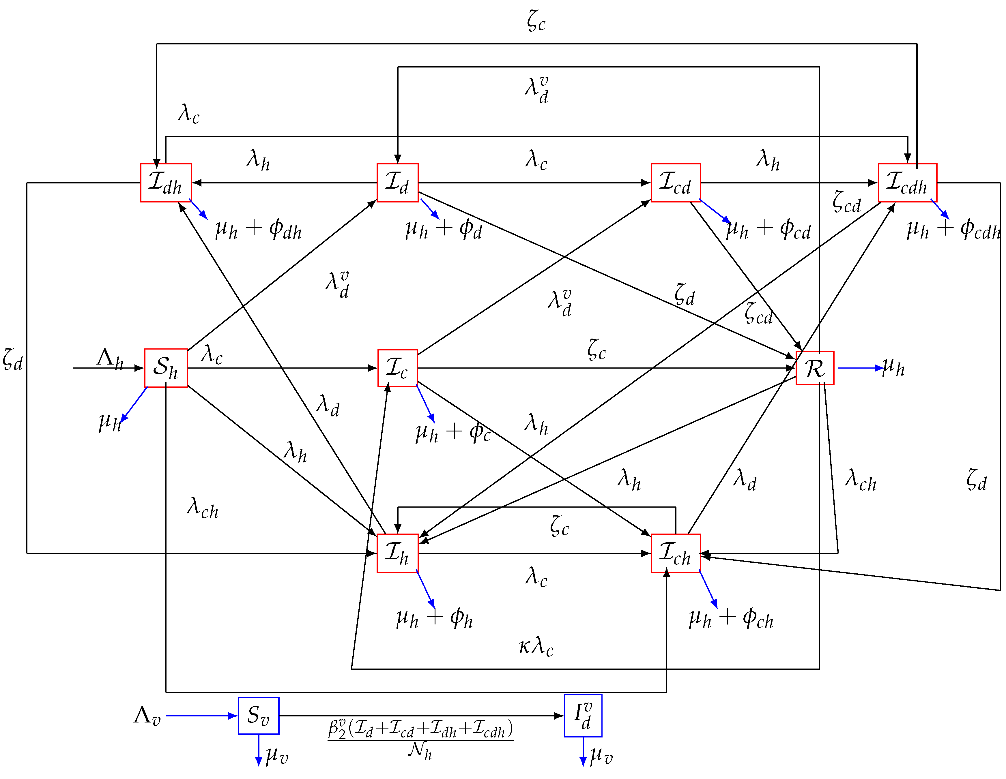
2. Model Formulation

The total population at any time t is denoted by N h ( t ) and comprises susceptible or vulnerable humans S h ( t ) ; COVID-19 infected I c ( t ) ; dengue infected I d ( t ) ; HIV infected I h ( t ) , COVID-19 and dengue infected I c d ( t ) ; COVID-19 and HIV infected I c h ( t ) ; dengue and HIV infected I d h ( t ) ; and COVID-19, dengue, and HIV infected I c d h ( t ) , with R ( t ) standing for COVID-19 or dengue recovered individuals. The total mosquito population N v ( t ) ( t ) comprises susceptible or uninfected mosquitoes: S v ( t ) and infected mosquitoes with dengue, I d v ( t ) . Recruitment into the human environment is represented by Λ h . Susceptible or uninfected persons S h can become infected with any of the three infections at the rates β 1 ( I c + I c d + I c h + I c d h ) N h , β 2 h I d v N h , β 3 ( I h + I c h + I d h + I c d h ) N h , respectively. We have also assumed concurrent transmission of COVID-19 and HIV at the rate β 13 I c h N h . The term μ h is the natural death rate. Individuals in the COVID-19-infected stage, dengue-infected, and HIV-infected compartments may die due to the diseases at the rates ϕ c , ϕ d , and ϕ h , respectively. Individuals in the COVID-19-infected class can also become co-infected with either dengue or HIV at the rates β 2 h I d v N h and β 3 ( I h + I c h + I d h + I c d h ) N h , respectively. Similarly, those infected with dengue or HIV can become infected with COVID-19 at the rate β 1 ( I c + I c d + I c h + I c d h ) N h . Individuals co-infected with COVID-19 and dengue can become infected with HIV at the rate β 3 ( I h + I c h + I d h + I c d h ) N h . Those infected with COVID-19 and HIV can become infected with dengue at the rate β 2 h I d v N h , while those infected with dengue and HIV can also become infected with COVID-19 at the rate β 1 ( I c + I c d + I c h + I c d h ) N h . Recovery rates for dengue- and COVID-19-infected individuals are defined by ζ d and ζ c , respectively. We have also assumed that after recovery from COVID-19, an individual has some immunity against re-infection [38], with κ denoting the COVID-19 re-infection rate. However, recovery from dengue does not confer any immunity, and an individual can become re-infected, just like the susceptibles. Recovered individuals are also susceptible to HIV infection. In addition, we have assumed co-infection with the three diseases, which is possible [39]. Moreover, concurrent transmission of either COVID-19 and dengue or HIV and dengue is not captured in the model, as it has not yet been clinically documented whether a mosquito or human can transmit COVID-19 and dengue or HIV and dengue concurrently.
In order to avoid complications in the model, asymptomatic classes for either COVID-19 or dengue were not assumed. The model also considered only the HIV infection stage, without assuming the full-blown AIDS stage. Although the authors recognize that asymptomatic individuals could play a crucial role in the transmission dynamics of infectious diseases, by omitting asymptomatic classes, the model fails to capture the full spectrum of disease severity and transmission patterns. This could also result in an incomplete representation of the interactions between the three viral diseases and their impact on the population. By excluding asymptomatic individuals and those with full-blown AIDS, the model may underestimate the true burden of each disease and their interactions. Individuals with full-blown AIDS may experience different clinical outcomes and interactions with COVID-19 and dengue compared to those with HIV infection alone. The authors also acknowledge that the findings of this study may have limited generalizability to real-world scenarios, since asymptomatic individuals and those with full-blown AIDS are excluded. Thus, future work in this regard is desirable, to fill the research gap that this study has created. Moreover, there is not much information available regarding vaccine or infection-acquired cross-protection between COVID-19, HIV, and dengue. There is no detailed clinical information on whether the currently available COVID-19 or dengue vaccines could cross-protect against infection with HIV. It should be stated that understanding the potential cross-protection between vaccines for COVID-19, dengue, and HIV is crucial. Future research will focus on evaluating the potential cross-reactivity or immune interactions between vaccines, exploring whether vaccination against one disease could provide a degree of cross-protection against the other two, and assessing the potential impacts on disease severity and transmission dynamics. The model parameters and flow chart (describing other transitions in the model) are presented in Table 1 and Figure 1, respectively.
d S h d t = Λ h β 1 ( I c + I c d + I c h + I c d h ) N h + β 2 h I d v N h + β 3 ( I h + I c h + I d h + I c d h ) N h + β 13 I c h N h + μ h S h , d I c d t = β 1 ( I c + I c d + I c h + I c d h ) N h ( S h + κ R ) ϕ c + ζ c + μ h I c β 2 h I d v N h I c β 3 ( I h + I c h + I d h + I c d h ) N h I c , d I d d t = β 2 h I d v N h ( S h + R ) ϕ d + ζ d + μ h I d β 1 ( I c + I c d + I c h + I c d h ) N h I d β 3 ( I h + I c h + I d h + I c d h ) N h I d , d I h d t = β 3 ( I h + I c h + I d h + I c d h ) N h ( S h + R ) + ζ c I c h + ζ d I d h + ζ c d I c d h ϕ h + μ h I h β 1 ( I c + I c d + I c h + I c d h ) N h I h β 2 h I d v N h I h , d I c d d t = β 2 h I d v N h I c + β 1 ( I c + I c d + I c h + I c d h ) N h I d ϕ c d + ζ c d + μ h I c d β 3 ( I h + I c h + I d h + I c d h ) N h I c d , d I c h d t = β 13 I c h N h ( S h + R ) + β 3 ( I h + I c h + I d h + I c d h ) N h I c + β 1 ( I c + I c d + I c h + I c d h ) N h I h + ζ d I c d h ϕ c h + ζ c + μ h I c h β 2 h I d v N h I c h , d I d h d t = β 3 ( I h + I c h + I d h + I c d h ) N h I d + β 2 h I d v N h I h + ζ c I c d h ϕ d h + ζ d + μ h I d h β 1 ( I c + I c d + I c h + I c d h ) N h I d h , d I c d h d t = β 3 ( I h + I c h + I d h + I c d h ) N h I c d + β 2 h I d v N h I c h + β 1 ( I c + I c d + I c h + I c d h ) N h I d h ϕ c d h + ζ c + ζ d + ζ c d + μ h I c d h , d R d t = ζ c I c + ζ d I d + ζ c d I c d κ β 1 ( I c + I c d + I c h + I c d h ) N h + β 2 h I d v N h + β 3 ( I h + I c h + I d h + I c d h ) N h + β 13 I c h N h + μ h R , d S v d t = Λ v β 2 v ( I d + I c d + I d h + I c d h ) N h + μ v S v , d I d v d t = β 2 v ( I d + I c d + I d h + I c d h ) N h S v μ v I d v .

3. Analysis of the Model

A qualitative analysis of the formulated model without controls is carried out in this section.

3.1. Non-Negativity of the Model Solutions

In order for system (1) to be epidemiologically meaningful, it is necessary to show that the solutions are non-negative over the passage of time. This result is established thus:
Theorem 1.
Given the initial states S h ( 0 ) 0 , I c ( 0 ) 0 , I d ( 0 ) 0 , I h ( 0 ) 0 , I c d ( 0 ) 0 , I c h ( 0 ) 0 , I d h ( 0 ) 0 , I c d h ( 0 ) 0 , R ( 0 ) 0 , S v ( 0 ) 0 , I d v ( 0 ) 0 .
Then the solutions, ( S h ( t ) , I c ( t ) , I d ( t ) , I h ( t ) , I c d ( t ) , I c h ( t ) , R ( t ) , S v ( t ) , I d v ( t ) ) of system (1) are non-negative for all time t > 0 .
Proof. 
The 1st Equation of (1) is given by
d S h ( t ) d t = Λ h ( λ c ( t ) + λ d v ( t ) + λ h ( t ) + λ c h ( t ) + μ h ) S h ,
where,
λ c ( t ) = β 1 ( I c + I c d + I c h + I c d h ) N h , λ d v ( t ) = β 2 h I d v N h , λ h = β 3 ( I h + I c h + I d h + I c d h ) N h , λ c h ( t ) = β 13 I c h N h .
Upon the application of the integrating factor approach in (2) we obtain
d d t S h ( t ) exp 0 t ( λ c ( σ ) + λ d v ( σ ) + λ h ( σ ) + λ c h ( σ ) ) d σ + μ h t = Λ h exp [ 0 t ( λ c ( σ ) + λ d v ( σ ) + λ h v ( σ ) + λ c h ( σ ) ) d σ + μ h t ] .
Integrating both sides of (3) gives
S h ( t ) exp 0 t ( λ c ( σ ) + λ d v ( σ ) + λ h ( σ ) + λ c h ( σ ) ) d σ + μ h t S ( 0 )
= Λ h 0 t exp 0 x ( λ c ( σ ) + λ d v ( σ ) + λ h ( σ ) + λ c h ( σ ) ) d σ + μ h x d x .
Thus,
S h ( t ) = S h ( 0 ) exp 0 t ( λ c ( σ ) + λ d v ( σ ) + λ h ( σ ) + λ c h ( σ ) ) d σ μ h t + exp 0 t ( λ c ( σ ) + λ d v ( σ ) + λ h ( σ ) + λ c h ( σ ) ) d σ μ h t × Λ h 0 t exp 0 x ( λ c ( σ ) + λ d v ( σ ) + λ h ( σ ) + λ c h ( σ ) ) d σ + μ h x d x 0 .
Hence, S h ( t ) 0 for a sufficiently large time t.
Similarly, it can be shown that
I c ( t ) 0 , I d ( t ) 0 , I h ( t ) 0 , I c d ( t ) 0 , I c h ( t ) 0 , I d h ( t ) 0 , I c d h ( t ) 0 , R ( t ) 0 , S v ( t ) 0 , I d v ( t ) 0 . □

3.2. Boundedness of the Solution

Theorem 2.
The closed set D = D × D v , with
D = ( S h , I c , I d , I h , I c d , I c h , I d h , I c d h , R ) R + 9 : S h + I c + I d + I h + I c d + I c h + I d h + I c d h + R Λ h μ h ,
D v = ( S v , I d v ) R + 2 : S v + I d v Λ v μ v .
is positively invariant relative to model (1).
Proof. 
If all the equations associated with human components are added up, this gives
d N h d t = Λ h μ h N h ( t ) [ ϕ c I c + ϕ d I d + ϕ h I h + ϕ c d I c d + ϕ c h I c h + ϕ d h I d h + ϕ c d h I c d h ] .
Equation (4) can be re-written as
d N h d t Λ h μ h N h ,
that is,
d N h ( t ) d t + μ h N h ( t ) Λ h ,
Upon application of the integrating factor approach in (6) and simplification, we obtain the inequality
N h ( t ) Λ h μ h + N h ( 0 ) Λ h μ h e μ h t ,
which further implies that
lim sup t N h ( t ) Λ h μ h .
Thus, N h ( t ) Λ h μ h for a sufficiently large t.
Similarly, N v ( t ) Λ v μ v . Therefore, it is concluded that the system (1) is positively invariant. □

3.3. The Basic Reproduction Number of the Model

The model’s DFE (disease-free equilibrium) is given by
M 0 = S h * , I c * , I d * , I h * , I c d * , I c h * , I d h * , I c d h * R * , S v * , I d v * = Λ h μ h , 0 , 0 , 0 , 0 , 0 , 0 , 0 , 0 , Λ v μ v , 0 .
The next generation operator approach [46] can be applied to system (1) to obtain the reproduction number. The transfer matrices, whose dimensions correspond to the number of infected classes of the model, that is: I c , I d , I h , I c d , I c h , I d h , I c d h , I d v are defined below:
F = β 1 0 0 β 1 β 1 0 β 1 0 0 0 0 0 0 0 0 β 2 h 0 0 β 3 0 β 3 β 3 β 3 0 0 0 0 0 0 0 0 0 0 0 0 0 β 13 0 0 0 0 0 0 0 0 0 0 0 0 0 0 0 0 0 0 0 0 β 2 v S v * N h * 0 β 2 v S v * N h * 0 β 2 v S v * N h * β 2 v S v * N h * 0 , V = H 1 0 0 0 0 0 0 0 0 H 2 0 0 0 0 0 0 0 0 H 3 0 ζ c ζ d ζ c d 0 0 0 0 H 4 0 0 0 0 0 0 0 0 H 5 0 ζ d 0 0 0 0 0 0 H 6 ζ c 0 0 0 0 0 0 0 H 7 0 0 0 0 0 0 0 0 μ v ,
where
H 1 = ϕ c + ζ c + μ h , H 2 = ϕ d + ζ d + μ h , H 3 = ϕ h + μ h , H 4 = ϕ c d + ζ c d + μ h , H 5 = ϕ c h + ζ c + μ h , H 6 = ϕ d h + ζ d + μ h , H 7 = ϕ c d h + ζ c + ζ d + ζ c d + μ h .
The reproduction number for system (1) is given by R 0 = ρ ( F V 1 ) = max { R 0 c , R 0 d , R 0 h , R 0 c h } where R 0 c , R 0 d , R 0 h and R 0 c h are the reproduction numbers for COVID-19, dengue, HIV, and co-infection (of COVID-19 and HIV), respectively, given by
R 0 c = β 1 ( ϕ c + ζ c + μ h ) , R 0 d = β 2 h β 2 v μ h Λ v Λ h μ v 2 ( ϕ d + ζ d + μ h ) , R 0 h = β 3 ( ϕ h + μ h ) , R 0 c h = β 13 ( ϕ c h + ζ c + μ h ) .

3.4. Local Asymptotic Stability of the Disease Free Equilibrium (DFE) of the Model

Theorem 3.
The model’s DFE, M 0 , is locally asymptotically stable given that R 0 < 1 , and unstable given that R 0 > 1 .
Proof. 
The Jacobian matrix of system (1) computed at the DFE M 0 is given by
μ h β 1 0 β 3 β 1 ( β 1 + β 3 + β 13 ) β 3 ( β 1 + β 3 ) 0 0 β 2 h 0 β 1 H 1 0 0 β 1 β 1 0 β 1 0 0 0 0 0 H 2 0 0 0 0 0 0 0 β 2 h 0 0 0 β 3 H 3 0 β 3 β 3 β 3 + ζ c 0 0 0 0 0 0 0 H 4 0 0 0 0 0 0 0 0 0 0 0 β 13 H 5 0 ζ d 0 0 0 0 0 0 0 0 0 H 6 ζ c 0 0 0 0 0 0 0 0 0 0 H 7 0 0 0 0 ζ c ζ d 0 ζ c d 0 0 0 μ h 0 0 0 0 β 2 v S v * N h * 0 β 2 v S v * N h * 0 β 2 v S v * N h * β 2 v S v * N h * 0 μ v 0 0 0 β 2 v S v * N h * 0 β 2 v S v * N h * 0 β 2 v S v * N h * β 2 v S v * N h * 0 0 μ v .
The eigenvalues are given by
ϱ 1 = ( ϕ c d + ζ c d + μ h ) , ϱ 2 = ( ϕ d h + ζ d + μ h ) , ϱ 3 = ( ϕ c d h + ζ c + ζ d + ζ c d + μ h ) , ϱ 4 = μ h ( with multiplicity of 2 ) , ϱ 5 = μ v ,
and the zeros of the equations
ϱ + H 1 ( 1 R 0 c ) = 0 ,
ϱ + H 3 ( 1 R 0 h ) = 0 ,
ϱ + H 5 ( 1 R 0 c h ) = 0 ,
ϱ 2 + ( μ v + H 2 ) ϱ + μ v H 2 ( 1 R 0 d 2 ) = 0 .
Adopting the Routh–Hurwitz criterion, all four Equations (12)–(15) possess zeros having negative real parts if, and only if, the reproduction numbers R 0 c < 1 , R 0 d < 1 , R 0 h < 1 and R 0 c h < 1 . Hence, the DFE M 0 is locally asymptotically stable if R 0 = max { R 0 c , R 0 d , R 0 h , R 0 c h } < 1 . □

3.5. Backward Bifurcation Analysis of the Model

In this section, we will carry out a backward bifurcation analysis of the model. The center-manifold theory [47] (given in Appendix A) will be employed for this purpose.
We found the results below:
Theorem 4.
The co-dynamical model (1) will exhibit backward bifurcation if
a = 2 ( ω 2 + ω 3 + ω 4 ) ( β 1 ω 2 ν 2 β 2 h ω 11 ν 3 ) + 2 ω 9 ( κ β 1 ω 2 ν 2 + β 2 ω 11 ν 3 ) N h * 2 β 1 ( ω 2 + ω 6 ) [ ω 3 ν 3 + ω 4 ν 4 ω 3 ν 5 ω 4 ν 6 + ω 7 ν 7 ω 7 ν 8 ] N h * β 3 ( ω 4 + ω 6 ) [ ω 4 ν 3 + ( ω 2 + ω 3 + ω 4 + ω 6 + ω 9 ) ν 4 ω 9 ν 4 + ω 5 ν 5 ω 2 ν 6 ω 3 ν 7 ω 5 ν 8 ] N h * 2 β 13 ( ω 3 + ω 6 ) ω 6 ν 6 N h * 2 β 2 v x 10 * ( ω 3 + ω 8 ) ( ω 1 + ω 2 + ω 3 + ω 4 + ω 6 + ω 9 ) ν 11 N h * 2 2 β 2 h ω 11 ( ω 4 ν 4 + ω 2 ν 5 + ω 6 ν 6 ω 4 ν 7 ) N h * + 2 β 2 v ω 3 ω 10 ν 11 N h * > 0 ,
where ω 1 , ω 2 , ω 3 , , ω 11 and ν 1 , ν 2 , ν 3 , , ν 11 represent the right and left eigenvector components, associated with the simple zero eigenvalues of the Jacobian matrix (11) evaluated at the infection-free equilibrium, M 0 given in (8). The other parameters are the same as defined in Table 1.
Proof. 
Consider the case when R 0 = max { R 0 c , R 0 d , R 0 h , R 0 c h } = 1 . Suppose, further, that a contact rate, say β 13 , is chosen as a bifurcation parameter. Solving for β 13 = β 13 * from R 0 c h = 1 gives
β 13 = β 13 * = H 5 .
Using the approach in [47], the Jacobian matrix J ( M 0 ) given in (11) has a right eigenvector (linked with the zero eigenvalues of J ( M 0 ) ) given by ω = ω 1 , ω 2 , ω 3 , , ω 11 T , where the components are
ω 1 = 1 μ h β 1 ( ω 2 + ω 5 + ω 6 ) + β 3 ( ω 4 + ω 6 ) + β 13 ω 6 + β 2 h ω 11 < 0 , ω 2 = β 1 H 1 > 0 , ω 3 = β 2 h ω 11 H 2 > 0 , ω 4 = ω 4 > 0 , ω 5 = 0 , ω 6 = ω 6 > 0 , ω 7 = ω 8 = 0 , ω 9 = 1 μ ( ζ c ω 2 + ζ d ω 3 ) > 0 , ω 10 = 1 μ v β 2 v ω 3 N h * = < 0 , ω 11 = 1 μ v β 2 v ω 3 N h * > 0 .
The non-zero components of the left eigenvector of J ( M 0 ) | β 13 = β 13 * , ν = [ ν 1 , ν 2 , , ν 11 ] , satisfying ω . ν = 1 are
ν 1 = 0 , ν 2 = ν 2 > 0 , ν 3 = β 2 v S v * μ v H 2 N h * > 0 , ν 4 = ν 4 > 0 , ν 5 = 1 H 4 β 1 ν 2 + H 2 β 2 h > 0 , ν 6 = ν 6 > 0 , ν 7 = 1 H 6 β 3 ν 4 + H 2 β 2 h > 0 , ν 8 = 1 H 7 β 1 ν 2 + ( β 3 + ζ c ) ν 4 + ζ d ν 6 + ζ c ν 7 + H 2 β 2 h > 0 , ν 9 = ν 10 = 0 , ν 11 = H 2 N h * β 2 h β 2 v S v * > 0 .
Applying Theorem 4.1 in [47] and by computing the non-trivial partial differentiations of f ( x ) (evaluated at DFE, ( M 0 )), the coefficients defined as
a = k , i , j = 1 11 ν k ω i ω j 2 f k x i x j ( 0 , 0 ) and b = k , i = 1 11 ν k ω i 2 f k x i β 3 h * ( 0 , 0 ) ,
are computed to be
a = 2 ( ω 2 + ω 3 + ω 4 ) ( β 1 ω 2 ν 2 β 2 h ω 11 ν 3 ) + 2 ω 9 ( κ β 1 ω 2 ν 2 + β 2 ω 11 ν 3 ) N h * 2 β 1 ( ω 2 + ω 6 ) [ ω 3 ν 3 + ω 4 ν 4 ω 3 ν 5 ω 4 ν 6 + ω 7 ν 7 ω 7 ν 8 ] N h * β 3 ( ω 4 + ω 6 ) [ ω 4 ν 3 + ( ω 2 + ω 3 + ω 4 + ω 6 + ω 9 ) ν 4 ω 9 ν 4 + ω 5 ν 5 ω 2 ν 6 ω 3 ν 7 ω 5 ν 8 ] N h * 2 β 13 ( ω 3 + ω 6 ) ω 6 ν 6 N h * 2 β 2 v S v * ( ω 3 + ω 8 ) ( ω 1 + ω 2 + ω 3 + ω 4 + ω 6 + ω 9 ) ν 11 N h * 2 2 β 2 h ω 11 ( ω 4 ν 4 + ω 2 ν 5 + ω 6 ν 6 ω 4 ν 7 ) N h * + 2 β 2 v ω 3 ω 10 ν 11 N h * , b = ω 6 ν 6 > 0 .
It can be observed that the backward bifurcation coefficient b is strictly greater than zero. Thus, it is concluded, following [47], that the model (1) would undergo backward bifurcation when the coefficient a > 0 . The epidemiological significance of the backward bifurcation phenomenon of system (1) is that the classical necessity of having the reproduction number R 0 less than unity, even though still necessary, is no longer sufficient for effective elimination of the diseases. □

3.6. Global Asymptotic Stability (GAS) of the Disease-Free Equilibrium for a Special Case

Studying the global properties of a full co-infection model can be difficult, due to the strong non-linearity of the model. We shall thus consider a special case of the model when there is no co-infection or re-infection with the same or a different disease. The reduced model under this scenario is given below:
d S h d t = Λ h β 1 I c N h + β 2 h I d v N h + β 3 I h N h + μ h S h , d I c d t = β 1 I c N h S h ϕ c + ζ c + μ h I c , d I d d t = β 2 h I d v N h S h ϕ d + ζ d + μ h I d , d I h d t = β 3 I h N h S h ϕ h + μ h I h , d R d t = ζ c I c + ζ d I d μ h R , d S v d t = Λ v β 2 v I d N h S v μ v S v , d I d v d t = β 2 v I d N h S v μ v I d v .
Furthermore, consider the Lyapunov function candidate defined below:
Z 1 = ln ( S h S h * ) + I c + I d + I h + R + ( S v S v * ) + I d v + 1 H 1 I c + β 2 v S v * μ v H 2 I d + 1 H 3 I h + R 0 d μ v I d v ,
where S h * , S v * , H 1 , H 2 , and H 3 are given by Equations (8) and (10).
The Lyapunov time derivative of (17)
Z ˙ 1 = 1 ( S h S h * ) + I c + I d + I h + R + ( S v S v * ) + I d v ( Λ h β 1 I c N h + β 2 h I d v N h + β 3 I h N h + μ h S h + β 1 I c N h S h ϕ c + ζ c + μ h I c + β 2 h I d v N h S h ϕ d + ζ d + μ h I d + β 3 I h h N h S h ϕ h + μ h I h + ζ c I c + ζ d I d μ h R + Λ v β 2 v I d N h + μ v S v + β 2 v I d N h S v μ v I d v ) + 1 H 1 β 1 I c N h S h ϕ c + ζ c + μ h I c + β 2 v S v * μ v H 2 β 2 h I d v N h S h ϕ d + ζ d + μ h I d + 1 H 3 β 3 I h N h S h ϕ h + μ h I h + R 0 d μ v β 2 v I d N h S v μ v I d v ,
which can be further simplified into
Z ˙ 1 = 1 ( S h S h * ) + I c + I d + I h + R + ( S v S v * ) + I d v ( Λ h μ h ( S h + I c + I d + I h + R ) + Λ v μ v ( S v + I d v ) ( ϕ c I c + ϕ d I d + ϕ h I h ) ) + 1 H 1 β 1 I c N h S h H 1 I c + β 2 v S v * μ v H 2 β 2 h I d v N h S h H 2 I d + 1 H 3 β 3 I h N h S h H 3 I h + R 0 d μ v β 2 v I d N h S v μ v I d v .
Simplifying further (noting that S h + I c + I d + I h + R Λ h μ h , S v + I d v Λ v μ v , and S v < S v * ), we have
Z ˙ 1 ( ϕ c I c + ϕ d I d + ϕ h I h ) ( S h S h * ) + I c + I d + I h + R + ( S v S v * ) + I d v + 1 H 1 β 1 I c S h * N h * H 1 I c + β 2 v S v * μ v H 2 β 2 h I d v S h * N h * H 2 I d + 1 H 3 β 3 I h S h * N h * H 3 I h + R 0 d μ v β 2 v I d S v * N h * μ v I d v , = ( ϕ c I c + ϕ d I d + ϕ h I h ) ( S h S h * ) + I c + I d + I h + R + ( S v S v * ) + I d v + β 1 ( ϕ c + ζ c + μ h ) 1 I c + β 2 v S v * μ v β 2 h β 2 v μ h Λ v Λ h μ v 2 ( ϕ d + ζ d + μ h ) 1 I d + β 2 h β 2 v μ h Λ v Λ h μ v 2 ( ϕ d + ζ d + μ h ) R 0 d I d v + β 3 ( ϕ h + μ h ) 1 I h = ( ϕ c I c + ϕ d I d + ϕ h I h ) ( S h S h * ) + I c + I d + I h + R + ( S v S v * ) + I d v + ( R 0 c 1 ) I c + β 2 v S v * μ v ( R 0 d 1 ) I d + R 0 d ( R 0 d 1 ) I d v + ( R 0 h 1 ) I h .
Noting that all the parameters and variables are not less than zero, it can be concluded that Z ˙ 1 < 0 for R 0 = max { R 0 c , R 0 d , R 0 h , R 0 c h } 1 . Thus, L is an appropriate Lyapunov candidate on Q (the DFE of model (16)). As a result, the DFE is globally asymptotically stable [48].

3.7. Global Asymptotic Stability (GAS) of the Endemic Equilibrium Point (EEP) of the Model (1)

Theorem 5.
Suppose that we assume infection-acquired immunity against re-infection with the same or a different disease and the absence of co-infection and super-infection in the model (1). Then, the model’s endemic equilibrium, given by Q e , is GAS in D , given that R 0 > 1 .
Proof. 
Consider the non-linear Lyapunov function:
Z 2 = β 2 v S v * * μ v H 2 S h S h * * S h * * ln S h S h * * + I c I c * * I c * * ln I c I c * * + I d I d * * I d * * ln I d I d * * + I h I h * * I h * * ln I h I h * * + H 2 β 2 h β 2 v S h * * S v * * S v S v * * S v * * ln S v S v * * + I d v I d v * * I d v * * ln I d v I d v * * ,
where the terms in * * denote the solutions of system (16) at the endemic equilibrium:
Λ h = β 1 I c * * N h * * + β 2 h I d v * * N h * * + β 3 I h * * N h * * + μ h S h * * β 1 I c * * N h * * S h * * = ϕ c + ζ c + μ h I c * * β 2 h I d v * * N h * * S h * * = ϕ d + ζ d + μ h I d * * β 3 I h * * N h * * S h * * = ϕ h + μ h I h * * ζ c I c * * + ζ d I d * * = μ h R * * Λ v = β 2 v I d * * N h * * + μ v S v * * β 2 v I d * * N h * * S v * * = μ v I d v * *
The Lyapunov time derivative of (18) is given by:
Z ˙ 2 = β 2 v S v * * μ v H 2 1 S h * * S h S h ˙ + 1 I c * * I c I ˙ c + 1 I d * * I d I ˙ d + H 2 β 2 h β 2 v S h * * S v * * 1 S v * * S v S v ˙ + 1 I d v * * I d v I ˙ d v
Substituting the derivatives in (16) into Z ˙ 2 , we have
Z ˙ 2 = β 2 v S v * * μ v H 2 1 S h * * S h Λ h β 1 I c N h + β 2 h I d v N h + β 3 I h N h + μ h S h + β 2 v S v * * μ v H 2 1 I c * * I c β 1 I c N h S h ϕ c + ζ c + μ h I c + β 2 v S v * * μ v H 2 1 I d * * I d β 2 h I d v N h S h ϕ d + ζ d + μ h I d + β 2 v S v * * μ v H 2 1 I h * * I h β 3 I h N h S h ϕ h + μ h I h + H 2 β 2 h β 2 v S h * * S v * * 1 S v * * S v Λ v β 2 v I d N h + μ v S v + H 2 β 2 h β 2 v S h * * S v * * 1 I d v * * I d v β 2 v I d N h S v μ v I d v .
Substituting the expressions in (19) into (21) gives
Z ˙ 2 = β 2 v S v * * μ v H 2 1 S h * * S h β 1 I c * * N h * * + β 2 h I d v * * N h * * + β 3 I h * * N h * * + μ h S h * * β 1 I c N h * * + β 2 h I d v N h * * + β 3 I h N h * * + μ h S h + β 2 v S v * * μ v H 2 1 I c * * I c β 1 I c N h * * S h ϕ c + ζ c + μ h I c + β 2 v S v * * μ v H 2 1 I d * * I d β 2 h I d v N h * * S h ϕ d + ζ d + μ h I d + β 2 v S v * * μ v H 2 1 I h * * I h β 3 I h N h * * S h ϕ h + μ h I h + H 2 β 2 h β 2 v S h * * S v * * 1 S v * * S v β 2 v I d * * N h * * + μ v S v * * β 2 v I d N h * * + μ v S v + H 2 β 2 h β 2 v S h * * S v * * 1 I d v * * I d v β 2 v I d N h * * S v μ v I d v ,
which can be re-written as
Z ˙ 2 = β 2 v S v * * μ v H 2 1 S h * * S h β 1 I c * * + β 2 h I d v * * + β 3 I h * * + μ h S h * * β 1 I c + β 2 h I d v + β 3 I h + μ h S h + β 2 v S v * * μ v H 2 1 I c * * I c β 1 I c S h ϕ c + ζ c + μ h I c + β 2 v S v * * μ v H 2 1 I d * * I d β 2 h I d v S h ϕ d + ζ d + μ h I d + β 2 v S v * * μ v H 2 1 I h * * I h β 3 I h S h ϕ h + μ h I h + H 2 β 2 h β 2 v S h * * S v * * 1 S v * * S v β 2 v I d * * + μ v S v * * β 2 v I d + μ v S v + H 2 β 2 h β 2 v S h * * S v * * 1 I d v * * I d v β 2 v I d S v μ v I d v ,
which after some algebraic manipulations is simplified to
Z ˙ 2 = β 2 v S v * * μ v H 2 [ 2 μ h S h * * μ h S h μ h S h * * 2 S h + 2 β 1 I c * * S h * * + 2 β 2 h I d v * * S h * * + 2 β 3 I h * * S h * * β 1 I c * * S h * * 2 S h β 1 I c * * S h β 2 h I d v * * S h * * 2 S h β 2 h I d v I d * * S h I d β 3 I h * * S h * * 2 S h β 3 I h * * S h ] + H 2 β 2 h β 2 v S h * * S v * * 2 μ v S v * * μ v S v μ v S v * * 2 S v + 2 β 2 v I d * * S v * * β 2 v I d * * S v * * 2 S v β 2 v I d I d v * * S v I d v .
The above can be simplified to
Z ˙ 2 = μ h β 2 v S h * * S v * * μ v H 2 S h * * 2 S h * * S h S h S h * * + μ v H 2 β 2 h β 2 v S h * * 2 S v * * S v S v S v * * β 1 β 2 v S h * * S v * * I c * * μ v H 2 2 S h * * S h S h S h * * + β 2 v β 3 S h * * S v * * I h * * μ v H 2 2 S h * * S h S h S h * * + β 2 h β 2 v S h * * S v * * I d v * * μ v H 2 4 S h * * S h S v * * S v S h I d v I d * * S h * * I d v * * I d S v I d v * * I d S v * * I d v I d * * .
As the arithmetic mean is greater than the geometric mean, the following inequalities from (23) hold:
2 S h * * S h S h S h * * 0 , 2 S v * * S v S v S v * * 0 , 4 S h * * S h S v * * S v S h I d v I d * * S h * * I d v * * I d S v I d v * * I d S v * * I d v I d * * 0 .
Hence, Z 2 ˙ 0 for R 0 > 1 . Therefore, Z 2 is a Lyapunov candidate in D D 0 and it is concluded that the GAS of EEP is globally asymptotically stable for R 0 > 1 . □

4. Optimal Control Analysis

In this section, time dependent controls will be considered for the model (1), in order to obtain the optimal strategies for the control of the three diseases. They are defined as follows:
  • u 1 : COVID-19 prevention control: this represents all the efforts towards COVID-19 prevention (and these include COVID-19 vaccination, face-mask usage in public, use of personal protective equipment (PPE) by health personnel, etc.);
  • u 2 : Dengue prevention control: this represents all the efforts to prevent mosquito transmission of dengue disease. These include minimizing, as much as possible, the contacts between mosquitoes and humans, use of treated bed nets, and also receiving dengue vaccination;
  • u 3 : HIV prevention control: This involves efforts to prevent HIV transmission via abstinence and effective condom use by sexually active individuals;
  • u 4 : Control against co-infection: this involves combined efforts against all co-infections (COVID-19/dengue, COVID-19/HIV, dengue/HIV as well as COVID-19/dengue/HIV).
The optimal control problem assesses the scenarios where the number of infections, as well as the cost of implementing the above preventive controls, u 1 , u 2 , u 3 , and u 4 , are minimized subject to system (24). We have assumed that the above defined controls may or may not be 100% effective in preventing infections. Therefore, they are bounded thus: 0 < u 1 , u 2 , u 3 , u 4 1.0 . However, it is recommended that policies should be put in place to step up preventive efforts at a very high level, so as to sufficiently reduce the co-spread of the diseases under investigation.
The optimal system is thus given by
d S h d t = Λ h ( ( 1 u 1 ) β 1 ( I c + I c d + I c h + I c d h ) N h + ( 1 u 2 ) β 2 h I d v N h + ( 1 u 3 ) β 3 ( I h + I c h + I d h + I c d h ) N h + ( 1 u 4 ) β 13 I c h N h + μ h ) S h , d I c d t = ( 1 u 1 ) β 1 ( I c + I c d + I c h + I c d h ) N h ( S h + κ R ) ϕ c + ζ c + μ h I c ( 1 u 4 ) β 2 h I d v N h I c ( 1 u 4 ) β 3 ( I h + I c h + I d h + I c d h ) N h I c , d I d d t = ( 1 u 2 ) β 2 h I d v N h ( S h + R ) ϕ d + ζ d + μ h I d ( 1 u 4 ) β 1 ( I c + I c d + I c h + I c d h ) N h I d ( 1 u 4 ) β 3 ( I h + I c h + I d h + I c d h ) N h I d , d I h d t = ( 1 u 3 ) β 3 ( I h + I c h + I d h + I c d h ) N h ( S h + R ) + ζ c I c h + ζ d I d h + ζ c d I c d h ϕ h + μ h I h ( 1 u 4 ) β 1 ( I c + I c d + I c h + I c d h ) N h I h ( 1 u 4 ) β 2 h I d v N h I h , d I c d d t = ( 1 u 4 ) β 2 h I d v N h I c + ( 1 u 4 ) β 1 ( I c + I c d + I c h + I c d h ) N h I d ϕ c d + ζ c d + μ h I c d ( 1 u 4 ) β 3 ( I h + I c h + I d h + I c d h ) N h I c d , d I c h d t = ( 1 u 4 ) β 13 I c h N h ( S h + R ) + ( 1 u 4 ) β 3 ( I h + I c h + I d h + I c d h ) N h I c + ( 1 u 4 ) β 1 ( I c + I c d + I c h + I c d h ) N h I h + ζ d I c d h ϕ c h + ζ c + μ h I c h ( 1 u 4 ) β 2 h I d v N h I c h , d I d h d t = ( 1 u 4 ) β 3 ( I h + I c h + I d h + I c d h ) N h I d + ( 1 u 4 ) β 2 h I d v N h I h + ζ c I c d h ϕ d h + ζ d + μ h I d h ( 1 u 4 ) β 1 ( I c + I c d + I c h + I c d h ) N h I d h , d I c d h d t = ( 1 u 4 ) β 3 ( I h + I c h + I d h + I c d h ) N h I c d + ( 1 u 4 ) β 2 h I d v N h I c h + ( 1 u 4 ) β 1 ( I c + I c d + I c h + I c d h ) N h I d h ϕ c d h + ζ c + ζ d + ζ c d + μ h I c d h , d R d t = ζ c I c + ζ d I d + ζ c d I c d ( κ ( 1 u 1 ) β 1 ( I c + I c d + I c h + I c d h ) N h + ( 1 u 2 ) β 2 h I d v N h + ( 1 u 3 ) β 3 ( I h + I c h + I d h + I c d h ) N h + ( 1 u 4 ) β 13 I c h N h + μ h ) R , d S v d t = Λ v ( 1 u 2 ) β 2 v ( I d + I c d + I d h + I c d h ) N h + μ v S v , d I d v d t = ( 1 u 2 ) β 2 v ( I d + I c d + I d h + I c d h ) N h S v μ v I d v .
subject to the initial conditions
S h 0 = S h ( 0 ) , I c 0 = I c ( 0 ) , I d 0 = I d ( 0 ) , I h 0 = I h ( 0 ) , I c d 0 = I c d ( 0 ) , I c h 0 = I c h ( 0 ) , I d h 0 = I d h ( 0 ) , I c d h 0 = I c d h ( 0 ) , R 0 = R ( 0 ) , S v 0 = S v ( 0 ) , I d 0 v = I d v ( 0 ) .
We will consider the objective functional as follows:
J u 1 , u 2 , u 3 , u 4 = 0 T I c + I d + I h + I c d + I c h + I d h + I c d h + S v + I d v + ω 1 2 u 1 2 + ω 2 2 u 2 2 + ω 3 2 u 3 2 + ω 4 2 u 4 2 d t ,
where T is the final time. The total cost consists of the cost for COVID-19, dengue, and HIV preventive efforts, such as COVID-19 vaccination, treated bed nets for dengue, and condoms for HIV prevention. Thus, the nonlinear cost function has been assumed. We seek to find an optimal control quadruple, ( u 1 * , u 2 * , u 3 * , u 4 * ) , such that
J ( u 1 * , u 2 * , u 3 * , u 4 * ) = m i n { J ( u 1 , u 2 , u 3 , u 4 ) | u 1 , u 2 , u 3 , u 4 U } ,
where the control set U = { ( u 1 , u 2 , u 3 , u 4 ) : 0 u 1 ( t ) 1 , 0 u 2 ( t ) 1 , 0 u 3 ( t ) 1 , 0 u 4 ( t ) 1 for t [ 0 , T ] } , with u 1 , u 2 , u 3 , u 4 being Lebesgue measurable.
The Hamiltonian is defined by
X = I c + I d + I h + I c d + I c h + I d h + I c d h + S v + I d v + ξ 1 2 u 1 2 + ξ 2 2 u 2 2 + ξ 3 2 u 3 2 + ξ 4 2 u 4 2 + ϱ 1 ( Λ h ( ( 1 u 1 ) β 1 ( I c + I c d + I c h + I c d h ) N h + ( 1 u 2 ) β 2 h I d v N h + ( 1 u 3 ) β 3 ( I h + I c h + I d h + I c d h ) N h + ( 1 u 4 ) β 13 I c h N h + μ h ) S h ) + ϱ 2 ( ( 1 u 1 ) β 1 ( I c + I c d + I c h + I c d h ) N h ( S h + κ R ) ϕ c + ζ c + μ h I c ( 1 u 4 ) β 2 h I d v N h I c ( 1 u 4 ) β 3 ( I h + I c h + I d h + I c d h ) N h I c ) + ϱ 3 ( ( 1 u 2 ) β 2 h I d v N h ( S h + R ) ϕ d + ζ d + μ h I d ( 1 u 4 ) β 1 ( I c + I c d + I c h + I c d h ) N h I d ( 1 u 4 ) β 3 ( I h + I c h + I d h + I c d h ) N h I d ) + ϱ 4 ( ( 1 u 3 ) β 3 ( I h + I c h + I d h + I c d h ) N h ( S h + R ) + ζ c I c h + ζ d I d h + ζ c d I c d h ϕ h + μ h I h ( 1 u 4 ) β 1 ( I c + I c d + I c h + I c d h ) N h I h ( 1 u 4 ) β 2 h I d v N h I h ) + ϱ 5 ( ( 1 u 4 ) β 2 h I d v N h I c + ( 1 u 4 ) β 1 ( I c + I c d + I c h + I c d h ) N h I d ϕ c d + ζ c d + μ h I c d ( 1 u 4 ) β 3 ( I h + I c h + I d h + I c d h ) N h I c d ) + ϱ 6 ( ( 1 u 4 ) β 13 I c h N h ( S h + R ) + ( 1 u 4 ) β 3 ( I h + I c h + I d h + I c d h ) N h I c + ( 1 u 4 ) β 1 ( I c + I c d + I c h + I c d h ) N h I h + ζ d I c d h ϕ c h + ζ c + μ h I c h ( 1 u 4 ) β 2 h I d v N h I c h ) + ϱ 7 ( ( 1 u 4 ) β 3 ( I h + I c h + I d h + I c d h ) N h I d + ( 1 u 4 ) β 2 h I d v N h I h + ζ c I c d h ϕ d h + ζ d + μ h I d h ( 1 u 4 ) β 1 ( I c + I c d + I c h + I c d h ) N h I d h ) + ϱ 8 ( ( 1 u 4 ) β 3 ( I h + I c h + I d h + I c d h ) N h I c d + ( 1 u 4 ) β 2 h I d v N h I c h + ( 1 u 4 ) β 1 ( I c + I c d + I c h + I c d h ) N h I d h ϕ c d h + ζ c + ζ d + ζ c d + μ h I c d h ) + ϱ 9 ( ζ c I c + ζ d I d + ζ c d I c d ( κ ( 1 u 1 ) β 1 ( I c + I c d + I c h + I c d h ) N h + ( 1 u 2 ) β 2 h I d v N h + ( 1 u 3 ) β 3 ( I h + I c h + I d h + I c d h ) N h + ( 1 u 4 ) β 13 I c h N h + μ h ) R ) , + ϱ 10 Λ v ( 1 u 2 ) β 2 v ( I d + I c d + I d h + I c d h ) N h + μ v S v , + ϱ 11 ( 1 u 2 ) β 2 v ( I d + I c d + I d h + I c d h ) N h S v μ v I d v ,
where, ϱ 1 , ϱ 2 , , ϱ 11 represent the adjoint variables.

Existence

We report the results below:
Theorem 6.
Let J be defined on the control set U, subject to system (24) with non-negative initial conditions at t = 0 , then there exists an optimal control quadruple u * = ( u 1 * , u 2 * , u 3 * , u 4 * ) such that J ( u * ) = m i n J ( u 1 , u 2 , u 3 , u 4 ) | u 1 , u 2 , u 3 , u 4 U , if the following conditions proposed by [49] hold:
(i) 
The admissible control set U is convex and closed.
(ii) 
The state system is bounded by a linear function in the state and control variables.
(iii) 
The integrand of the objective functional in (26) is convex with respect to the controls.
(iv) 
The Lagrangian is no less than ϖ 1 | u | ϖ 3 ϖ 2 , where ϖ 1 > 0 , ϖ 2 > 0 , ϖ 3 > 1 .
Proof. 
Let U = [ 0 , 1 ] 4 be the control set, u = ( u 1 , u 2 , u 3 , u 4 ) U , x = ( S h , I c , I d , I h , I c d , I c h , I d h , I c d h , R , S v , I d v ) and f ( x , u ) be the right hand of (24), that is
f ( x , u ) = Λ h ( ( 1 u 1 ) β 1 ( I c + I c d + I c h + I c d h ) N h + ( 1 u 2 ) β 2 h I d v N h + ( 1 u 3 ) β 3 ( I h + I c h + I d h + I c d h ) N h + ( 1 u 4 ) β 13 I c h N h + μ h ) S h , ( 1 u 1 ) β 1 ( I c + I c d + I c h + I c d h ) N h ( S h + κ R ) ϕ c + ζ c + μ h I c ( 1 u 4 ) β 2 h I d v N h I c ( 1 u 4 ) β 3 ( I h + I c h + I d h + I c d h ) N h I c , ( 1 u 2 ) β 2 h I d v N h ( S h + R ) ϕ d + ζ d + μ h I d ( 1 u 4 ) β 1 ( I c + I c d + I c h + I c d h ) N h I d ( 1 u 4 ) β 3 ( I h + I c h + I d h + I c d h ) N h I d , ( 1 u 3 ) β 3 ( I h + I c h + I d h + I c d h ) N h ( S h + R ) + ζ c I c h + ζ d I d h + ζ c d I c d h ϕ h + μ h I h ( 1 u 4 ) β 1 ( I c + I c d + I c h + I c d h ) N h I h ( 1 u 4 ) β 2 h I d v N h I h , ( 1 u 4 ) β 2 h I d v N h I c + ( 1 u 4 ) β 1 ( I c + I c d + I c h + I c d h ) N h I d ϕ c d + ζ c d + μ h I c d ( 1 u 4 ) β 3 ( I h + I c h + I d h + I c d h ) N h I c d , ( 1 u 4 ) β 13 I c h N h ( S h + R ) + ( 1 u 4 ) β 3 ( I h + I c h + I d h + I c d h ) N h I c + ( 1 u 4 ) β 1 ( I c + I c d + I c h + I c d h ) N h I h + ζ d I c d h ϕ c h + ζ c + μ h I c h ( 1 u 4 ) β 2 h I d v N h I c h , ( 1 u 4 ) β 3 ( I h + I c h + I d h + I c d h ) N h I d + ( 1 u 4 ) β 2 h I d v N h I h + ζ c I c d h ϕ d h + ζ d + μ h I d h ( 1 u 4 ) β 1 ( I c + I c d + I c h + I c d h ) N h I d h , ( 1 u 4 ) β 3 ( I h + I c h + I d h + I c d h ) N h I c d + ( 1 u 4 ) β 2 h I d v N h I c h + ( 1 u 4 ) β 1 ( I c + I c d + I c h + I c d h ) N h I d h ϕ c d h + ζ c + ζ d + ζ c d + μ h I c d h , ζ c I c + ζ d I d + ζ c d I c d ( κ ( 1 u 1 ) β 1 ( I c + I c d + I c h + I c d h ) N h + ( 1 u 2 ) β 2 h I d v N h + ( 1 u 3 ) β 3 ( I h + I c h + I d h + I c d h ) N h + ( 1 u 4 ) β 13 I c h N h + μ h ) R , Λ v ( 1 u 2 ) β 2 v ( I d + I c d + I d h + I c d h ) N h + μ v S v , ( 1 u 2 ) β 2 v ( I d + I c d + I d h + I c d h ) N h S v μ v I d v .
To prove Theorem 6, we proceed as follows:
(i).
The convexity of set U is obvious since it is 4D parallelepiped [50].
(ii).
The control system (24) can be expressed as a linear function of control variables ( u 1 , u 2 , u 3 , u 4 ) , with the coefficients as functions of time and state variables:
f ( x , u ) = θ ( x ) + ϕ ( x ) u
with
θ ( x ) = Λ h β 1 ( I c + I c d + I c h + I c d h ) N h + β 2 h I d v N h + β 3 ( I h + I c h + I d h + I c d h ) N h + β 13 I c h N h + μ h S h , β 1 ( I c + I c d + I c h + I c d h ) N h ( S h + κ R ) ϕ c + ζ c + μ h I c β 2 h I d v N h I c β 3 ( I h + I c h + I d h + I c d h ) N h I c , β 2 h I d v N h ( S h + R ) ϕ d + ζ d + μ h I d β 1 ( I c + I c d + I c h + I c d h ) N h I d β 3 ( I h + I c h + I d h + I c d h ) N h I d , β 3 ( I h + I c h + I d h + I c d h ) N h ( S h + R ) + ζ c I c h + ζ d I d h + ζ c d I c d h ϕ h + μ h I h β 1 ( I c + I c d + I c h + I c d h ) N h I h β 2 h I d v N h I h , β 2 h I d v N h I c + β 1 ( I c + I c d + I c h + I c d h ) N h I d ϕ c d + ζ c d + μ h I c d β 3 ( I h + I c h + I d h + I c d h ) N h I c d , β 13 I c h N h ( S h + R ) + β 3 ( I h + I c h + I d h + I c d h ) N h I c + β 1 ( I c + I c d + I c h + I c d h ) N h I h + ζ d I c d h ϕ c h + ζ c + μ h I c h β 2 h I d v N h I c h , β 3 ( I h + I c h + I d h + I c d h ) N h I d + β 2 h I d v N h I h + ζ c I c d h ϕ d h + ζ d + μ h I d h β 1 ( I c + I c d + I c h + I c d h ) N h I d h , β 3 ( I h + I c h + I d h + I c d h ) N h I c d + β 2 h I d v N h I c h + β 1 ( I c + I c d + I c h + I c d h ) N h I d h ϕ c d h + ζ c + ζ d + ζ c d + μ h I c d h , ζ c I c + ζ d I d + ζ c d I c d κ β 1 ( I c + I c d + I c h + I c d h ) N h + β 2 h I d v N h + β 3 ( I h + I c h + I d h + I c d h ) N h + β 13 I c h N h + μ h R , Λ v β 2 v ( I d + I c d + I d h + I c d h ) N h + μ v S v , β 2 v ( I d + I c d + I d h + I c d h ) N h S v μ v I d v . ,
ϕ ( x ) = β 1 ( I c + I c d + I c h + I c d h ) N h S h β 2 I d v N h S h β 3 ( I h + I c h + I d h + I c d h ) N h S h Δ 1 β 1 ( I c + I c d + I c h + I c d h ) N h ( S h + κ R ) 0 0 Δ 2 0 β 2 I d v N h ( S h + R ) 0 Δ 3 0 0 β 3 ( I h + I c h + I d h + I c d h ) N h ( S h + R ) Δ 4 0 0 0 Δ 5 0 0 0 Δ 6 0 0 0 Δ 7 0 0 0 Δ 8 κ β 1 ( I c + I c d + I c h + I c d h ) N h R β 2 I d v N h R β 3 ( I h + I c h + I d h + I c d h ) N h R β 13 I c h N h R 0 β 2 v ( I d + I c d + I d h + I c d h ) N h S v 0 0 0 β 2 v ( I d + I c d + I d h + I c d h ) N h S v 0 0 ,
where,
Δ 1 = β 13 I c h N h S h , Δ 2 = β 2 h I d v N h I c + β 3 ( I h + I c h + I d h + I c d h ) N h I c , Δ 3 = β 1 ( I c + I c d + I c h + I c d h ) N h I d + β 3 ( I h + I c h + I d h + I c d h ) N h I d Δ 4 = β 1 ( I c + I c d + I c h + I c d h ) N h I h + β 2 h I d v N h I h , Δ 5 = β 2 h I d v N h I c β 1 ( I c + I c d + I c h + I c d h ) N h I d + β 3 ( I h + I c h + I d h + I c d h ) N h I c d + β 2 h I d v N h I c h , Δ 6 = β 13 I c h N h ( S h + R ) β 3 ( I h + I c h + I d h + I c d h ) N h I c β 1 ( I c + I c d + I c h + I c d h ) N h I h , Δ 7 = β 3 ( I h + I c h + I d h + I c d h ) N h I d β 2 h I d v N h I h + β 1 ( I c + I c d + I c h + I c d h ) N h I d h , Δ 8 = β 3 ( I h + I c h + I d h + I c d h ) N h I c d β 2 h I d v N h I c h β 1 ( I c + I c d + I c h + I c d h ) N h I d h .
In addition, it can be deduced that
f ( x , u ) θ ( x ) + ϕ ( x ) u a + b u ,
where a > 0 , b > 0 .
(iii).
The optimal system’s Lagrangian is given by
L = I c + I d + I h + I c d + I c h + I d h + I c d h + S v + I d v + 1 2 i = 1 4 ξ i u i 2 ,
which is also convex.
(iv).
There exists constants ϖ 1 , ϖ 2 , and ϖ 3 , such that the Lagrangian of the problem L ϖ 1 | u | ϖ 3 ϖ 2 , ϖ 1 > 0 , ϖ 2 > 0 , ϖ 3 > 1 .
We now establish the bound on L . We note that ς 4 u 4 2 ς 4 since u 4 [ 0 , 1 ] , so that 1 2 ς 4 u 4 2 1 2 ς 4 . Now,
L > ξ 1 2 u 1 2 + ξ 2 2 u 2 2 + ξ 3 2 u 3 2 + ξ 4 2 u 4 2 ξ 1 2 u 1 2 + ξ 2 2 u 2 2 + ξ 3 2 u 3 2 + ξ 4 2 u 4 2 ξ 4 2 m i n ξ 1 2 , ξ 2 2 , ξ 3 2 , ξ 4 2 u 1 2 + u 2 2 + u 3 2 + u 4 2 ξ 4 2 m i n ξ 1 2 , ξ 2 2 , ξ 3 2 , ξ 4 2 | u 1 , u 2 , u 3 , u 4 | 2 ξ 4 2 .
Hence,
L ϖ 1 | u | ϖ 3 ϖ 2 , where ϖ 1 = m i n ξ 1 2 , ξ 2 2 , ξ 3 2 , ξ 4 2 > 0 , ϖ 2 = ξ 4 2 > 0 and ϖ 3 = 2 > 1 .
 □
Theorem 7.
Suppose the set u = { u 1 , u 2 , u 3 , u 4 } minimizes J over U, then there exist adjoint variables ϱ 1 , ϱ 2 , , ϱ 11 , satisfying the adjoint equations
ϱ i t = X i ,
with
ϱ i ( t f ) = 0 , where , i = S h , I c , I d , I h , I c d , I c h , I d h , I c d h , R , S v , I d v .
Furthermore,
u 1 * = m i n 1 , m a x 0 , β 1 ( I c + I c d + I c h + I c d h ) [ S h ( ϱ 2 ϱ 1 ) + κ R ( ϱ 2 ϱ 9 ) ] ξ 1 N h , u 2 * = m i n 1 , m a x 0 , β 2 h I d v S h ( ϱ 3 ϱ 1 ) + β 2 h I d v R ( ϱ 3 ϱ 9 ) + β 2 v ( I d + I c d + I d h + I c d h ) S v ( ϱ 1 1 ϱ 10 ) ξ 2 N h , u 3 * = m i n 1 , m a x 0 , β 3 ( I h + I c h + I d h + I c d h ) [ S h ( ϱ 4 ϱ 1 ) + R ( ϱ 4 ϱ 9 ) ] ξ 3 N h , u 4 * = m i n 1 , m a x 0 , β 1 ( I c + I c d + I c h + I c d h ) [ I d ( ϱ 5 ϱ 3 ) + I h ( ϱ 6 ϱ 4 ) + I d h ( ϱ 8 ϱ 7 ) ] + Φ 1 + Φ 2 + Φ 3 ξ 4 N h ,
where
Φ 1 = β 2 h I d v [ I c ( ϱ 5 ϱ 2 ) + I h ( ϱ 7 ϱ 4 ) + I c h ( ϱ 8 ϱ 6 ) ] Φ 2 = β 3 ( I h + I c h + I d h + I c d h ) [ I c ( ϱ 6 ϱ 2 ) + I d ( ϱ 7 ϱ 3 ) + I c d ( ϱ 8 ϱ 5 ) ] Φ 3 = β 13 I c h [ S h ( ϱ 6 ϱ 1 ) + R ( ϱ 6 ϱ 9 ) ]
Proof of Theorem 7.
Consider U * = ( u 1 * , u 2 * , u 3 * , u 4 * ) and S h * , I c h * , I d * , I h * , I c d * , I c h * , I d h * , I c d h * , R * , S v * , I d v * being the associated solutions. Pontryagin’s maximum principle [51] (stated in Appendix B) is applied, such that there exist adjoint variables satisfying
d ϱ 1 d t = X S h , ϱ 1 ( t f ) = 0 , d ϱ 2 d t = X I c , ϱ 2 ( t f ) = 0 , d ϱ 3 d t = X I d , ϱ 3 ( t f ) = 0 , d ϱ 4 d t = X I h , ϱ 4 ( t f ) = 0 , d ϱ 5 d t = X I c d , ϱ 5 ( t f ) = 0 , d ϱ 6 d t = X I c h , ϱ 6 ( t f ) = 0 , d ϱ 7 d t = X I d h , ϱ 7 ( t f ) = 0 , d ϱ 8 d t = X I c d h , ϱ 8 ( t f ) = 0 , d ϱ 9 d t = X R , ϱ 9 ( t f ) = 0 , d ϱ 10 d t = X S v , ϱ 10 ( t f ) = 0 , d ϱ 11 d t = X I d v , ϱ 11 ( t f ) = 0
On the interior of the set, where 0 < u j < 1 ∀ ( j = 1 , , 4 ), we have that
0 = X u 1 = ξ 1 N h u 1 * [ β 1 ( I c + I c d + I c h + I c d h ) [ S h ( ϱ 2 ϱ 1 ) + κ R ( ϱ 2 ϱ 9 ) ] ] , 0 = X u 2 = ξ 2 N h u 2 * [ β 2 h I d v S h ( ϱ 3 ϱ 1 ) + β 2 h I d v R ( ϱ 3 ϱ 9 ) + β 2 v ( I d + I c d + I d h + I c d h ) S v ( ϱ 1 1 ϱ 10 ) ] , 0 = X u 3 = ξ 3 N h u 3 * [ β 3 ( I h + I c h + I d h + I c d h ) [ S h ( ϱ 4 ϱ 1 ) + R ( ϱ 4 ϱ 9 ) ] ] , 0 = X u 4 = ξ 4 N h u 4 * β 1 ( I c + I c d + I c h + I c d h ) [ I d ( ϱ 5 ϱ 3 ) + I h ( ϱ 6 ϱ 4 ) + I d h ( ϱ 8 ϱ 7 ) ] + Φ 1 + Φ 2 + Φ 3 ,
where Φ = β 13 I c h S h ( ϱ 6 ϱ 1 ) + β 13 I c h R ( ϱ 6 ϱ 7 ) .
Therefore,
u 1 * = β 1 ( I c + I c d + I c h + I c d h ) [ S h ( ϱ 2 ϱ 1 ) + κ R ( ϱ 2 ϱ 9 ) ] ξ 1 N h , u 2 * = β 2 h I d v S h ( ϱ 3 ϱ 1 ) + β 2 h I d v R ( ϱ 3 ϱ 9 ) + β 2 v ( I d + I c d + I d h + I c d h ) S v ( ϱ 1 1 ϱ 10 ) ξ 2 N h , u 3 * = β 3 ( I h + I c h + I d h + I c d h ) [ S h ( ϱ 4 ϱ 1 ) + R ( ϱ 4 ϱ 9 ) ] ξ 3 N h , u 4 * = β 1 ( I c + I c d + I c h + I c d h ) [ I d ( ϱ 5 ϱ 3 ) + I h ( ϱ 6 ϱ 4 ) + I d h ( ϱ 8 ϱ 7 ) ] + Φ 1 + Φ 2 + Φ 3 ξ 4 N h .
u 1 * = m i n 1 , m a x 0 , β 1 ( I c + I c d + I c h + I c d h ) [ S h ( ϱ 2 ϱ 1 ) + κ R ( ϱ 2 ϱ 9 ) ] ξ 1 N h , u 2 * = m i n 1 , m a x 0 , β 2 h I d v S h ( ϱ 3 ϱ 1 ) + β 2 h I d v R ( ϱ 3 ϱ 9 ) + β 2 v ( I d + I c d + I d h + I c d h ) S v ( ϱ 1 1 ϱ 10 ) ξ 2 N h , u 3 * = m i n 1 , m a x 0 , β 3 ( I h + I c h + I d h + I c d h ) [ S h ( ϱ 4 ϱ 1 ) + R ( ϱ 4 ϱ 9 ) ] ξ 3 N h , u 4 * = m i n 1 , m a x 0 , β 1 ( I c + I c d + I c h + I c d h ) [ I d ( ϱ 5 ϱ 3 ) + I h ( ϱ 6 ϱ 4 ) + I d h ( ϱ 8 ϱ 7 ) ] + Φ 1 + Φ 2 + Φ 3 ξ 4 N h .

5. Numerical Simulations

For the simulations carried out in this paper, demographic data and initial conditions were related to the sexually active population in Argentina. All parameter values used were as presented in Table 1, except otherwise stated. The initial conditions used were: S h ( 0 ) = 28,000,000 , I c ( 0 ) = 80 , 000 , I d ( 0 ) = 240 , I h ( 0 ) = 70 , I c d ( 0 ) = 100 , I c h ( 0 ) = 100 , I d h ( 0 ) = 100 , I c d h ( 0 ) = 80 , R ( 0 ) = 1000 , S v ( 0 ) = 1,000,000, I d v ( 0 ) = 500,000. Numerical experiments were carried out with the optimized system (24), adjoint Equations (33), as well as control characterizations (36) and implemented in MATLAB using the forward backward sweep method in [52]. It is worth mentioning that the weight constants have a theoretical function, just to illustrate the control strategies adopted in this work. The weight constants are assumed thus: ω 1 = 50 , ω 2 = 50 , ω 3 = 80 , ω 4 = 100 .

5.1. Strategy A: Assessment of COVID-19 and Dengue Combined Preventive Controls ( u 1 0 , u 2 0 )

Numerical experiments to assess COVID-19 and dengue combined preventive controls, when the reproduction number is given by R 0 = 2.8480 , are depicted in Figure 2a–g. It is observed that, when this intervention measure was adopted, 6,999,856 new cases of COVID-19 were averted (as shown in Figure 2a). The strategy also averted 62,800 new dengue cases (as noticed in Figure 2b). This control scenario saved 384,200 new HIV cases (see Figure 2c). A total of 768,845 new co-infection cases were prevented using this strategy (as seen in Figure 2d–g). In general, this control scenario saved a total of 8,215,701 single and co-infection cases. The profiles for the combined effects of controls u 1 and u 2 that constitute this strategy are given in Figure 2h. It can be observed that the control u 1 was at its peak for more than half of the simulation period, while the control u 2 had a longer peak value for almost all the simulation period. It is also interesting to mention that these conclusions were reached based on the parameter values given in Table 1.

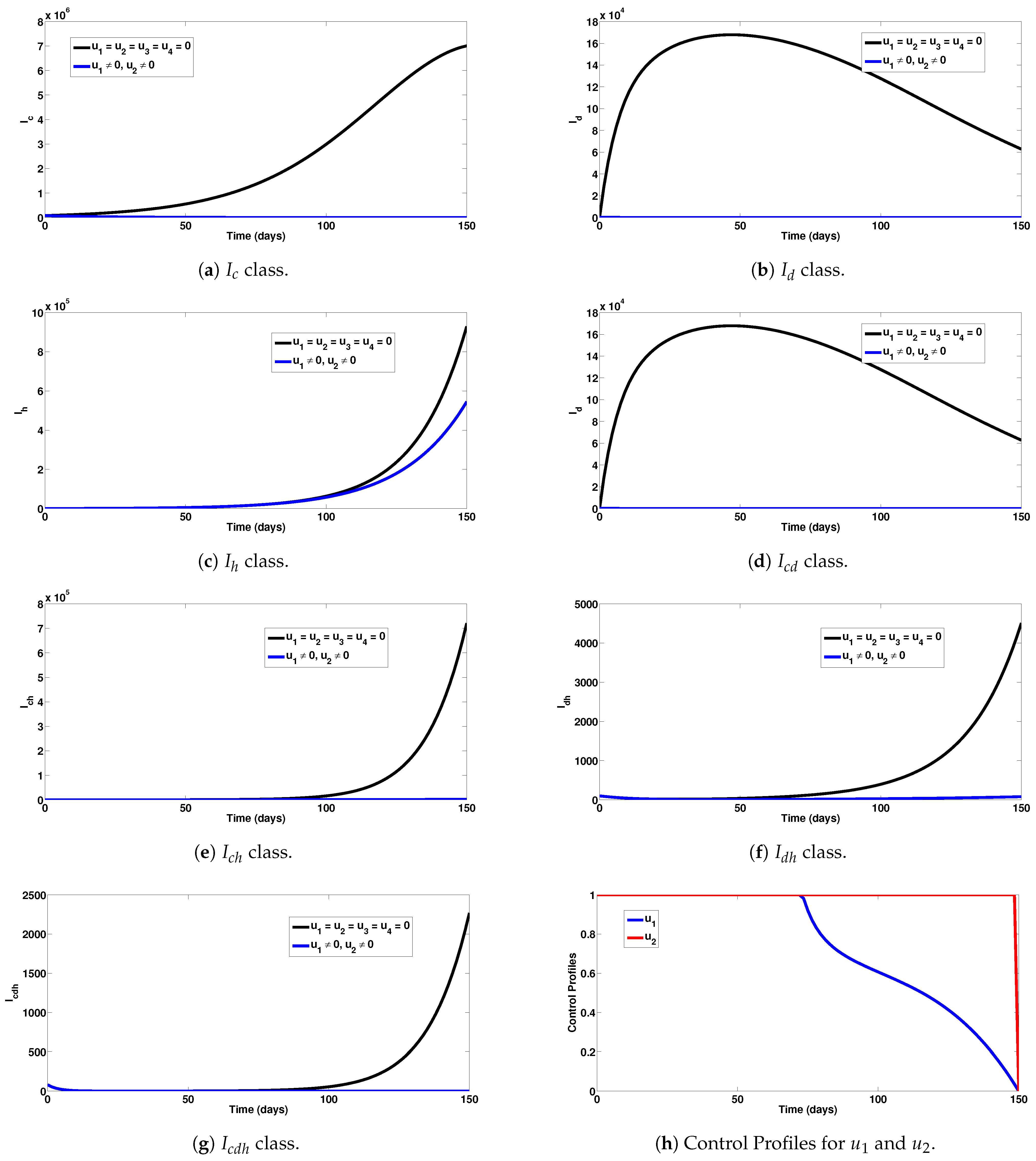
5.2. Strategy B: Assessment of COVID-19 and HIV Combined Preventive Controls ( u 1 0 , u 3 0 )

Numerical experiments to assess COVID-19 and HIV combined preventive controls when the reproduction number is given by R 0 = 2.8480 , are depicted in Figure 3a–g. It can be observed that this experimental scenario had a large positive impact on most single and co-infection cases. In particular, a total of 6,999,860 COVID-19 cases were averted under this intervention scheme (Figure 3a). The detrimental impact of this control scheme can be observed for dengue infection (Figure 3b). In addition, this intervention scheme saved 928,085 new HIV cases (Figure 3c). Co-infection cases averted were 769,235, as can be observed in Figure 3d–g. The combined single and co-infection cases prevented using this strategy were 8,697,180. The control profiles for the combined preventive efforts are given in Figure 3h. It is observed that control u 1 was at its peak for about 75 days from the onset of simulation, before decreasing gradually to zero at the final time. Similarly, control u 3 was at its peak for about 112 days, before steadily reducing to zero at the end of the simulation period. It is also interesting to note that these conclusions were reached based on the parameter values given in Table 1.

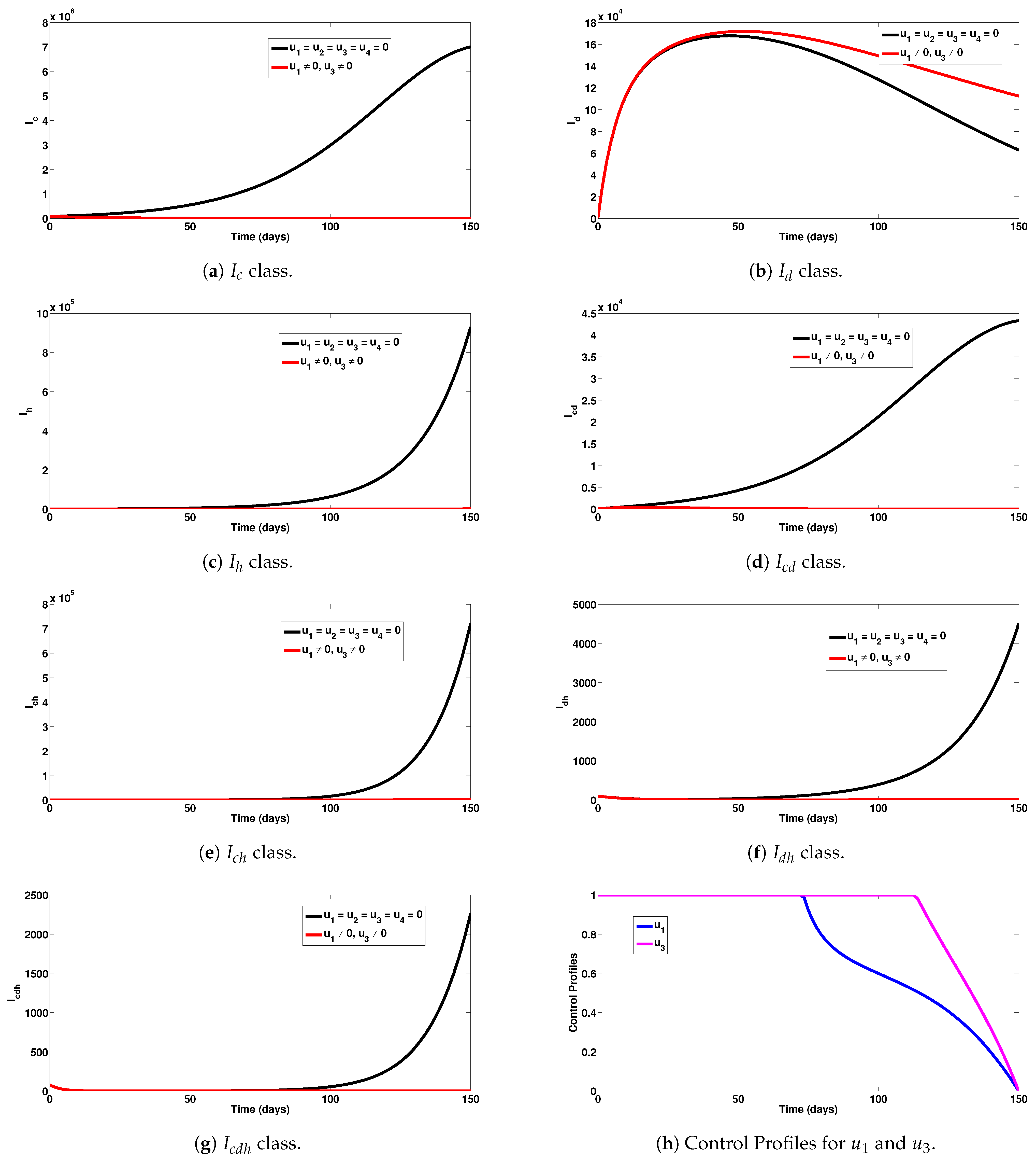
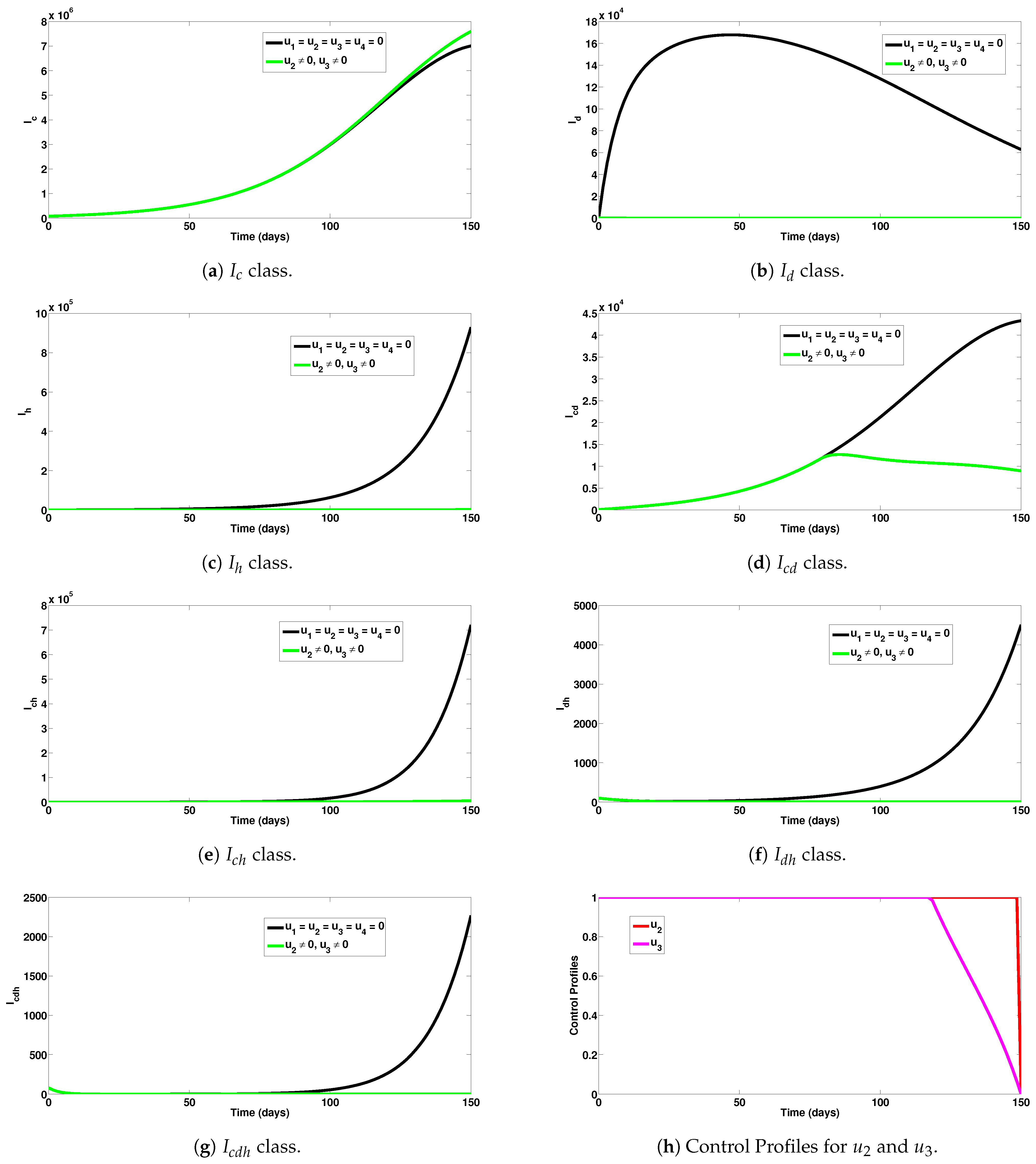
5.3. Strategy C: Assessment of COVID-19 and Co-Infection Combined Preventive Controls ( u 1 0 , u 4 0 )

Numerical experiments to assess COVID-19 and co-infection combined preventive controls when the reproduction number was given by R 0 = 2.8480 are depicted in Figure 4a–g. For instance, this intervention scheme saved a total of 6,999,843 new COVID-19 cases (as seen in Figure 4a). The detrimental impact of this control measure was observed for dengue infection (as noticed n Figure 4b). A total of 665,700 new HIV cases were also averted using this measure (as seen in Figure 4c). In addition, 770,536 co-infection cases were averted with this intervention scheme, as can be observed in Figure 4d–g. The control profiles for the combined preventive efforts are given in Figure 4h. It can be observed that control u 1 was at its peak for the first 70 days from the beginning of the simulation, while control u 4 was also at its peak value for about 87 days before gradually declining at the end of the simulation period.

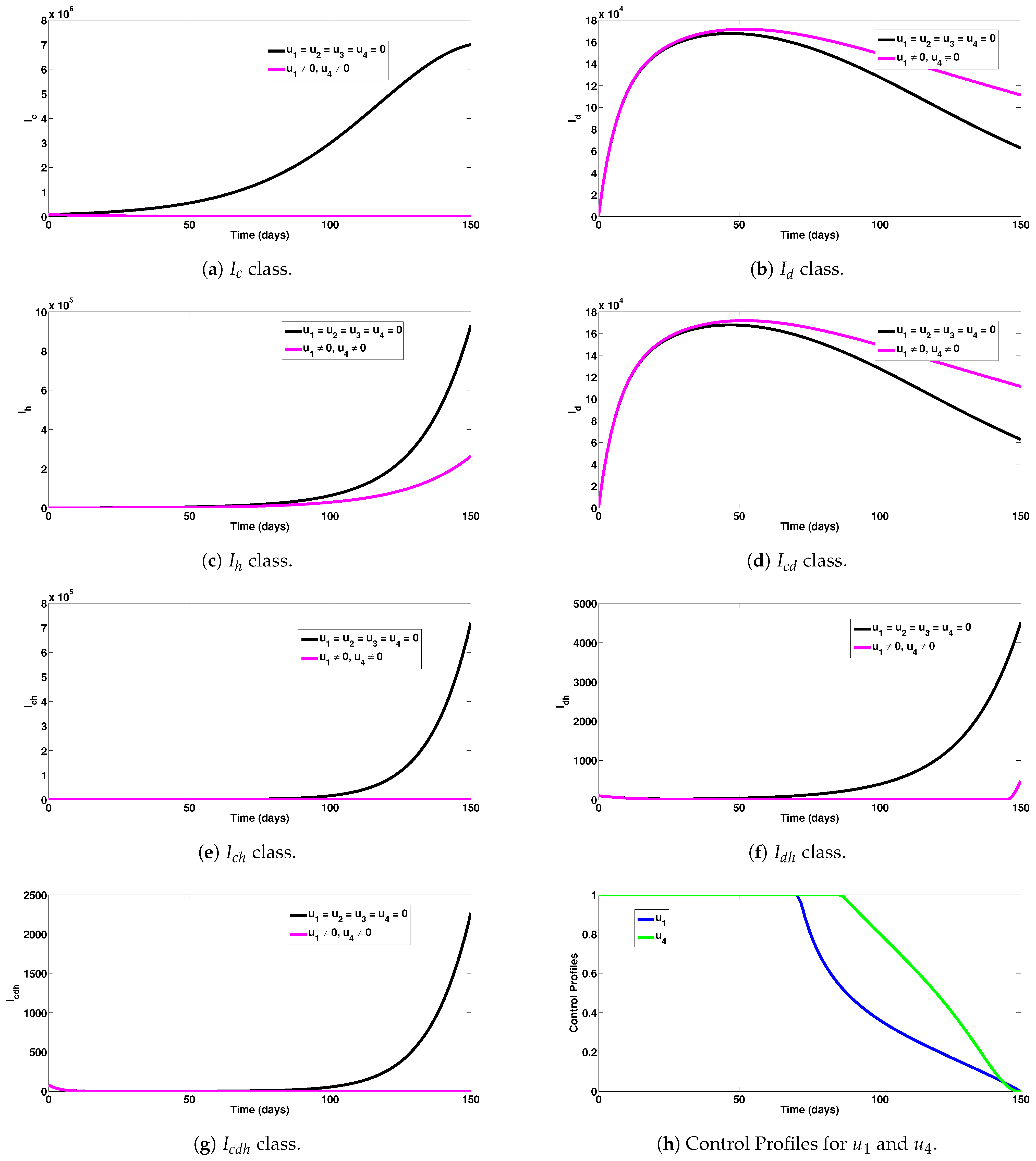
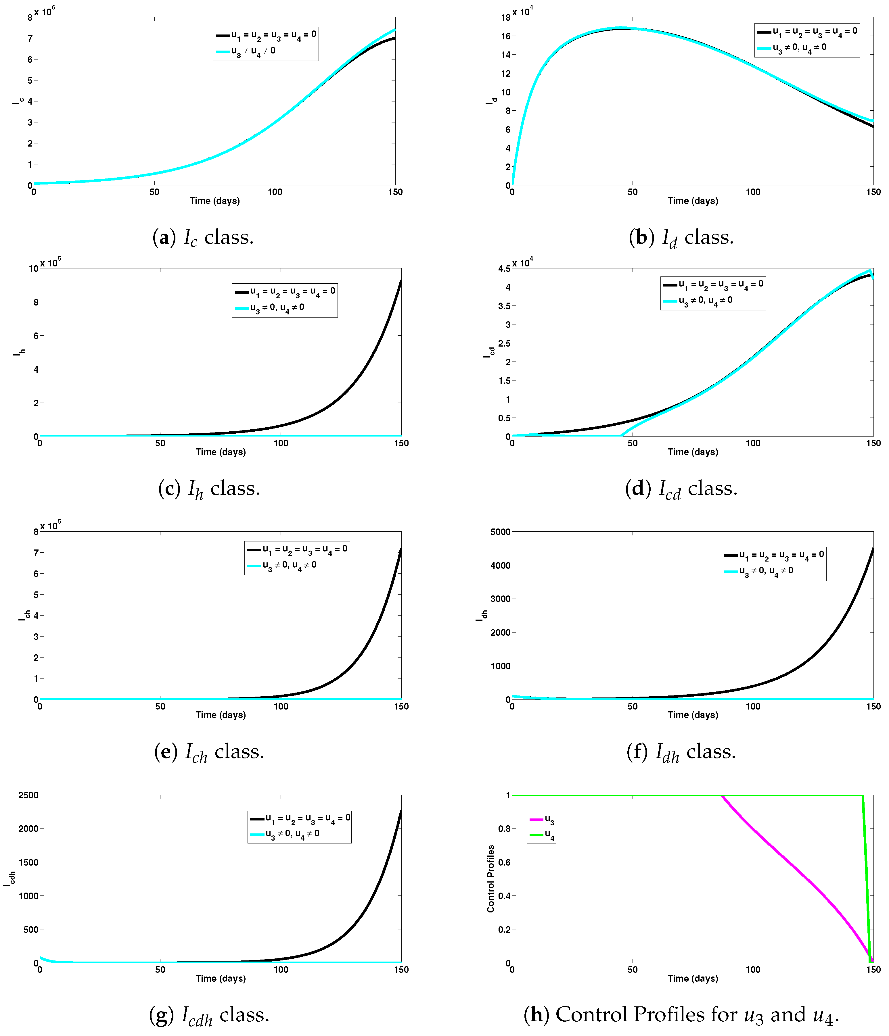
5.4. Strategy D: Assessment of Dengue and HIV Combined Preventive Controls ( u 2 0 , u 3 0 )

Numerical experiments to assess dengue and HIV combined preventive controls when the reproduction number was R 0 = 2.8480 are depicted in Figure 5a–g. In particular, this control strategy had no positive impact on COVID-19 prevention, as noticed in Figure 5a. Moreover, this intervention scheme saved a total of 62,800 new dengue and 927,381 new HIV cases, respectively, as can be seen in Figure 5b,c. A total of 757,087 co-infection cases were averted, as observed in Figure 5d–g. A total of 1,747,268 single and co-infection cases were averted using this intervention scheme. The control profiles for the combined preventive efforts of this strategy are given in Figure 5h. It can be observed that the control u 2 was at its peak for almost all of the simulation period, while the control u 2 showed the highest impact for about 118 days, before declining to zero at the final time.

5.5. Strategy E: Assessment of HIV and Co-Infection Combined Preventive Controls ( u 3 0 , u 4 0 )

Numerical experiments to assess HIV and co-infection combined preventive controls, when the reproduction number was R 0 = 2.8480 , are depicted in Figure 6a–g, respectively. It can be seen from Figure 6a,b that this intervention scheme had a marginal or detrimental impact on COVID-19 and dengue prevention. As expected, this intervention had a large impact on HIV prevention, as it averted 912,600 new HIV cases (observed in Figure 6c). The control strategy also had a marginal or detrimental impact on COVID-19 and dengue co-infection prevention (as can be noticed in Figure 6d). The control scheme averted a total of 727,252 new co-infection cases (involving HIV) (as seen in Figure 6e–g). In general, a total of 1,639,852 single and co-infection cases were averted using this intervention measure. The control profiles for the combined preventive efforts under this intervention scheme are presented in Figure 6h. It is observed that the control u 3 had a significant impact up to about 87 days, while the control u 4 , showed a large impact for about 145 days, before declining to zero at the end of the simulation period.

6. Conclusions

In this work, a new mathematical model for COVID-19, dengue, and HIV co-dynamics was proposed. Qualitative analyses to assess the dynamical behavior of the model were performed. A bifurcation analysis of the model showed that parameters accounting for re-infection and susceptibility to additional infection could cause backward bifurcation in the proposed model. For the scenario when the causes of backward bifurcation were neglected, the model’s equilibria were shown, using well-constructed Lyapunov function candidates, to be globally stable (in the asymptotic sense). To slow down the co-spread of the three infections, time-dependent intervention measures were incorporated into the model and analyzed using Pontryagin’s maximum principle. Numerical assessments of the complete co-dynamical model revealed that efforts against incident infection with each disease could reduce the burden and co-spread of all the diseases within the community. We hope to study stochastic, delayed, and agent-based versions of the modified model in future studies. Highlights of the simulations include:
(i)
Upon implementation of the first intervention strategy (control against COVID-19 and dengue), it was observed that a significant number of single and dual infection cases were averted (as can be seen in Figure 2a–g).
(ii)
Under the COVID-19 and HIV prevention strategy, a good number of new single and dual infection cases were prevented (as can be observed in Figure 3a–g).
(iii)
Under the COVID-19 and co-infection prevention strategy, a remarkable number of new infections were averted (as presented in Figure 4a–g).
(iv)
Comparing all the intervention measures considered in this study, it is concluded that the strategies combining COVID-19/HIV averted the highest number of new infections. Thus, this strategy would be the most ideal and optimal to adopt for controlling the co-spread of COVID-19, dengue, and HIV.
The findings from this study can also guide public health agencies and policy makers in developing integrated approaches for managing the co-infections of the three viral diseases. For example, targeted interventions for COVID-19, dengue, and HIV, such as increased surveillance, vaccination campaigns, and vector control measures could be implemented. In addition, by integrating data on COVID-19, dengue, and HIV cases, public health authorities could establish comprehensive surveillance systems to identify trends, hotspots, and patterns of co-infection. Early detection and timely intervention could also help prevent severe disease outcomes, reduce transmission, and improve patient outcomes. Public health authorities and policy makers could also support health education and awareness campaigns to promote knowledge about co-infections among high-risk populations and the general public. Educating individuals about the risks, symptoms, prevention, and available interventions can empower them to take appropriate action, seek timely medical care, and adopt preventive behaviors. Furthermore, by providing sufficient resources for testing, diagnosis, treatment, and supportive care for individuals with COVID-19, dengue, and HIV co-infections, the co-circulation of the three diseases can be reduced within the population and overall health outcomes improved.
This study is not without limitations. In order to avoid complications in the model, asymptomatic classes of COVID-19 and dengue were not assumed. The model also only considered the HIV infection stage, without considering the full-blown AIDS stage. In a further study, we hope to incorporate these assumptions for the purpose of capturing reality. Moreover, there is not much information available regarding vaccine or infection-acquired cross-protection between COVID-19, HIV, and dengue.No detailed clinical information yet exists as to whether the currently available COVID-19 or dengue vaccines could cross-protect against infection with HIV. We realize that a lack of detailed clinical data may have limited the accuracy and precision of the model’s predictions. Detailed clinical data, such as disease progression, symptom severity, immune responses, and co-morbidities, are important for capturing the complex interactions between COVID-19, dengue, and HIV. Future research will aim to collect and analyze comprehensive clinical data, including longitudinal studies, to better understand the interactions between the diseases and refine the model’s parameters. Therefore, with more detailed and reliable information about the co-interactions of the three diseases, further research in this direction is much desired by the authors. Further research on these viral infections’ interactions with other diseases is also anticipated, noting that mutations of diseases such as dengue and COVID-19 could occur. Thus, a model for the co-dynamics of multiple COVID-19 and dengue strains with HIV might be taken into consideration in the near future. Additionally, it was challenging to obtain proper documented records for the three viral diseases. In a subsequent investigation, we intend to fit the model to three sets of data (corresponding to the three diseases), as this will provide better and more precise estimates of the parameters. In future, the co-infection model’s findings will be validated using real-world data from diverse populations and geographical locations. By comparing the model’s predictions with observed data, researchers can assess its accuracy and reliability. Future research will also emphasize data collection from different settings and population groups, to enhance the generalizability of the model’s conclusions. Furthermore, future research will explore the effectiveness of intervention strategies, such as vaccination campaigns, antiretroviral therapy, vector control, and public health measures, within the context of co-infections. Investigating the synergistic or antagonistic effects of interventions on the three diseases could help inform the development of integrated strategies for optimal control of these three viral diseases.

Author Contributions

Conceptualization, A.O. and U.H.D.; methodology, A.O. and U.H.D.; software, A.O.; validation, A.O., A.A.R. and C.O.; formal analysis, A.O. and U.H.D.; investigation, A.O., U.H.D., A.A.R. and C.O.; data curation, A.O.; writing—original draft preparation, A.O., U.H.D., A.A.R. and C.O.; writing—review and editing, A.O., U.H.D., A.A.R. and C.O.; visualization, C.O.; supervision, A.O. and C.O.; project administration, A.O. and C.O.; funding acquisition, A.A.R. All authors have read and agreed to the published version of the manuscript.

Funding

This research was funded by the Deanship of Scientific Research at King Khalid University, KSA, Project under Grant Number RGP.2/27/44.

Data Availability Statement

Not applicable.

Acknowledgments

The authors extend their appreciation to the Deanship of Scientific Research at King Khalid University, Abha, Saudi Arabia, for funding this work through the Research Group Project under Grant Number (RGP.2/27/44).

Conflicts of Interest

The authors declare no conflict of interest.

Appendix A. Center-Manifold-Theory

Theorem A1
([47]). Consider the following system of ordinary differential equations with a parameter φ
d y d t = h ( y , φ ) , h : R n × R R and h C 2 ( R n × R ) ,
where 0 is an equilibrium point of the system (that is, h ( 0 , φ ) 0 for all φ) and assume that
(A1): 
A = D y h ( 0 , 0 ) = h i y j ( 0 , 0 ) ; linearization of system (A1) in the neighbourhood of the equilibrium 0 with φ evaluated at 0 . The matrix A has zero eigenvalue and other eigenvalues have negative real parts;
(A2): 
Matrix A has a right eigenvector ψ and a left eigenvector ϖ (each corresponding to the zero eigenvalue).
Let h k be the k t h component of h and
a = k , i , j = 1 n ϖ k ψ i ψ j 2 h k y i y j ( 0 , 0 ) , b = k , i = 1 n ϖ k ψ i 2 h k y i φ ( 0 , 0 ) .
The local dynamics of the system in the neighborhood of 0 are completely determined by the signs of a and b.
(i). 
a > 0 , b > 0 . When φ < 0 with | φ | 1 , 0 is locally asymptotically stable and there exists an unstable equilibrium; when 0 φ 1 , 0 is unstable and there exists a locally asymptotically stable equilibrium;
(ii). 
a < 0 , b < 0 . When φ < 0 with | φ | 1 , 0 is unstable; when 0 < φ 1 , 0 is locally asymptotically stable equilibrium, and there exists an unstable equilibrium;
(iii). 
a > 0 , b < 0 . When φ < 0 with | φ | 1 , 0 is unstable and there exists a locally asymptotically stable equilibrium; when 0 φ 1 , 0 is stable and an unstable equilibrium appears;
(iv). 
a < 0 , b > 0 . When φ changes from negative to positive, 0 changes its stability from stable to unstable. Correspondingly, an unstable equilibrium becomes locally asymptotically stable.
In particular, if a > 0 and b > 0 , then a backward bifurcation occurs at φ = 0 .

Appendix B. Pontryagin’s Maximum Principle

Theorem A2
([51]). Consider the optimal control problem:
max u t 0 T f ( x ( t ) , u ( t ) ) d t
subject to
x ( t ) = g ( x ( t ) , u ( t ) ) x ( t 0 ) = x 0 ,
where f : R n R n , x : [ 0 , ) R n , u : [ 0 , ) A R m and g : R n × A R .
Suppose further, that the Hamiltonian is defined by
H ( x ( t ) , u ( t ) , λ ( t ) ) = g ( x ( t ) , u ( t ) ) + i = 1 n λ i ( t ) f i ( x ( t ) , u ( t ) ) .
For the optimality of control u * ( t ) and corresponding trajectory x * ( t ) with t [ 0 , T ] , it is necessary that there exists a nonzero adjoint vector function λ * ( t ) that is a solution to the adjoint system:
λ ( t ) = H ( t , x ( t ) , u ( t ) , λ ( t ) ) x ,
λ ( T ) = 0 ,
so that the Hamiltonian
H ( x * ( t ) , u * ( t ) , λ * ( t ) ) = u U max H ( t , x * ( t ) , u ( t ) , λ * ( t ) ) .
Thus, the necessary conditions for optimizing the Hamiltonian are
H u = 0 g u + i = 1 n λ i ( t ) ( f i ) u = 0 ( optimality equation ) , λ i ( t ) = H ( x ( t ) , u ( t ) , λ ( t ) x i λ i ( t ) = g x i i = 1 n λ i ( t ) ( f i ) x i ( adjoint equation ) , λ ( T ) = 0 , transversality condition .
In addition, in a maximization problem, for each t [ 0 , T ] ,
2 H u 2 0 at u * ( t )
must hold from concavity.

References

  1. Aguiar, D.; Lobrinus, J.A.; Schibler, M.; Fracasso, T.; Lardi, C. Inside the lungs of COVID-19 disease. Int. J. Leg. Med. 2020, 134, 1271–1274. [Google Scholar] [CrossRef] [PubMed]
  2. Yang, L.; Liu, S.; Liu, J.; Zhang, Z.; Wan, X.; Huang, B.; Chen, Y.; Zhang, Y. COVID-19: Immunopathogenesis and Immunotherapeutics. Signal Transduct. Target. Ther. 2020, 5, 128. [Google Scholar] [CrossRef] [PubMed]
  3. Fernandes, Q.; Inchakalody, V.P.; Merhi, M.; Mestiri, S.; Taib, N.; Moustafa Abo El-Ella, D.; Bedhiafi, T.; Raza, A.; Al-Zaidan, L.; Mohsen, O.M.; et al. Emerging COVID-19 variants and their impact on SARS-CoV-2 diagnosis, therapeutics and vaccines. Ann. Med. 2022, 54, 524–540. [Google Scholar] [CrossRef] [PubMed]
  4. Dhama, K.; Nainu, F.; Frediansyah, A.; Yatoo, M.I.; Mohapatra, R.K.; Chakraborty, S.; Zhou, H.; Islam, M.R.; Mamada, S.S.; Kusuma, H.I.; et al. Global emerging Omicron variant of SARS-CoV-2: Impacts, challenges and strategies. J. Infect. Public Health 2022, 16, 4–14. [Google Scholar] [CrossRef]
  5. WHO. COVID-19 Webpage. 2020. Available online: https://covid19.who.int (accessed on 14 May 2023).
  6. Bosmuller, H.; Matter, M.; Fend, F.; Tzankov, A. The pulmonary pathology of COVID-19. Virchows Arch. 2021, 478, 137–150. [Google Scholar] [CrossRef]
  7. Sood, A.; Bedi, O. Histopathological and molecular links of COVID-19 with novel clinical manifestations for the management of coronavirus-like complications. Inflammopharmacology 2022, 30, 1219–1257. [Google Scholar] [CrossRef]
  8. Xu, L.; Liu, J.; Lu, M.; Yang, D.; Zheng, X. Liver injury during highly pathogenic human coronavirus infections. Liver Int. 2020, 40, 998–1004. [Google Scholar] [CrossRef]
  9. Nielsen, D.G. The relationship of interacting immunological components in dengue pathogenesis. Virol. J. 2009, 6, 211. [Google Scholar] [CrossRef]
  10. Halstead, S.B. Controversies in dengue pathogenesis. Paediatr. Int. Child Health 2012, 32 (Suppl. 1), 5–9. [Google Scholar] [CrossRef]
  11. Kok, B.H.; Lim, H.T.; Lim, C.P.; Lai, N.S.; Leow, C.Y.; Leow, C.H. Dengue virus infection? A review of Pathogenesis, Vaccines, Diagnosis and Therapy. Virus Res. 2022, 324, 199018. [Google Scholar] [CrossRef]
  12. Setiati, T.E.; Wagenaar, J.F.P.; de Kruif, M.; Mairuhu, A. Changing epidemiology of dengue haemorrhagic fever in Indonesia. Dengue Bull. 2006, 30, 1–4. [Google Scholar]
  13. Azhar, M.; Saeed, U.; Piracha, Z.Z.; Amjad, A.; Ahmed, A.; Batool, S.I.; Jabeen, M.; Fatima, A.; Noreen, F.; Uppal, R.; et al. SARS-CoV-2 related HIV, HBV, RSV, VZV, Enteric viruses, Influenza, DENV, S. Aureus TB Coinfections. Arch. Pathol. Clin. Res. 2021, 5, 26–33. [Google Scholar]
  14. WHO HIV/AIDS Webpage. Available online: https://www.who.int/news-room/fact-sheets/detail/hiv-aids (accessed on 26 May 2023).
  15. WHO HIV/AIDS Data 2021. Available online: https://www.who.int/data/gho/data/themes/hiv-aids (accessed on 26 May 2023).
  16. Hariyanto, T.I.; Rosalind, J.; Christian, K.; Kurniawan, A. Human immunodeficiency virus and mortality from coronavirus disease 2019: A systematic review and meta-analysis. South. Afr. J. HIV Med. 2021, 22, 1–7. [Google Scholar] [CrossRef] [PubMed]
  17. Spinelli, M.A.; Lynch, K.L.; Yun, C.; Glidden, D.V.; Peluso, M.J.; Henrich, T.J.; Gandhi, M.; Brown, L.B. SARS-CoV-2 seroprevalence, and IgG concentration and pseudovirus neutralising antibody titres after infection, compared by HIV status: A matched case-control observational study. Lancet HIV 2021, 8, E334–E341. [Google Scholar] [CrossRef] [PubMed]
  18. Available online: https://www.aidsmap.com/about-hiv/covid-19-and-coronavirus-people-living-hiv (accessed on 26 May 2023).
  19. Masyeni, S.; Santoso, M.S.; Widyaningsih, P.D.; Asmara, D.W.; Nainu, F.; Harapan, H.; Sasmono, R.T. Serological cross-reaction and coinfection of dengue and COVID-19 in Asia: Experience from Indonesia. Int. J. Infect. Dis. 2021, 102, 152–154. [Google Scholar] [CrossRef]
  20. COVID-19: Massive Impact on Lower-Income Countries Threatens More Disease Outbreaks Gavi, the Vaccine Alliance. 2021. Available online: https://www.gavi.org/news/media-room/covid-19-massive-impact-lower-income-countries-threatens-more-disease-outbreaks (accessed on 7 April 2022).
  21. Impact of COVID-19 on Vaccine Supplies. UNICEF Supply Division. 2020. Available online: https://www.unicef.org/supply/stories/impact-covid-19-vaccine-supplies (accessed on 7 April 2022).
  22. Darling, K.E.; Diserens, E.A.; N’garambe, C.; Ansermet-Pagot, A.; Masserey, E.; Cavassini, M.; Bodenmann, P. A cross-sectional survey of attitudes to HIV risk and rapid HIV testing among clients of sex workers in Switzerland. Sex Transm. Infect. 2012, 88, 462–464. [Google Scholar] [CrossRef]
  23. Vezzani, D.; Velazquez, S.M.; Schweigmann, N. Seasonal pattern of abundance of Aedes Aegypti (Diptera: Culicidae) Buenos Aires City, Argentina. Mem. Inst. Oswaldo Cruz 2004, 99, 351–356. [Google Scholar] [CrossRef]
  24. Pan American Health Organization; World Health Organization. PAHO, PLISA Health Information Platform for the Americas. 2019. Available online: http://www.paho.org/data/index.php/en/ (accessed on 26 April 2022).
  25. López, M.S.; Jordan, D.I.; Blatter, E.; Walker, E.; Gómez, A.A.; Müller, G.V.; Mendicino, D.; Robert, M.A.; Estallo, E.L. Dengue emergence in the temperate Argentinian province of Santa Fe, 2009–2020. Sci. Data 2021, 8, 134. [Google Scholar] [CrossRef]
  26. Khan, M.A.; Shah, S.W.; Ullah, S.; Gómez-Aguilar, J.F. A dynamical model of asymptomatic carrier zika virus with optimal control strategies. Nonlinear Anal. Real World Appl. 2019, 50, 144–170. [Google Scholar] [CrossRef]
  27. Jan, R.; Khan, M.A.; Gómez-Aguilar, J.F. Asymptomatic carriers in transmission dynamics of dengue with control interventions. Optim. Control Appl. Methods 2020, 41, 430–447. [Google Scholar] [CrossRef]
  28. Ullah, S.; Khan, M.A.; Gómez-Aguilar, J.F. Mathematical formulation of hepatitis B virus with optimal control analysis. Optim. Control Appl. Methods 2019, 40, 529–544. [Google Scholar] [CrossRef]
  29. Omame, A.; Rwezaura, H.; Diagne, M.L.; Inyama, S.C.; Tchuenche, J.M. COVID-19 and dengue co-infection in Brazil: Optimal control and cost-effectiveness analysis. Eur. Phys. J. Plus 2021, 136, 1090. [Google Scholar] [CrossRef]
  30. Hezam, I.M. COVID-19 and Chikungunya: An optimal control model with consideration of social and environmental factors. J. Ambient. Intell. Humaniz. Comput. 2022. [Google Scholar] [CrossRef] [PubMed]
  31. Omame, A.; Abbas, M.; Onyenegecha, C.P. Backward bifurcation and optimal control in a co-infection model for SARS-CoV-2 and ZIKV. Results Phys. 2022, 37, 105481. [Google Scholar] [CrossRef]
  32. Omame, A.; Okuonghae, D. A co-infection model for oncogenic Human papillomavirus and tuberculosis with optimal control and cost-effectiveness analysis. Optim. Control Appl. Methods 2021, 42, 1081–1101. [Google Scholar] [CrossRef]
  33. Bonyah, E.; Khan, M.A.; Okosun, K.O.; Gómez-Aguilar, J.F. On the co-infection of dengue fever and Zika virus. Optim. Control Appl. Methods 2019, 40, 394–421. [Google Scholar] [CrossRef]
  34. Asamoah, J.K.K.; Yankson, E.; Okyere, E.; Sun, G.-Q.; Jin, Z.; Jan, R.; Fatmawati. Optimal control and cost-effectiveness analysis for dengue fever model with asymptomatic and partial immune individuals. Results Phys. 2021, 31, 104919. [Google Scholar] [CrossRef]
  35. Ojo, M.M.; Benson, T.O.; Peter, O.J.; Goufo, E.F.D. Nonlinear optimal control strategies for a mathematical model of COVID-19 and influenza co-infection. Physica A 2022, 607, 128173. [Google Scholar] [CrossRef]
  36. Abidemi, A.; Ackora-Prah, J.; Fatoyinbo, H.O.; Asamoah, J.K.K. Lyapunov stability analysis and optimization measures for a dengue disease transmission model. Phys. A Stat. Mech. Appl. 2022, 602, 127646. [Google Scholar] [CrossRef]
  37. Bi, K.; Chen, Y.; Wu, C.-H.; Ben-Arieh, D. A memetic algorithm for solving optimal control problems of Zika virus epidemic with equilibriums and backward bifurcation analysis. Commun. Nonlinear Sci. Numer. Simul. 2020, 84, 105176. [Google Scholar] [CrossRef]
  38. Chemaitelly, H.; Nagelkerke, N.; Ayoub, H.H.; Coyle, P.; Tang, P.; Yassine, H.M.; Al-Khatib, H.A.; Smarri, M.K.; Hasan, M.R.; Al-Kanaani, Z.; et al. Duration of immune protection of SARS-CoV-2 natural infection against reinfection. J. Travel Med. 2022, 29, Taac109. [Google Scholar] [CrossRef]
  39. Salvo, C.P.; Lella, N.D.; Lopez, F.S.; Hugo, J.; Zito, J.G.; Vilela, A. Coinfection Dengue Y SARS-CoV-2 en Paciente HIV Positivo. Medicina 2020, 80, 94–96. [Google Scholar]
  40. Omame, A.; Okuonghae, D.; Nwajeri, U.K.; Onyenegecha, C.P. A fractional-order multi-vaccination model for COVID-19 with non-singular kernel. Alex. Eng. J. 2022, 61, 6089–6104. [Google Scholar] [CrossRef]
  41. Available online: https://www.indexmundi.com/argentina/demographics_profile.html (accessed on 2 December 2021).
  42. Garba, S.M.; Gumel, A.B.; Abu Bakar, M.R. Backward bifurcations in dengue transmission dynamics. Math. Biosci. 2008, 215, 11–25. [Google Scholar] [CrossRef] [PubMed]
  43. Okuneye, K.O.; Velasco-Hernandez, J.X.; Gumel, A.B. The “unholy” Chikungunya-Dengue-Zika Trinity: A Theoretical Analysis. J. Biol. Syst. 2017, 25, 545–585. [Google Scholar] [CrossRef]
  44. Omame, A.; Isah, M.E.; Abbas, M. An optimal control model for COVID-19, Zika, Dengue and Chikungunya co-dynamics with re-infection. Optim. Control Appl. Methods 2022, 44, 170–204. [Google Scholar] [CrossRef]
  45. Nwankwo, A.; Okuonghae, D. Mathematical analysis of the transmission dynamics of HIV syphilis Co-infection in the presence of treatment for syphilis. Bull. Math. Biol. 2018, 80, 437–492. [Google Scholar] [CrossRef]
  46. Van Den Driessche, P.; Watmough, J. Reproduction numbers and sub-threshold endemic equilibria for compartmental models of disease transmission. Math. Biosci. 2002, 180, 29–48. [Google Scholar] [CrossRef]
  47. Castillo-Chavez, C.; Song, B. Dynamical models of tuberculosis and their applications. Math. Biosci. Eng. 2004, 2, 361–404. [Google Scholar] [CrossRef]
  48. LaSalle, J.P. The Stability of Dynamical Systems. In Regional Conferences Series in Applied Mathematics; SIAM: Philadelphia, PA, USA, 1976. [Google Scholar]
  49. Fleming, W.H.; Rishel, R.W. Deterministic and Stochastic Optimal Control; Springer: New York, NY, USA, 1975. [Google Scholar]
  50. Rector, C.R.; Chandra, S.; Dutta, J. Principles of Optimization Theory; Narosa Publishing House: New Delhi, India, 2005. [Google Scholar]
  51. Pontryagin, L.; Boltyanskii, V.; Gamkrelidze, R.; Mishchenko, E. The Mathematical Theory of Optimal Control Process 4; John Wiley & Sons: New York, NY, USA; London, UK, 1962. [Google Scholar]
  52. Lenhart, S.; Workman, J.T. Optimal Control Applied to Biological Models; Mathematical and Computational Biology Series; Chapman &amp; Hall/CRC: Boca Raton, FL, USA, 2007. [Google Scholar]
Figure 1. Flow chart of the model (1), where, λ c = β 1 ( I c + I c d + I c h + I c d h ) N h , λ d v = β 2 h I d v N h , λ h = β 3 ( I h + I c h + I d h + I c d h ) N h , λ c h = β 13 I c h N h .
Axioms 12 00773 g001
Figure 2. Assessment of COVID-19 and dengue combined preventive controls for human epidemiological compartments. Here, β 1 = 0.2642 ; β 3 = 0.1425 ; β 13 = 0.1541 ; β 2 h = 0.7427 ; β 2 v = 0.60 , so that R 0 = max { R 0 c , R 0 d , R 0 h , R 0 c h } = 2.8480 > 1 .
Axioms 12 00773 g002
Figure 3. Assessment of COVID-19 and HIV combined preventive controls for human epidemiological compartments. Here, β 1 = 0.2642 ; β 3 = 0.1425 ; β 13 = 0.1541 ; β 2 h = 0.7427 ; β 2 v = 0.60 , so that R 0 = max { R 0 c , R 0 d , R 0 h , R 0 c h } = 2.8480 > 1 .
Axioms 12 00773 g003
Figure 4. Assessment of COVID-19 and co-infection combined preventive controls for human epidemiological compartments. Here, β 1 = 0.2642 ; β 3 = 0.1425 ; β 13 = 0.1541 ; β 2 h = 0.7427 ; β 2 v = 0.60 , so that R 0 = max { R 0 c , R 0 d , R 0 h , R 0 c h } = 2.8480 > 1 .
Axioms 12 00773 g004
Figure 5. Assessment of dengue and HIV combined preventive controls for human epidemiological compartments. Here, β 1 = 0.2642 ; β 3 = 0.1425 ; β 13 = 0.1541 ; β 2 h = 0.7427 ; β 2 v = 0.60 , so that R 0 = max { R 0 c , R 0 d , R 0 h , R 0 c h } = 2.8480 > 1 .
Axioms 12 00773 g005
Figure 6. Assessment of HIV and co-infection combined preventive controls for human epidemiological compartments. Here, β 1 = 0.2642 ; β 3 = 0.1425 ; β 13 = 0.1541 ; β 2 h = 0.7427 ; β 2 v = 0.60 , so that R 0 = max { R 0 c , R 0 d , R 0 h , R 0 c h } = 2.8480 > 1 .
Axioms 12 00773 g006
Table 1. Model parameters and description.
ParameterDescriptionValueSource
β 2 v Contact rate for human–mosquito
spread of dengue0.60–0.70 day 1 [31]
ϕ d Dengue fever induced death rate0.05 day 1 [31]
ζ c COVID-19 recovery rate 0.13978 day 1 [40]
ϕ c COVID-19-induced death rate0.015 day 1 [40]
Λ h Recruitment rate for humans 29 , 289 , 357 78.07 × 365 day 1 [41]
μ h Human natural death rate 1 78.07 × 365 day 1 [41]
Λ v Recruitment rate for mosquitoes20,000 day 1 [42]
μ v Mosquito removal rate 1 21 day 1 [42]
ζ d Dengue fever recovery rate 0.15 day 1 [43]
β 1 COVID-19 transmission rate 0.5642 day 1 [44]
β 2 h Contact rate for mosquito-human
spread of dengue0.3427 day 1 [44]
β 3 HIV transmission rate0.3425 day 1 [45]
β 13 COVID-19/HIV dual-transmission rate0.6 day 1 Assumed
ζ c d COVID-Dengue recovery rate 0.15 day 1 Assumed
ϕ h HIV induced death rate 0.3425 365 day 1 [45]
ϕ c d Co-infection death rate 0.06 day 1 Assumed
ϕ c h Co-infection death rate 0.05 day 1 Assumed
ϕ d h Co-infection death rate 0.05 day 1 Assumed
ϕ c d h Co-infection death rate 0.07 day 1 Assumed
κ Re-infection rate for COVID-19 0.7 day 1 [38]
Disclaimer/Publisher’s Note: The statements, opinions and data contained in all publications are solely those of the individual author(s) and contributor(s) and not of MDPI and/or the editor(s). MDPI and/or the editor(s) disclaim responsibility for any injury to people or property resulting from any ideas, methods, instructions or products referred to in the content.

