Article

Predictive Analytics-Based Methodology Supported by Wireless Monitoring for the Prognosis of Roller-Bearing Failure

by
Ernesto Primera
1,
Daniel Fernández
2,
Andrés Cacereño
3 and
Alvaro Rodríguez-Prieto
2,*
1
Department of Applied Statistics, University of Delaware, Newark, DE 19716, USA
2
Department of Manufacturing Engineering, Universidad Nacional de Educación a Distancia (UNED), 28040 Madrid, Spain
3
Instituto Universitario de Sistemas Inteligentes y Aplicaciones Numéricas en Ingeniería (SIANI), Universidad de Las Palmas de Gran Canaria (ULPGC), 35017 Las Palmas De Gran Canaria, Spain
*
Author to whom correspondence should be addressed.
Submission received: 6 December 2023 / Revised: 3 January 2024 / Accepted: 9 January 2024 / Published: 17 January 2024

Abstract

:
Roller mills are commonly used in the production of mining derivatives, since one of their purposes is to reduce raw materials to very small sizes and to combine them. This research evaluates the mechanical condition of a mill containing four rollers, focusing on the largest cylindrical roller bearings as the main component that causes equipment failure. The objective of this work is to make a prognosis of when the overall vibrations would reach the maximum level allowed (2.5 IPS pk), thus enabling planned replacements, and achieving the maximum possible useful life in operation, without incurring unscheduled corrective maintenance and unexpected plant shutdown. Wireless sensors were used to capture vibration data and the ARIMA (Auto-Regressive Integrated Moving Average) and Holt–Winters methods were applied to forecast vibration behavior in the short term. Finally, the results demonstrate that the Holt–Winters model outperforms the ARIMA model in precision, allowing a 3-month prognosis without exceeding the established vibration limit.

1. Introduction

Prognostics and health monitoring (PHM) analysis requires several stages, including data collection, data processing, condition monitoring, diagnostics, prognostics, and decision support [1]. The information generated by a PHM system can be divided into diagnostics and prognostics. Diagnostics include anomaly detection, fault isolation, fault classification, and uncertainty [2], while prognostics include the estimation of the remaining useful life (RUL) and the prediction of behavior at the design stage. These procedures ensure that the component is in good condition before installation and operation.
Researchers have identified the importance of information on the system’s operational condition [3,4,5]. The selection of the appropriate technology for data acquisition, as well as the extraction and management of these data, has been a challenge, as can be seen in several reports, such as the Forbes survey by Gil Press [6], where preparing and managing data for analysis took around 80% of the research time.
Rolling bearings are some of the most crucial components in rotating machinery systems; therefore, their failure may cause substantial economic losses and even endanger operators’ lives [7]. An interesting background report about rolling bearings covering topics such as, their historical development, characteristics, types or selection, and dimensioning depending on the application, was provided by Desnica et al. [8]. Rolling-bearing faults represent up to 51% of all rotating mechanical problems, making them one of the main factors affecting the reliable and safe operation of mechanical systems [9,10]. The identification of the root cause of the bearing failure becomes very complex due to the combination of several factors, such as the misalignment of the ball bearing fitted in the main shaft of an aero engine, as described by Ejaz et al. [11], or the misalignment in the angular contact ball bearing, as investigated by Murugesan et al. [12]. Other examples of bearing failures can originate from undesirable electrical currents between the track surfaces for races [13] or improper assembly operation, such as the use of excessive tightening force, as reported by Hou et al. [14]. All these cases reveal the importance of monitoring the health status of bearings during operation to reduce equipment failure [15].
It is very important to take into account that the cost of each bearing is approximately USD 200k, and the labor needed to replace the bearing costs USD 150k, incurring a total cost of approximately USD 350k per bearing to keep the bearings serviced. Hence, to prevent unexpected shutdowns, it is necessary to plan these activities to avoid penalty costs for non-compliance with the production plan and secondary effects on other equipment in the process. Therefore, the prediction of an accurate remaining useful life (RUL) of this type of component is key to optimizing maintenance/replacement tasks and improving the efficiency of machine operation. The methodology for prediction of RUL has two phases: data collection and health indicator (HI) definition. HI construction is the process of reflecting the bearing degradation from data; therefore, the construction of HI directly affects the accuracy of RUL prediction. Furthermore, it allows maintenance to be scheduled in advance while ensuring a fault-free service life [16]. Several authors have studied prognostic modeling options for RUL, such as knowledge-based options, life expectancy, and artificial networks, as described by Sikorska et al. [17]; data-driven models (DDMs) [18,19], physics-based models (PbMs) [20,21], or both, as shown by Cubillo et al. [22]; a signal-level deep learning framework as proposed by Wang et al. [23]; computer modeling and simulation, as studied by Andraș et al. [24]; the use of auto-associative kernel regression, as proposed by Baraldi et al. [25]; a method that includes monitoring bearing degeneration, determining the initial degeneration point, and RUL estimation, based on combining a novel health indicator and particle filtering, as proposed by Quiu et al. [26]; a combination of machine learning techniques, such as a regression model and multilayer artificial neural network model, as explored by Li et al. [27]; an investigation of the time-dependent reliability of the main shaft device based on the accumulation of fatigue damage, as performed by Cao et al. [28]; and an artificial neural network model provided by Patil et al. [29] to measure the wear of several ball bearing materials.
Bearings are commonly employed in numerous engineering applications, such as power plants [30], machines for production lines [31], aerospace applications [32], marine applications [33], railway vehicles [34,35], wind turbines [36], robotic applications [37], and mining applications [38]. Some of the techniques employed for bearing diagnostics are acoustic emissions [39] and thermal analysis [40]. As the analysis of vibration signals is a widely used technique, there are several studies on this topic, such as the one performed by Ali et al. [41], which proposed a method based on run-to-failure vibration signals using an artificial neural network. Bertoni and André [42] proposed a bearing diagnosis method called the Bearing Frequency Estimation Method to detect the early appearance of bearing faults. Shakya et al. [43] proposed a Time Synchronous Averaging method that uses data from probes in close proximity to supplement the information from the accelerometer. This approach improved the accuracy of bearing diagnosis. Kass et al. [44] developed an indicator to detect, identify, and classify faults on rolling elements. This indicator is based on the Fast-Order-Frequency Spectral Coherence. Its capability for self-running diagnosis has been demonstrated. Kecik et al. [45] evaluated the effectiveness of the recurrence method for detecting defects in ball bearings and demonstrated its promising performance in short time series.
This work focuses on the use of wireless sensors to collect data and vibration signal-processing-based approaches, which present some advantages. Statistical features, such as the root mean square (RMS) [46], are suitable degradation indicators for predicting bearing defects and their sizes [47,48].
The Holt–Winters and ARIMA (Auto-Regressive Integrated Moving Average) models for univariate time series are analyzed and compared to confirm which one is the most reliable for prediction. The prognosis of univariate time series represents a great challenge for predictive analytics models since the most robust models are multivariate and include predictor variables, such as multiple regression, Support Vector Machine (SVM) [49], and the COX model. Thus, this research aims to provide a methodology, applying advanced analytical techniques (adequate for univariate time series), such as the Holt–Winters and ARIMA models, to establish reliable predictions of vibration behavior based on experimental data obtained from wireless monitoring to plan maintenance activities and visualize a mechanical condition pattern of the rollers that allows their useful life to be increased.

2. Materials and Methods

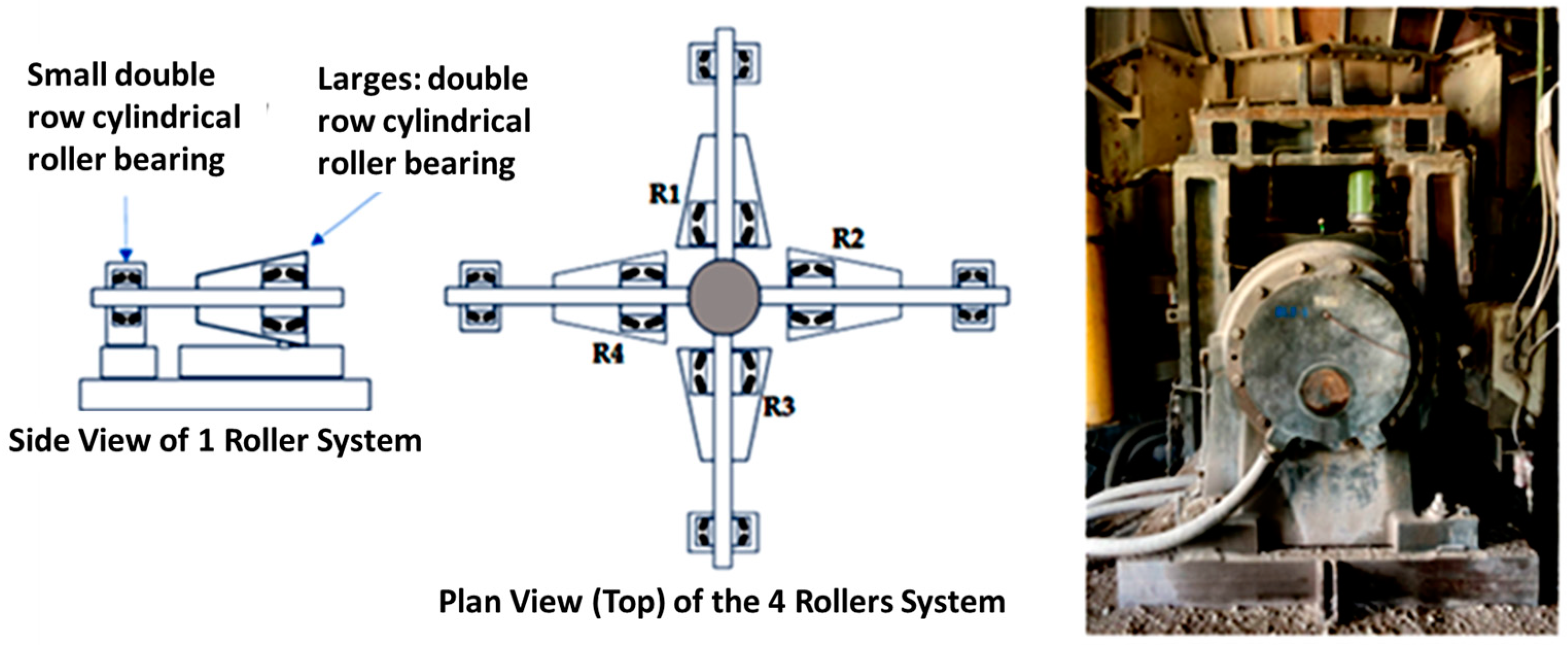
2.1. Geometrical Dimensions, Set-Up, and Process Parameters

For this research, a four-shaft centric roller mill from a cement production plant was used to set up the roller system in which two double-row spherical roller bearings (designation F-562181.02.PRL) were installed in each of the four shafts.
The bearings were of different sizes; the larger one received the greatest amount of operating load, and was also subjected to vertical damping movements, as shown in Figure 1.
The main features of the equipment are shown in Table 1. Figure 2 shows the section of the roller bearing.
The vibration data-collection technology selected was a biaxial piezoelectric accelerometer wireless sensor (technical specifications in Table 2) to capture vibration data within the frequency range of 0.5 Hz to 5000 Hz, together with the Sensor-Agnostic Condition Monitoring Software Platform by © SensOs v. 2023.
These sensors were installed on the four rollers as required, as shown in Figure 3.
The characteristics of the captured data are summarized as follows:
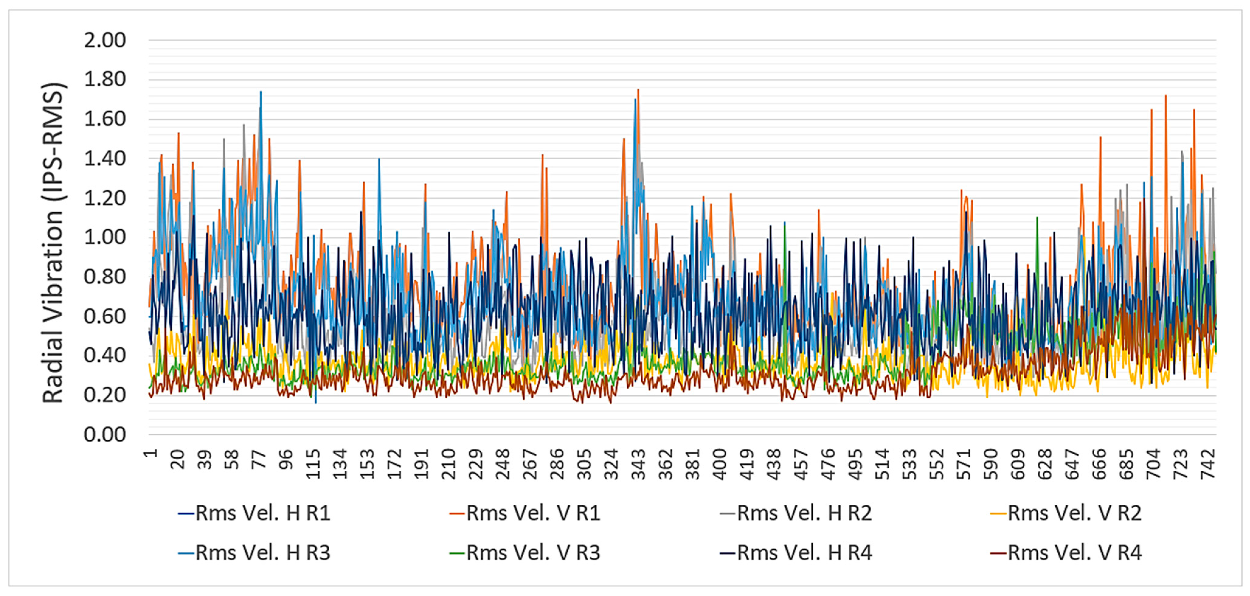
  • Four rollers were analyzed, classified as R1, R2, R3, and R4.
  • Vibrations were measured in RMS velocity (IPS) and acceleration (g’s).
  • Vibrations were captured in the radial horizontal (H) and vertical (V) directions.
  • Data were captured every 5 min with Spectrums and Waveforms.
  • The capture period was 25 June to 25 October of 2021 (Timeframe).
Figure 4 provides the trends of the overall vibration of the 4 rollers during the period observed.

2.2. Data Modeling

For the effective analysis of data, the selection of suitable analytic methodologies is vital. In this study, the data were modeled utilizing both the CRISP-DM (The Cross-Industry Standard Process for Data Mining) [50] and SEMMA (Sample, Explore, Modify, Model, and Assess) [51,52] methodologies. In the CRISP-DM’s modeling phase, mathematical techniques were employed to formulate models, be they equations or other logic, to bolster business decision making [53]. During the SEMMA modeling phase, emphasis was placed on employing various data-mining techniques on the prepared data, striving to establish models that potentially yield the anticipated outcome [17]. Descriptive analytics, involving data aggregation and data mining, offers insights into past events, answering the question, “What has happened?”. Meanwhile, predictive analytics employ statistical models and forecasting techniques to offer a perspective on potential future events, addressing the query, “What could happen?” [22]. For this model phase, data mining and statistical software SAS® Studio, together with R Studio statistical computing software, were used.
Descriptive analysis was conducted to pinpoint the current severity levels of the rollers and set the permitted thresholds. This analysis encompassed:
  • A descriptive statistical examination of time series data;
  • The inspection of extreme values.
Models aiming to predict time series variables, or for prognosis, strive to forecast a variable’s future behavior based on its historical behavior. Identifying suitable models for time series data is a complex task. A strategy akin to that devised by Box and Jenkins in 1976 involves three primary steps [54]:
  • Model identification;
  • Model fitting;
  • Model diagnostics.

2.3. Predictive Models

Predictive analytics were used in this study to evaluate two widely recognized methods for univariate time series modeling: ARIMA (Auto-Regressive Integrated Moving Average) and Holt–Winters (exponential smoothing), both implemented in R code.

2.3.1. ARIMA

This model is expressed as ARIMA (p, d, q), where (AR) is auto-regressive, (I) is the integration, (MA) is the moving average, (p) is an auto-regressive term that denotes the number of auto-regressive orders, (d) specifies the order of differentiation applied to the series to the estimate model, and (q) specifies the order of moving average parts [55]. Some advantages of using ARIMA are that it:
  • Is good for short-term forecasting;
  • Only needs historical data;
  • Models non-stationary data.
However, there are certain constraints to be considered before applying the ARIMA method, such as computation weakness due to the integration and moving average part of the model. The parameters p, d, and q need to be manually defined. In addition, this model cannot be applied in cases where there is multiple seasonality.
This method is time-series-based and depends on the assumption that the series is stationary. Therefore, the first step of the process is to check whether the assumption is fulfilled using the Dickey–Fuller (DF) stationary test [56]. This test consists of proving the null hypothesis that there is a unit root in an AR model, which implies that the data series is not stationary.
The model-selection test using PACF (Partial Auto Correlation Function) [57] provides the model’s orders, such as p for AR and q for MA, to select the best model for forecasting. This function is part of the Box–Jenkins approach to time series modeling.
Finally, the Box–Ljung test (often called the “portmanteau” test) is applied to evaluate the model. This test is based on the autocorrelation plot, but instead of testing randomness at each distinct lag, it tests the “overall” randomness based on the number of lags.
The formula for the ARIMA model in R is given in Equation (1):
X t = a 1 X t 1 + + a p X t p + e t + b 1 e t 1 + + b k e t k
where
-
Xt is the time series value at time t;
-
a1, , ap are the parameters of the autoregressive part of the model;
-
et is the error term at time t;
-
b1, , bk are the parameters of the moving average part of the model.

2.3.2. Holt–Winters

The Holt–Winters model, also known as triple exponential smoothing, is used for forecasting time series data when there is a trend and seasonal pattern. Exponential smoothing encompasses various methods. The most elementary form is termed simple exponential smoothing, which is pertinent to series without a pronounced trend or seasonality. For series with a trend but lacking seasonality, Holt’s method is suitable. Should there be seasonality, potentially accompanied by a trend, Winters’ method becomes relevant. It must be pointed out that this method assumes that the level, trend, and seasonality of the data have to be constant or linear; otherwise, it is not very reliable for complex and nonlinear patterns. Notably, the latter two methods are often jointly referred to as the Holt–Winters model [58].
The formula for the additive version of the model in R is shown in Equation (2):
Y t + h ^ = a t + h b t + s [ t p + 1 + ( h 1 ) mod   p ]
where:
  • Y t + h ^ = the forecast equation;
  • at = the level component;
  • bt = the trend component;
  • st = the seasonal component;
  • p = the length of the seasonal period;
  • h = the number of periods ahead for forecasting.
The level component (at) is obtained using Equation (3):
at = α ∗ (Ytstp) + (1 – α) ∗ (at1 + bt1)
The trend component (bt) is calculated using Equation (4):
bt = β ∗ (at − at1) + (1 − β) ∗ bt1
Finally, Equation (5) is used to obtain the seasonal component (st):
st = γ ∗ (Ytat) + (1 − γ) ∗ stp
The three aspects of the time series behavior—value, trend, and seasonality—are expressed as three types of exponential smoothing. The model requires the parameters (α, β, γ).
Smoothing parameters:
α (alpha) = smoothing parameter for the level, the “base value”. A higher alpha puts more weight on the most recent observations.
β (beta) = smoothing parameter for the trend, the “trend value”. A higher beta means the trend slope is more dependent on recent trend slopes.
γ (gamma) = smoothing parameter for the seasonal component, the “seasonal component”. A higher gamma puts more weight on the most recent seasonal cycles.

2.3.3. Models Comparison

After applying the ARIMA and Holt–Winters models, it is necessary to compare the two models to determine which model should be utilized for each roller. The criteria used to select the most effective model included comparisons of the two models’ mean error (ME) and mean absolute percentage error (MAPE) [59]. Additionally, the mean absolute error (MAE) and root mean squared error (RMSE) for each model were analyzed to determine the effectiveness of each model. Percentage errors are useful because they are scale-independent and can compare forecasts between different data series.
The MAE and RMSE are scale-dependent errors that can be used to evaluate the individual models and can be used as comparisons between data series that are on the same scale. The formulas for the evaluation measures are shown in Equations (6)–(8):
R M S E = 1 n i = 1 n ( a i c i ) 2
M A E = a 1 + c 1 + a 2 + c 2 + + a n + c n n
M A P E = 1 n i = 1 n a i c i a i
where:
  • ai = predicted values;
  • ci = observed values;
  • n = number of observations.

3. Results and Discussion

3.1. Data Collection and Analysis

Utilizing the comprehensive vibration data, each model projected daily radial vibrations from 25 June 2021 to 25 October 2021. Given the limited number of variables in the datasets, no variables were excluded during the modeling process, as each had a significant impact on the accuracy of the predictive model.
Multiple models were crafted and evaluated utilizing various software packages and open-source languages, including SPSS (Statistical Package for the Social Sciences) [60] and SAS (Statistical Analysis System) [61].
The descriptive analytics presented in Table 3 encompass a comprehensive summary of the vibration values for each roller, exhibiting a Gaussian distribution. This pattern suggests that the behavior of the overall vibration values is predictable and can be extrapolated for further analysis and forecasting.
The severity chart was constructed using the overall vibration mean values and the sum of the accumulated overall vibrations, which is named the exposure time to high vibrations. As a result, a clear correlation appeared that shows that Roller #1 and Roller #3 had the highest level of overall vibrations and the greatest time of exposure, as shown in Figure 5.
For the analysis of extreme values, only values greater than Inch/S (IPS) were captured.
As shown in Figure 6, it can be clearly seen that Roller #1 and Roller #3 were the most exposed to extreme values; the severity shown in Figure 5 is thereby validated.

3.2. ARIMA Model Application

To apply the ARIMA methodolody, it is first necessary to check whether the series are stationary. Therefore, as explained in Section 2.3.1., the Dickey–Fuller test was applied, whose results are shown in Table 4.
From the stationary tests, it can be observed that the p-value obtained (0.01) is lower than the theoretical p-value of 0.05; therefore, the alternative hypothesis is accepted, and it is concluded that the series is stationary.
The next step is to perform a model selection test by using PACF in accordance with the Box–Jenkins approach; see Table 5.
Figure 7 shows the forecast from ARIMA (1,1,1) and ARIMA (3,1,1) with the drift for Roller #1 and Roller #3, respectively.
The model evaluation from the Box–Ljung test showed a good fit to the data from both Rollers R1 and R3, since the p-values are greater than 0.05, and there is white noise. Therefore, the model successfully addresses the underlying project goal, which is to predict the rollers’ overall vibration. Moreover, the Average Absolute Percentage Error is 15.39% for Roller R1 and 4.85% for Roller R3, as shown in Table 6.

3.3. Holt–Winters Model Application

The parameters set during the vibration model’s creation ensured the consideration of non-seasonality and the inclusion of diverse model types for optimal forecast accuracy. The Holt–Winters exponential smoothing parameter values for value, trend, and seasonality are shown in Table 7.
In Figure 8, it can be seen that using the Holt–Winters command in R [62] creates a graph in red, where a new series of data is created that are in theory very close to the original data, which are in black.
Figure 8 shows the vibration time series data for Rollers #1 and #3, comparing the Holt–Winters model’s training set (black) and test set (red):
Roller #1: The training set data, depicted in black, show fluctuations around a mean level with no clear trend. The test set data, in red, appear to follow the training set pattern quite closely, suggesting that the model has captured the underlying process well for the training period.
Roller #3: Similar to Roller #1, the black line, representing the training set data, shows variability around a central level. The test set data, in red, also track the training data closely, indicating a good fit of the model to the observed data for the time period considered.
In both cases, the close tracking of the test data to the training data suggests that the Holt–Winters model performs adequately in forecasting the vibration levels for both rollers.
Figure 9 shows the results of Holt–Winters filtering for vibration data of rollers R1 and R3.
The black line represents the observed vibration data.
The red line indicates the fitted values from the Holt–Winters model, which shows the model’s attempt to capture the underlying trend and seasonality up to the last historical point.
The blue line forecasts future vibration values based on the model’s fitted values.
The vertical dotted line marks the boundary between historical data and forecasted values.
For Roller #1, the forecast suggests a steady increase in vibration levels, while for Roller #3, a decline is predicted. Both forecasts show a divergence from the relatively stable historical pattern, which could be indicative of changing conditions or potential issues requiring attention.

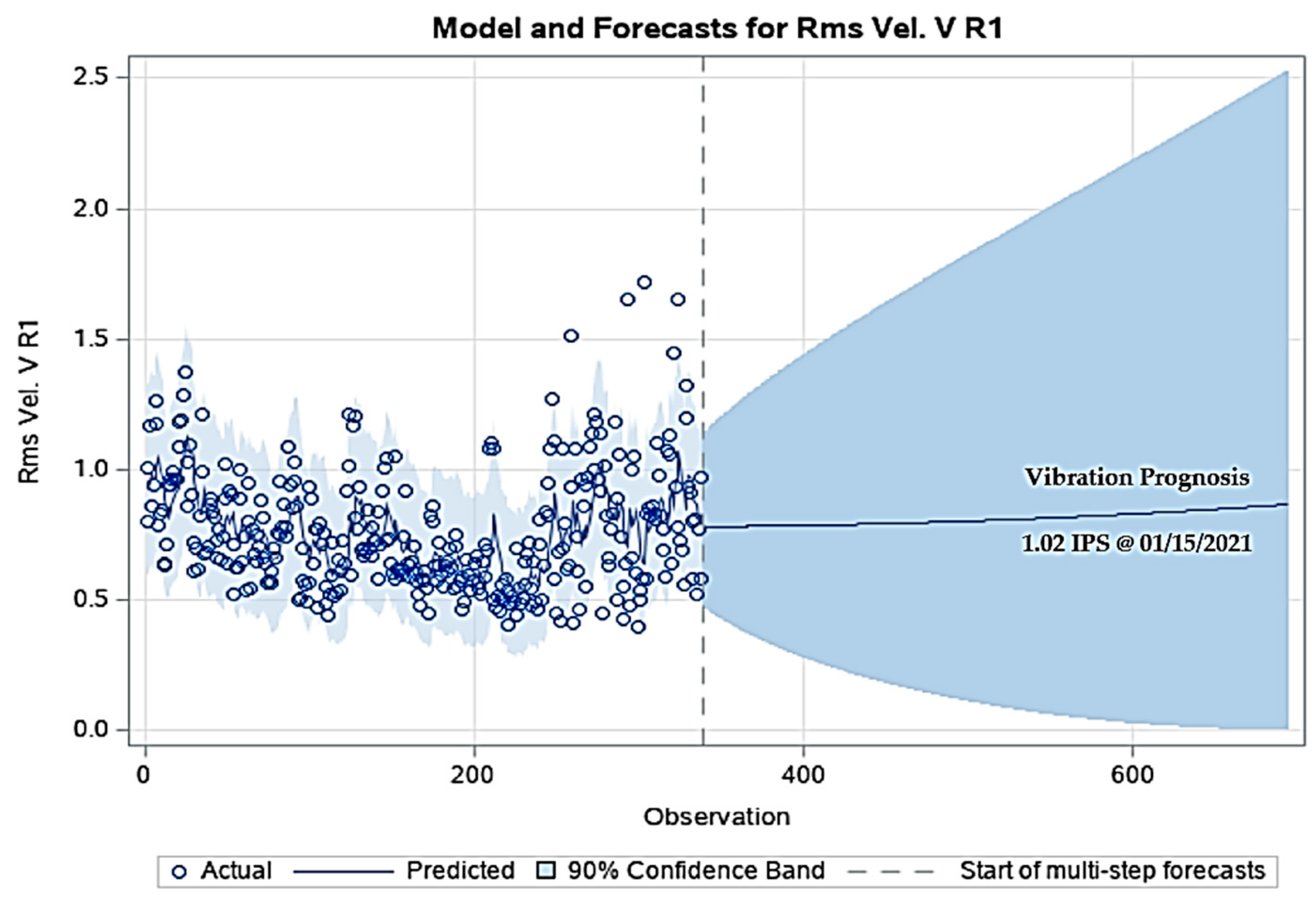
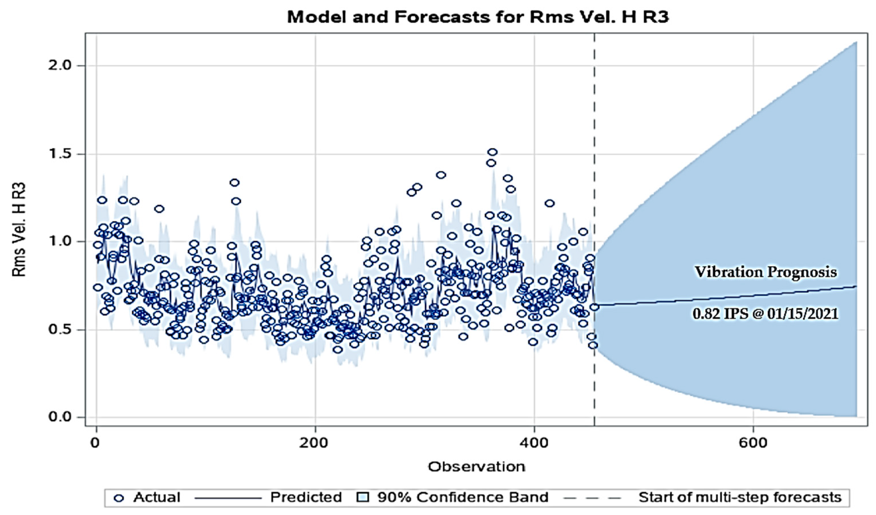
3.4. Model Comparison and Prognosis

Table 8 indicates that the Holt–Winters model outperforms the ARIMA model for both rollers’ data sets, with lower MAPE, MAE, and RMSE. Although both models show acceptable accuracy when compared, the Holt–Winters method was the best fit, so it was selected for prognosis.
The evaluation period was approximately 4 months, and a prognosis of 3 months was made for both rollers in R [63], and 4 months with SAS, with a confidence interval of 90%.
In R, the prognosis for Roller #1 shows a stable and linear trend with a slight positive slope; however, the uncertainty level exceeds 2.5 IPS at 2 months, but in SAS, the prognosis confidence band raises the limit of 2.5 IPS at 4 months, as can be seen in Figure 10. Taking this factor into account and based on the confidence interval, it can be concluded that the model is accurate for a 3-month prognosis without the risk that vibrations may exceed the unacceptable limit of 2.5 IPS.
Projecting until 15 January 2022, the vibration value will be at an average of 1.02 IPS, as shown in Figure 10.
In R, the prognosis for Roller #3 shows a stable and linear trend with a positive slope; however, the uncertainty level exceeds 2.5 IPS at 2 months, but in SAS, the prognosis confidence band raises the limit of 2.5 IPS at 3 months (see Figure 11). Thus, the situation is very similar to that for Roller #1; therefore, it can be concluded that the model is accurate for a 2.5-month prognosis without the risk that vibrations may exceed the unacceptable limit of 2.5 IPS.
Figure 11 shows that, for a projection until 15 January 2022, the vibration value will average 0.82 IPS.

4. Conclusions

This research was motivated by the need for innovation in the traditional predictive maintenance methods. The application of statistical methods such as Holt–Winters and ARIMA, which allow for better results to be achieved and the operational life of key industrial components to be extended, ultimately contributes to more efficient and economical plant operations. In order to do this, the mechanical condition of a four-roller mill was evaluated, focusing on the largest cylindrical roller bearings, which are known to be the predominant failure point in such equipment. Utilizing wireless sensors, we captured vibration data across a broad frequency range for four months, aiming to predict when overall vibrations would attain critical levels. Severity analysis underscored Rollers #1 and #3 as bearing the majority of the overall vibrations, which was corroborated by analyses of exposure time and extreme values. The ARIMA and Holt–Winters forecasting methods, adept for short-term prediction in such univariate time series, were implemented and compared, with the result that the Holt–Winters outperformed ARIMA in precision. The study progressed through established PHM stages, culminating in a prognostic model that reliably forecasts vibration trends without signaling imminent bearing failure within the next three months, allowing for timely maintenance scheduling and thus, averting unscheduled downtime.
The research culminates with the recommendation for quarterly model updates to leverage accumulating data for enhanced accuracy. It highlights the necessity for advanced statistical expertise to interpret complex models and suggests integrating expert insights for outlier management.
Finally, this study contributes to the ongoing research on rotating equipment failure prognosis, focusing on univariate models in this specific case. Future investigations will progress toward the implementation of multivariate models.

Author Contributions

Conceptualization, E.P. and A.R.-P.; methodology, E.P.; formal analysis, E.P. and A.R.-P.; investigation, E.P. and A.R.-P.; resources, A.R.-P.; writing—original draft preparation, E.P.; writing—review and editing, D.F., A.C., and A.R.-P.; supervision, A.R.-P.; project administration, A.R.-P.; funding acquisition, A.R.-P. All authors have read and agreed to the published version of the manuscript.

Funding

This work has been funded by the project 2021V/-TAJOV/006 from the Santander-UNED Call for Research Projects named “Young Talents 2021” and has been developed in the framework of the activities of Research Group of the UNED “Industrial Production and Manufacturing Engineering (IPME)” and the Industrial Research Group “Advanced Failure Prognosis for Engineering Applications”.

Data Availability Statement

The raw/processed data required to reproduce these findings cannot be shared at this time, as the data also form part of an ongoing study.

Acknowledgments

Authors want to thank Michael Bryant (Retired Accenture Endowed Professor at University of Texas at Austin and Founder and CEO of Machine Essence Corporation) for his valuable recommendations related to this research work.

Conflicts of Interest

The authors declare no conflicts of interest.

Abbreviations

The following abbreviations and symbols are used in this manuscript:
AICAkaike Information Criterion
AICcCorrected Akaike Information Criterion
ARIMAAuto-Regressive Integrated Moving Average
CRISP-DMCross-Industry Standard Process for Data Mining
DDMsData-Driven Models
DFDickey–Fuller
HIHealth Indicator
MAEMean Absolute Error
MAPEMean Absolute Percentage Error
MEMean Error
PACFPartial Auto Correlation Function
PHMPrognosis and Health Monitoring
RMSRoot Mean Square
RMSERoot Mean Square Error
RULRemaining Useful Life
SASStatistical Analysis System
SEMMASample, Explore, Modify, Model, and Assess
SPSSStatistical Package for the Social Sciences
SVMSupport Vector Machine

References

  1. Chapman, P.; Clinton, J.; Kerber, R.; Khabaza, T.; Reinartz, T.; Shearer, C.; Wirth, R. CRISP-DM Step-by-Step Data Mining Guide; SPSS: Chicago, IL, USA, 2000. [Google Scholar]
  2. Soualhi, A.; Lamraoui, M.; Elyousfi, B.; Razik, H. PHM SURVEY: Implementation of Prognostic Methods for Monitoring Industrial Systems. Energies 2022, 15, 6909. [Google Scholar] [CrossRef]
  3. Zio, E. Reliability engineering: Old problems and new challenges. Reliab. Eng. Syst. Saf. 2009, 94, 125–141. [Google Scholar] [CrossRef]
  4. Chen, B.; Chen, Z.; Chen, F.; Xiao, W.; Xiao, N.; Fu, W.; Li, G. Reliability Assessment Method Based on Condition Information by Using Improved Proportional Covariate Model. Machines 2022, 10, 337. [Google Scholar] [CrossRef]
  5. Ghodrati, B.; Hoseinie, S.H.; Kumar, U. Context-driven mean residual life estimation of mining machinery. Int. J. Min. Reclam. Environ. 2018, 32, 486–494. [Google Scholar] [CrossRef]
  6. Press, G. Cleaning Big Data: Most Time-Consuming, Least Enjoyable Data Science Task, Survey Says; Forbes Publications: Charleston, SC, USA, 2016; Available online: https://www.forbes.com/sites/gilpress/2016/03/23/data-preparation-most-time-consuming-least-enjoyable-data-science-task-survey-says/ (accessed on 8 August 2023).
  7. Ye, Z.; Zhang, Q.; Shao, S.; Niu, T.; Zhao, Y. Rolling Bearing Health Indicator Extraction and RUL Prediction Based on Multi-Scale Convolutional Autoencoder. Appl. Sci. 2022, 12, 5747. [Google Scholar] [CrossRef]
  8. Desnica, E.; Ašonja, A.; Radovanović, L.; Palinkaš, I.; Kiss, I. Selection, Dimensioning and Maintenance of Roller Bearings. In Lecture Notes in Networks and Systems, Proceedings of the 31st International Conference on Organization and Technology of Maintenance (OTO 2022), Osijek, Croatia, 12 December 2022; Blažević, D., Ademović, N., Barić, T., Cumin, J., Desnica, E., Eds.; Springer: Cham, Switzerland, 2023; Volume 592. [Google Scholar] [CrossRef]
  9. Manjurul Islam, M.M.; Kim, J.-M. Reliable multiple combined fault diagnosis of bearings using heterogeneous feature models and multiclass support vector Machines. Reliab. Eng. Syst. Saf. 2019, 184, 55–66. [Google Scholar] [CrossRef]
  10. Peng, B.; Bi, Y.; Xue, B.; Zhang, M.; Wan, S. A Survey on Fault Diagnosis of Rolling Bearings. Algorithms 2022, 15, 347. [Google Scholar] [CrossRef]
  11. Ejaz, N.; Salam, I.; Tauqir, A. Failure Analysis of an Aero Engine Ball Bearing. J. Fail. Anal. Prev. 2006, 6, 25–31. [Google Scholar] [CrossRef]
  12. Murugesan, V.; Sreejith, P.S.; Sundaresan, P.B.; Ramasubramanian, V. Analysis of an Angular Contact Ball Bearing Failure and Strategies for Failure Prevention. J. Fail. Anal. Prev. 2018, 18, 471–485. [Google Scholar] [CrossRef]
  13. Prashad, H. Diagnosis of Rolling-Element Bearings Failure by Localized Electrical Current Between Track Surfaces of Races and Rolling-Elements. J. Tribol. 2002, 124, 468–473. [Google Scholar] [CrossRef]
  14. Hou, X.; Diao, Q.; Liu, Y.; Liu, C.; Zhang, Z.; Tao, C. Failure Analysis of a Cylindrical Roller Bearing Caused by Excessive Tightening Axial Force. Machines 2022, 10, 322. [Google Scholar] [CrossRef]
  15. Lee, J.; Wu, F.; Zhao, W.; Ghaffari, M.; Liao, L.; Siegel, D. Prognostics and health management design for rotary machinery systems—Reviews, methodology and applications. Mech. Syst. Signal. Process. 2014, 42, 314–334. [Google Scholar] [CrossRef]
  16. Lim, C.; Kim, S.; Seo, Y.-H.; Choi, J.-H. Feature extraction for bearing prognostics using weighted correlation of fault frequencies over cycles. Struct. Health Monit. 2020, 19, 1808–1820. [Google Scholar] [CrossRef]
  17. Sikorska, J.Z.; Hodkiewicz, M.; Ma, L. Prognostic modelling options for remaining useful life estimation by industry. Mech. Syst. Signal Process. 2011, 25, 1803–1836. [Google Scholar] [CrossRef]
  18. Jouin, M.; Gouriveau, R.; Hissel, D.; P’era, M.-C.; Zerhouni, N. Degradations analysis and aging modeling for health assessment and prognostics of PEMFC. Reliab. Eng. Syst. Saf. 2016, 148, 78–95. [Google Scholar] [CrossRef]
  19. Ali, J.B.; Brigitte, C.M.; Lotfi, S. Accurate bearing remaining confidence interval of reliability with three-parameter Weibull distribution and artificial neural network. Mech. Syst. Signal Process. 2015, 56–57, 150–172. [Google Scholar]
  20. Zeming, L.; Jianmin, G.; Hongquan, J. A maintenance support framework based on dynamic reliability and remaining useful life. Measurement 2019, 147, 106835. [Google Scholar] [CrossRef]
  21. Tse, Y.L.; Cholette, M.E.; Tse, P.W. A multi-sensor approach to remaining useful life estimation for a slurry pump. Measurement 2019, 139, 140–151. [Google Scholar] [CrossRef]
  22. Cubillo, A.; Perinpanayagam, S.; Esperon-Miguez, M. A review of physics-based models in prognostics: Application to gears and bearings of rotating machinery. Adv. Mech. Eng. 2016, 8, 1–21. [Google Scholar] [CrossRef]
  23. Wang, T.; Li, X.; Wang, W.; Du, J.; Yang, X. A spatiotemporal feature learning-based RUL estimation method for predictive maintenance. Measurement 2023, 214, 112824. [Google Scholar] [CrossRef]
  24. Andraș, A.; Radu, S.M.; Brînaș, I.; Popescu, F.D.; Budilică, D.I.; Korozsi, E.B. Prediction of Material Failure Time for a Bucket Wheel Excavator Boom Using Computer Simulation. Materials 2021, 14, 7897. [Google Scholar] [CrossRef] [PubMed]
  25. Baraldi, P.; Bonfanti, G.; Zio, E. Differential evolution-based multi-objective optimization for the definition of a health indicator for fault diagnostics and prognostics. Mech. Syst. Signal Process. 2018, 102, 382–400. [Google Scholar] [CrossRef]
  26. Qiu, M.; Li, W.; Jiang, F.; Zhu, Z. Remaining Useful Life Estimation for Rolling Bearing with SIOS-Based Indicator and Particle Filtering. IEEE Access 2018, 6, 24521–24532. [Google Scholar] [CrossRef]
  27. Li, X.; Elasha, F.; Shanbr, S.; Mba, D. Remaining Useful Life Prediction of Rolling Element Bearings Using Supervised Machine Learning. Energies 2019, 12, 2705. [Google Scholar] [CrossRef]
  28. Cao, S.; Chen, G.; Peng, Y.; Lu, H.; Ren, F. Uncertainty analysis and time-dependent reliability estimation for the main shaft device of a mine hoist. Mech. Based Des. Struct. Mach. 2022, 50, 2221–2236. [Google Scholar] [CrossRef]
  29. Patil, A.A.; Desai, S.S.; Patil, L.N.; Patil, S.A. Adopting artificial neural network for wear investigation of ball bearing materials under pure sliding condition. Appl. Eng. Lett. 2022, 7, 81–88. [Google Scholar] [CrossRef]
  30. Jakubek, B.; Grochalski, K.; Rukat, W.; Sokol, H. Thermovision measurements of rolling bearings. Measurement 2022, 189, 110512. [Google Scholar] [CrossRef]
  31. Stack, J.R.; Habetler, T.G.; Harley, R.G. Fault classification and fault signature production for rolling element bearings in electric machines. IEEE Trans. Ind. Appl. 2004, 40, 735–739. [Google Scholar] [CrossRef]
  32. Rejith, R.; Kesavan, D.; Chakravarthy, P.; Narayana Murty, S.V.S. Bearings for aerospace applications. Tribol. Int. 2023, 181, 108312. [Google Scholar] [CrossRef]
  33. Marey, N.A.; Ali, A.A. Novel measurement and control system of universal journal bearing test rig for marine applications. Alex. Eng. J. 2023, 73, 11–26. [Google Scholar] [CrossRef]
  34. Huang, Y.; Lin, J.; Liu, Z.; Wu, W. A modified scale-space guiding variational mode decomposition for high-speed railway bearing fault diagnosis. J. Sound Vib. 2019, 444, 216–234. [Google Scholar] [CrossRef]
  35. Ulbricht, A.; Zeidler, F.; Bilkenroth, F.; Soltysiak, S. Structural lightweight components for energy-efficient rail vehicles using high performance composite materials. Transp. Res. Procedia 2023, 72, 1685–1692. [Google Scholar] [CrossRef]
  36. Dhanola, A.; Garg, H.C. Tribological challenges and advancements in wind turbine bearings: A review. Eng. Fail. Anal. 2020, 118, 104885. [Google Scholar] [CrossRef]
  37. He, Y.; Zhao, C.; Zhou, X.; Shen, W. MJAR: A novel joint generalization-based diagnosis method for industrial robots with compound faults. Robot. Comput.-Integr. Manuf. 2024, 86, 102668. [Google Scholar] [CrossRef]
  38. Mitrovic, R.M.; Miskovic, Z.Z.; Djukic, M.B.; Bakic, G.M. Statistical correlation between vibration characteristics, surface temperatures and service life of rolling bearings—Artificially contaminated by open pit coal mine debris particles. Procedia Struct. Integr. 2016, 2, 2338–2346. [Google Scholar] [CrossRef]
  39. Ghamd, A.M.; Mba, D.H. A comparative experimental study on the use of acoustic emission and vibration analysis for bearing defect identification and estimation of defect size. Mech. Syst. Signal Process. 2006, 20, 1537–1571. [Google Scholar] [CrossRef]
  40. Takabi, J.; Khonsari, M.M. Experimental testing and thermal analysis of ball bearings. Tribol. Int. 2013, 60, 93–103. [Google Scholar] [CrossRef]
  41. Ali, J.B.; Fnaiech, N.; Saidi, L.; Chebel-Morello, B.; Fnaiech, F. Application of empirical mode decomposition and artificial neural network for automatic bearing fault diagnosis based on vibration signals. Appl. Acoust. 2015, 89, 16–27. [Google Scholar]
  42. Bertoni, R.; André, H. Proposition of a bearing diagnosis method applied to IAS and vibration signals: The Bearing Frequency Estimation Method. Mech. Syst. Signal Process. 2023, 187, 109891. [Google Scholar] [CrossRef]
  43. Shakya, P.; Darpe, A.K.; Kulkarni, M.S. Bearing diagnosis using proximity probe and accelerometer. Measurement 2016, 80, 190–200. [Google Scholar] [CrossRef]
  44. Kass, S.; Raad, A.; Antoni, J. Self-running bearing diagnosis based on scalar indicator using fast order frequency spectral coherence. Measurement 2019, 138, 467–484. [Google Scholar] [CrossRef]
  45. Kecik, K.; Smagala, A.; Ciecieląg, K. Diagnosis of angular contact ball bearing defects based on recurrence diagrams and quantification analysis of vibration signals. Measurement 2023, 216, 112963. [Google Scholar] [CrossRef]
  46. Minescu, M.; Marius, S. Fault Detection and Analysis at Pumping Units by Vibration Interpreting Encountered in Extraction of Oil. J. Balk. Tribol. Assoc. 2015, 21, 711–723. [Google Scholar]
  47. Saruhan, H.; Sandemir, S.; Çiçek, A.; Uygur, I. Vibration Analysis of Rolling Element Bearings Defects. J. Appl. Res. Technol. 2014, 12, 384–395. [Google Scholar] [CrossRef]
  48. Salem, A.; Abdelrahman, A.; Sassi, S.; Renno, J. Time-Domain Based Qualification of Surface Degradation for Better Monitoring of the Health Condition of Ball Bearings. Vibration 2018, 1, 172–191. [Google Scholar] [CrossRef]
  49. Chen, X.; Shen, Z.; He, Z.; Sun, C.; Liu, Z. Remaining Life Prognostics of Rolling Bearing Based on Relative Features and Multivariable Support Vector Machine. Proc. Inst. Mech. Eng. Part C J. Mech. Eng. Sci. 2013, 227, 2849–2860. [Google Scholar] [CrossRef]
  50. Shearer, C. The CRISP-DM model: The New Blueprint for Data Mining. J. Data Warehous. 2000, 5, 13–22. [Google Scholar]
  51. Rohanizadeh, S.S.; Moghadam, M.B. A Proposed Data Mining Methodology and its Application to Industrial Procedures. J. Optim. Ind. Eng. 2010, 1, 37–50. [Google Scholar]
  52. Matignon, R. Data Mining Using SAS Enterprise MinerTM; John Wiley and Sons: Hoboken, NJ, USA, 2007. [Google Scholar]
  53. Mao, L.; Davies, B.; Jackson, L. Application of the sensor selection approach in polymer electrolyte membrane fuel cell prognostics and health management. Energies 2017, 10, 1511. [Google Scholar] [CrossRef]
  54. Albright, S.C. Business Analytics: Data Analysis and Decision Making; Cengage Learning: Boston, MA, USA, 2017. [Google Scholar]
  55. Alshawarbeh, E.; Abdulrahman, A.T.; Hussam, E. Statistical Modeling of High Frequency Datasets Using the ARIMA-ANN Hybrid. Mathematics 2023, 11, 4594. [Google Scholar] [CrossRef]
  56. Rybak, A.; Rybak, A.; Kolev, S.D. Modeling the Photovoltaic Power Generation in Poland in the Light of PEP2040: An Application of Multiple Regression. Energies 2023, 16, 7476. [Google Scholar] [CrossRef]
  57. Zuhdi, F.; Anggraini, R.S.; Yusuf, R. Rubber Production Projection in Riau Province Using Autoregressive Integrated Moving Average (ARIMA) Approach. J. Econ. 2022, 18, 40–50. [Google Scholar] [CrossRef]
  58. Nurhamidah, N.; Nusyirwan, N.; Faisol, A. Forecasting Seasonal Time Series Data using the Holt-Winters Exponential Smoothing Method of Additive Models. J. Mat. Integr. 2020, 16, 151–157. [Google Scholar] [CrossRef]
  59. Hyndman, R.J.; Koehler, A.B. Another look at measures of forecast accuracy. Int. J. Forecast. 2006, 22, 679–688. [Google Scholar] [CrossRef]
  60. Moreno, E. Manual de Uso de SPSS, 1st ed.; Universidad Nacional de Educación a Distancia: Madrid, Spain, 2008. [Google Scholar]
  61. Der, G.; Everitt, B.S. Analyses Using SAS, 3rd ed.; CRC Press Taylor & Francis Group: Boca Raton, FL, USA, 2008. [Google Scholar]
  62. Wickham, H.; Çetinkaya-Rundel, M.; Grolemund, G. R for Data Science, 2nd ed.; O’Reilly Media: Sebastopol, CA, USA, 2023. [Google Scholar]
  63. Cowpertwait, P.S.P.; Metcalfe, A.V. Introductory Time Series with R; Springer: New York, NY, USA, 2009. [Google Scholar]
Figure 1. Mill roller bearings set up.
Machines 12 00069 g001
Figure 2. Sectional drawing of roller bearings with bearing detail.
Machines 12 00069 g002
Figure 3. Locations of wireless sensors in mill roller bearings.
Machines 12 00069 g003
Figure 4. Overall vibration trends of the roller bearings.
Machines 12 00069 g004
Figure 5. Overall vibration trend of each roller.
Machines 12 00069 g005
Figure 6. Analysis of extreme values of the overall vibrations: (a) Roller #1, (b) Roller #2, (c) Roller #3, and (d) Roller #4.
Machines 12 00069 g006
Figure 7. R1 and R3 ARIMA Vibration Time Series 2-month forecasting. NOTE: The blue line represents the projection of the vibrations, and the blue and gray area is the confidence limit of the projection, which is 95%.
Machines 12 00069 g007
Figure 8. Vibration time series data for R1 and R3 for the Holt–Winters training set (black) vs. the test set (red).
Machines 12 00069 g008
Figure 9. Holt–Winters filtering for vibration time series for R1 and R3 with 3-month forecasting.
Machines 12 00069 g009
Figure 10. Holt–Winters vibration time series prognosis for R1.
Machines 12 00069 g010
Figure 11. Holt–Winters vibration time series prognosis for R3.
Machines 12 00069 g011
Table 1. General bearing weight and dimensions.
Roller Weight (kg)Roller Weight (lb)Outside Diameter (cm)Outside Diameter (in)
17593878109043
Table 2. Technical specifications of wireless sensors.
Type of CharacteristicDescription
Sensor FeaturesIP 67 Rated/3.6 V Battery/weight: 100 g/Size: 47 mm × 33 mm.
Mounting typeUniversal Heavy-duty Magnet
Gateway typeCloud connectivity, Modbus TCP/IP communication, MQTT protocol, and OPC communication
Gateway featureConventional 5 VDC at 2 A power supply/Processor Quad Core 105 GHz/RAM 512 Mb/Wi-Fi protocol 2.4 and 5 GHz
Table 3. Summary of overall vibration.
Statistical ParameterRms Vel. H
Roller #1
Rms Vel. H
Roller #2
Rms Vel. H
Roller #3
Rms Vel. H
Roller #4
Mean0.7480.6170.6930.616
Variance0.0600.0640.0460.033
Std. Dev.0.2450.2520.2150.183
Median0.6900.5600.6600.610
Mode0.1920.1860.1670.148
Minimum0.6000.5700.5200.890
Maximum0.3500.2500.0400.265
Count748.000748.000748.000748.000
Sum559.710461.700518.500461.115
Table 4. Summary of the Dickey–Fuller test results.
Stationary TestR1R3
Dickey–Fuller−5.0492−5.3859
Lag order67
p-value0.010.01
Alternative hypothesisstationarystationary
Table 5. Summary of model selection test results.
Model Selection Test
Suggested by PACFAR(1)AR(3)
ModelARIMA(1,1,1)ARIMA(3,1,1)
SeriesR1R3
Drift Coefficients
 ar10.23990.2974
0.06080.0511
 ar2-0.0434
-0.0510
 ar3-0.1078
-0.0510
 ma1−0.9327−0.9327
0.02500.0250
 drift−3 × 10⁻⁴−3 × 10⁻⁴
1 × 10−31 × 10−3
σ2 estimation0.043320.0296
log likelihood51.48156.22
AIC94.96300.44
AICc94.84300.26
Table 6. Summary of the Box–Ljung test.
Model Evaluation (Box–Ljung Test)
dataResiduals (Roller #1)Residuals (Roller #3)
X-squared0.0715790.0013889
df11
p-value0.78910.9703
Table 7. Summary of the Holt–Winters test’s parameters’ results.
Stationary TestR1R3
α (alpha)0.30.2
β (beta)0.10.1
γ (gamma)0.10.1
level0.950.95
Table 8. Performance evaluation of the methods.
Roller #1 Overall VibrationMEMAPEMAERMSE
ARIMA−0.079 0.212 0.088 15.394
Holt–Winters−0.050 0.1970.08514.210
Roller #3 Overall VibrationMEMAPEMAERMSE
ARIMA−0.007 0.138 0.055 7.850
Holt–Winters−0.006 0.100 0.0364.850
Disclaimer/Publisher’s Note: The statements, opinions and data contained in all publications are solely those of the individual author(s) and contributor(s) and not of MDPI and/or the editor(s). MDPI and/or the editor(s) disclaim responsibility for any injury to people or property resulting from any ideas, methods, instructions or products referred to in the content.

