Article

A Numerical Study on Roughness-Induced Adhesion Enhancement in a Sphere with an Axisymmetric Sinusoidal Waviness Using Lennard–Jones Interaction Law

by
Antonio Papangelo
1,2,* and
Michele Ciavarella
1,2
1
Politecnico di BARI, Department of Mechanics, Mathematics and Management, Via Orabona 4, 70126 Bari, Italy
2
Department of Mechanical Engineering, Hamburg University of Technology, Am Schwarzenberg-Campus 1, 21073 Hamburg, Germany
*
Author to whom correspondence should be addressed.
Submission received: 3 August 2020 / Revised: 2 September 2020 / Accepted: 3 September 2020 / Published: 4 September 2020
(This article belongs to the Special Issue Interfacial Dissipative Phenomena in Tribomechanical Systems)

Abstract

:
Usually, roughness destroys adhesion and this is one of the reasons why the “adhesion paradox”, i.e., a “sticky Universe”, is not real. However, at least with some special type of roughness, there is even the case of adhesion enhancement, as it was shown clearly by Guduru, who considered the contact between a sphere and a wavy axisymmetric single scale roughness, in the limit of short-range adhesion (JKR limit). Here, the Guduru’s problem is numerically solved by using the Boundary Element Method (BEM) with Lennard–Jones interaction law, which allowed us to explore the contact solution from the rigid to the JKR limit. It is shown that adhesion enhancement stops either for low Tabor parameter, or by large waviness amplitudes, due to the appearance of internal cracks within the contact patch. We do not seem to find a clear threshold for “stickiness” (complete elimination of adhesion), contrary to other recent theories on random roughness. The enhancement effect is well captured by an equation in terms of the Johnson parameter derived by Ciavarella–Kesari–Lew, and is much larger than the Persson–Tosatti enhancement in terms of increase of real contact area due to roughness. The Persson–Tosatti energetic argument for adhesion reduction seems to give a lower bound to the effective work of adhesion.

Graphical Abstract

1. Introduction

Adhesion is a challenging topic in tribology [1,2,3] with relevance in several engineering applications that range from biomimetics [4], soft matters [5], soft robots [6], grippers [7], friction [8,9,10,11,12]. Although roughness is usually responsible for adhesion reduction [13,14,15], Briggs and Briscoe [16] showed already in 1977 that relatively small random roughness amplitude could enhance adhesion in pull-off experiments as well as relative rolling resistance by a factor up to 2.5. Later, Guduru [17] showed that in the contact between a rigid sphere and a soft halfspace with an axisymmetric single wavelength waviness, adhesion could be enhanced by a factor up to 20 with respect to the Johnson–Kendall–Roberts smooth case ([18], JKR in the following). The enhancement was first modeled theoretically by Guduru [17] and then proved experimentally by Guduru and Bull [19]. The basic assumptions of the Guduru [17] model are that (i) the contact area is simply connected (there are no circular grooves within the contact patch) and that (ii) the halfspace is constituted by a soft material (elastomer or rubber) hence adhesion can be simply modeled by JKR theory [18]. Loading and unloading a rigid sphere from the wavy surface leads to several jump instabilities and related dissipation, which is responsible for the measured enhancement. Kesari et al. [20] showed that if the roughness wavelength is substantially shorter than the sphere radius, then an envelope solution can be obtained, which describes well the loading-unloading hysteretical behavior well known to experimentalists (see also Kesari and Lew [21]).
Waters and coauthors in [22] developed a Maugis–Dugdale cohesive model, still based on the assumption of simply connected contact area, to account for the transition between the rigid and JKR limit. They showed that toughening and strengthening of the interface was mostly restricted to the JKR regime, while, in the rigid limit, they found the Bradley [23] solution for the smooth rigid sphere. Ciavarella [24] further discussed the assumptions of the Guduru model and the conclusions of Waters and coauthors [22]. In particular he noticed that for hard solids (i.e., in the rigid limit) the axisymmetric roughness should reduce the macroscopic adhesion by orders of magnitude with respect to the smooth sphere limit. Ciavarella [24] supported his argument by considering the Rumpf–Rabinowich model ([25,26,27]), which geometry is analogous but not equal to that of Guduru and is used for adhesion of hard particles (the model neglects the elastic deformation). The Rumpf–Rabinowich model predicts that increasing the substrate roughness the macroscopic adhesion force first decreases and then increases again. Ciavarella [24] suggested that the Guduru and the Rumpf–Rabinowich models may be respectively close to an upper and a lower bound for macroscopic adhesion of rough bodies (see also Ciavarella [28]).
In this paper, we reconsider the geometry of Guduru [17] and obtain a closed form solution for the rigid limit, which clearly shows that increasing the waviness amplitude A reduces the macroscopic adhesion force by orders of magnitude. By using the axisymmetric Boundary Element Method (BEM) the contact problem is solved with Lennard–Jones interaction law, for varying waviness amplitude A and wavelength λ and for different Tabor parameters of the sphere μ , without the restrictive assumption of a compact contact area. Numerical results are well in agreement with the theory both in the rigid and in the JKR limit. The transition from one regime to the other is numerically studied using the BEM code. In the JKR regime adhesion enhancement is well captured by the Johnson parameter as derived by Ciavarella–Kesari–Lew [21,24], and is much larger than the Persson–Tosatti enhancement [13] in terms of increase of real contact area due to roughness. It is shown that at large Tabor parameters μ > 3 , increasing A first leads to adhesion enhancement as predicted by Guduru theory [17], but then strongly reduces the macroscopic adhesive force due to the appearance of internal cracks. We found that for A / λ 10 1 the JKR solution greatly overestimates the pull-off force and the hysteretical dissipation.

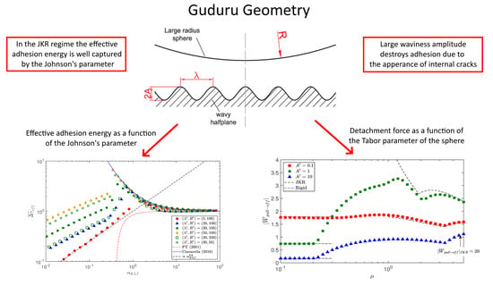
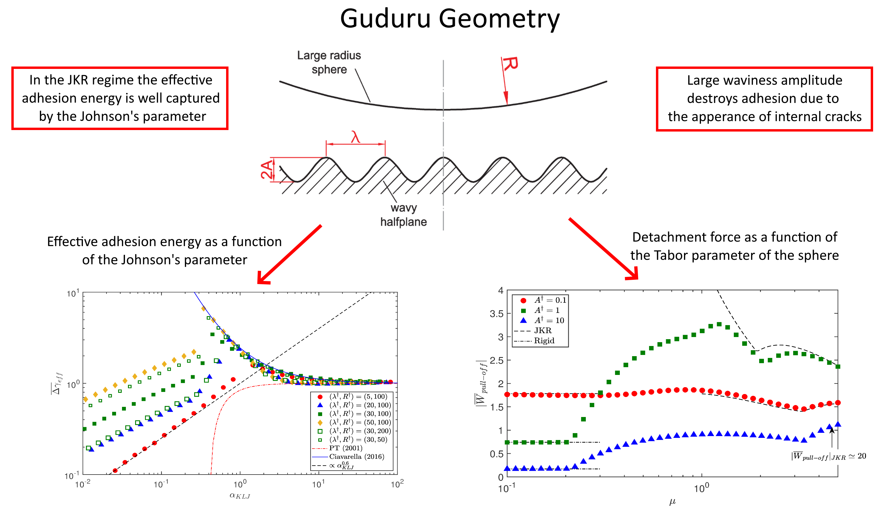
2. Guduru Contact Problem

JKR Theory

Guduru [17] considered the contact between a rigid sphere of radius R that indents and elastic halfspace (Young modulus E, Poisson ratio ν ) with an axisymmetric waviness of wavelength λ and amplitude A (see Figure 1).
In the system of reference shown in Figure 1, the axisymmetric waviness has the form
y ( r ) = A 1 cos 2 π r λ
where r is the radial coordinate. Using the Hertzian approximation for the spherical profile [29] one gets the gap function
f r = r 2 2 R + A 1 cos 2 π r λ
Guduru [17] solved the adhesive contact problem under the assumptions of compact contact area (i.e., there are no axisymmetric grooves within the contact patch) and in the limit of short range adhesion [18], which requires soft bodies into contact with large surface energy. Ensuring the contact area is compact requires that the gap function is strictly monotonically increasing
d f ( r ) d r > 0 , r > 0
which for the gap function (2) implies
λ 2 A R > 8.5761
Nevertheless, condition (4) is too restrictive. Indeed, Guduru [17] analysis holds at detachment if one requires that the normal load is increased from 0 to a value such that the contact radius a gets larger than a critical radius r c = 2 π A R / λ for which the gap function is strictly monotone and any partial contact within the contact patch has coalesced. To this end it is evident from Johnson [30] analysis (strictly speaking that was a 2D problem) that a simply connected contact area would be achieved also when condition (4) is violated provided that the so-called “Johnson parameter” α K L J = 2 λ w c π 2 A 2 E * is sufficiently high to ensure spontaneous snap into full contact. By using three different solution approaches Guduru [17] obtained that the JKR adhesive solution for the geometry in Figure 1 can be written in dimensionless form as
W ¯ 1 = 4 β 2 a ¯ 3 3 + α 4 π 2 a ¯ 3 3 + π a ¯ 2 H 1 2 π a ¯ π 2 a ¯ 2 H 2 2 π a ¯ W ¯ = W ¯ 1 4 β a ¯ 3 Δ ¯ = a ¯ 2 + α π 2 a ¯ H 0 2 π a ¯ a ¯ β
where the following dimensionless parameters have been defined
α = A R λ 2 , β = λ 3 E * 2 π w c R 2 , W ¯ = W π w c R , Δ ¯ = Δ R λ 2 , a ¯ = a λ ,
and H n · is the Struve function of order n, E * = E / 1 ν 2 is the composite elastic modulus, w c is the surface energy per unit area, W is the external load, W 1 is the normal load in the adhesiveless problem and Δ is the remote approach (>0 when the punch approaches the halfspace, see also [22]). Inspection of Equation (5) reveals that the Guduru problem, in the JKR regime, depends on two dimensionless parameters α , β : α represents the degree of waviness of the surface, with large (small) α implying high (low) amplitude waviness, while β can be interpreted as the ratio between the elastic and the surface energy, with large (small) β implying a stiff (compliant) material [22]. For α = 0 the classical sphere-flat JKR solution is retrieved
W ¯ = 4 β 2 a ¯ 3 3 4 β a ¯ 3
Δ ¯ = a ¯ 2 a ¯ β

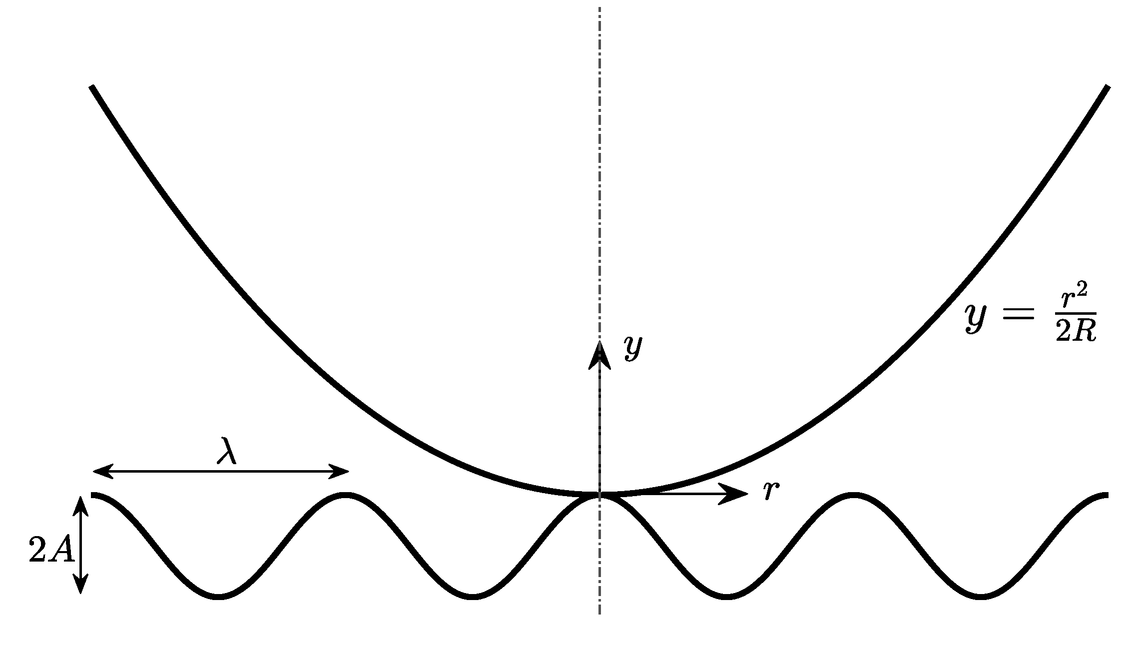
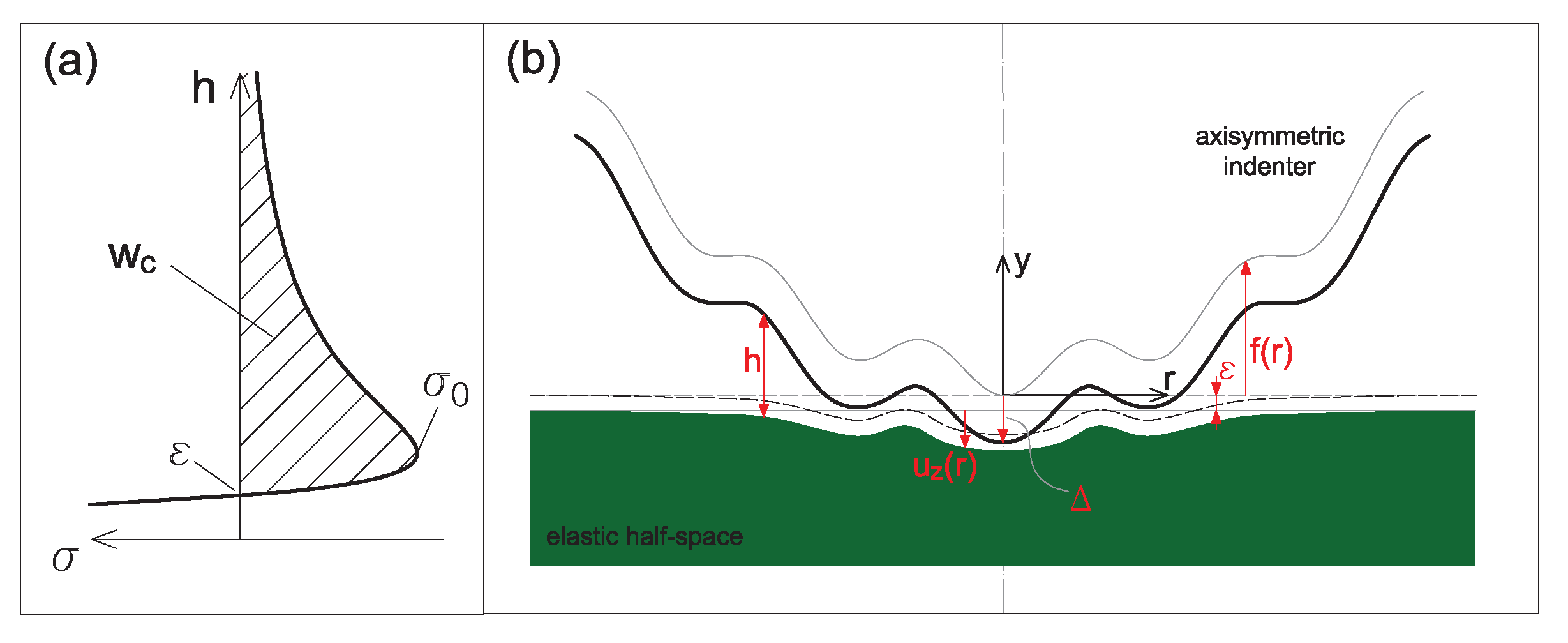
3. Numerical Solution

3.1. Axisymmetric BEM Formulation

In the previous section the JKR solution of the Guduru contact problem was briefly summarized. Several variants of the Guduru contact problem have been studied by different authors [20,21,22,24,28], nevertheless all of them assume full contact within the contact patch (a simply connected contact area). To overcome this limitation an axisymmetric Boundary Element Method (BEM) was developed assuming that the rigid sphere and the wavy halfspace interacts with a Lennard–Jones interaction law (LJ in the following, see Figure 2a)
σ h = 8 w c 3 ε ε h 3 ε h 9
where σ is the traction ( σ > 0 , when compressive), h is the gap and ε the equilibrium distance (the maximum tensile stress σ 0 = 16 w c 9 3 ε takes place at separation h = 3 1 / 6 ε ). BEM contact codes that use the LJ interaction law have been derived previously by several authors to solve contact problems similar to the one tackled here. For example Wu [31] solved the adhesive contact problem between a sphere and a longitudinal wavy surface, while Medina and Dini [32] studied the problem of an adhesive sphere squeezed against a rough substrate. Notice that other BEM solution strategies exist that are based on energy minimization [33,34].
The contact problem considered is equivalent to the case of a “rough” axisymmetric rigid Hertzian indenter squeezed against an elastic halfspace (Figure 2b). The Guduru gap function is written as
h = Δ + ε + r 2 2 R + A 1 cos 2 π r λ + u z r
where Δ > 0 when the Hertzian profile approaches the halfspace and u z r is the deflection of the elastic halfspace (see Figure 2b).
For axisymmetric frictionless contact problems [35,36]
u z r = 1 E * σ s G r , s s d s
where σ s is the pressure distribution, G r , s the Kernel function
G r , s = 4 π r K s r , s < r 4 π s K r s , s > r
and K k the complete elliptic integral of the first kind of modulus k.
After surveying the Literature on the topic [31,32,33,34,35,36,37], we developed an axisymmetric BEM inspired by the works of Greenwood [35] and Feng [36]. Assume the radial domain is discretized with N elements, so that we have M = N + 1 discretization points. To solve Equation (10) on a discrete domain, one needs to determine the elastic deflection u z r . A problem arises in evaluating the integral (11) as the kernel function G r , s is singular in s = r . The common approach is to discretize Equation (11) assuming that the pressure σ s has a simple form over a discrete element. To this end, the simplest approach is to assume that the pressure is constant over each element. Nevertheless, Greenwood [35] reported that this method may lead to suspicious results, particularly in the regions with strong pressure gradients and suggested using the method of the overlapping triangles [29], for which the pressure σ s has a triangular form. Hence the deflection at point r i due to a triangular pressure distribution being p j at r = r j and falling linearly to 0 at r = r j 1 and r = r j + 1 is
u z r i = u z , i = 1 E * G i j p j
where we have solved numerically the integral in Equation (11) to obtain G i j once for all. Notice that the kernel function singularity at r i = r j 1 and r i = r j + 1 is canceled by the pressure being 0 in r j 1 and r j + 1 , instead, for the singular point r i = r j , we considered a pressure equal to p j at r j 1 and r j + 1 rising linearly at 0 at r j superimposed to a constant pressure ring, equal to p j , in between the radii r j 1 and r j + 1 for which the displacement field is known analytically (see Appendix A). By defining the following quantities
H = h / ε 1 ; u = r Γ ; L = λ Γ ; P = p μ ε w c ; Γ = R 2 w c E * 1 / 3 ;
Equation (10) is written for the normalized gap H i (H vanishes for h = ε ) at each node i as:
H i = Δ + 1 2 μ u i 2 + A 1 cos 2 π u L + μ j = 1 N G i j P j
where μ = R w c 2 E * 2 ε 3 1 / 3 is the Tabor parameter, Δ = Δ / ε , A = A / ε , G i j = G i j / Γ and
P j = 8 3 μ 1 H j + 1 3 1 H j + 1 9
All the results that will be presented below were obtained using N = 500 discretization elements with a constant element size, which proved to be sufficient for obtaining converged solutions up to a Tabor parameter μ = 5 . Lower values of μ did not require such a mesh refinement, nevertheless, to avoid confusion, the same discretization was used along all the paper. Unless differently stated, in all the simulations the overall domain length was set equal to the sphere radius r max = R = 100 ε . The numerical code was implemented in MATLAB. Similarly to Feng [36] an efficient pseudo-archlength continuation scheme was implemented [38], which is needed to follow the system solution branches. Furthermore, to make the numerical solution of the nonlinear system of Equation (15) faster to solve, the system Jacobian was provided analytically to the numerical solver (“fsolve” in MATLAB) that implements a Newton–Raphson scheme.

3.2. Validation of the Numerical Results

First to assess the correctness of the numerical implementation, the BEM results are validated against those provided by Feng [36]. In Figure 3 the dimensionless normal load
W ¯ = W π w c R = 2 Γ 2 μ R ε 0 + P ( u ) u d u
is plotted as a function of the dimensionless approach Δ for μ = [ 1 , 2 , 3 ] . Markers refer to the data reported by Feng [36] (its Figure 3) while the solid black lines were obtained numerically using the BEM presented here. Red dots stand for the Bradley [23] rigid solution, which is compared to the numerical solution (solid black line) obtained with μ = 0.01 . All the curves are in perfect agreement.
Figure 4 shows the pull-off force W ¯ p u l l o f f (panel (a)) and the approach Δ p u l l o f f (panel (b)) at pull-off as a function of μ (the pull-off force W ¯ p u l l o f f is defined as the minimum of the W ( Δ ) curve). Blue stars have been obtained from Feng [36], while red squares have been obtained using the BEM developed here. The results we obtained for both load and approach at pull-off compare very favorably with those in [36].

4. Rigid Limit

The majority of the authors, who have tackled the Guduru contact problem, have focused their attention on the JKR limit, where it was clear since the early papers by Guduru [17] and Guduru and Bull [19] that substantial enhancement could be obtained, with few exceptions, as the works of Waters [22] and that of Ciavarella [24]. Waters et al. [22] developed a Maugis–Dugdale cohesive model for the Guduru problem that showed adhesion enhancement is mostly limited to the JKR regime. The cohesive model clearly depended on an additional parameter with respect to the JKR model, the Tabor parameter μ . Strictly speaking, Waters et al. [22] used the parameter introduced by Maugis [39], which anyway differs only by a small multiplicative factor from μ . Waters et al. [22] analysis showed that for small μ the pull-off detachment force converged to the Bradley rigid solution for the sphere, i.e., W ¯ B = 2 . Nevertheless, this holds only for a smooth sphere in contact with a flat halfspace. For example, let us assume λ R A , then the pull-off force in the rigid regime could be estimated by considering the contact between the first crest of the halfspace waviness and the sphere. The radius of curvature of the crest is
R 2 = λ 2 4 π 2 A R 4 π 2
and the composite radius
R * = 1 R + 4 π 2 R 1 R 4 π 2
hence the pull-off force of the sphere would be reduced by about factor 1 / 4 π 2 0.025 . Indeed, using the Rumpf–Rabinowicz model [25,26,27] Ciavarella [24] recognized this. Although analogous to the Guduru problem, the Rumpf–Rabinowicz model refers to a different geometry. It considers the contact between a large sphere of radius R and a rigid small hemisphere of radius r 2 placed on a rigid plane (see Figure 5).
Two competitive mechanisms for adhesion take place: while the radius of the hemisphere increases macroscopic adhesion increases due to the interaction with the hemisphere but decreases as the rigid plane gets further away from the countersurface, which, using r 2 = λ 2 4 π 2 A , can be written as [24]
W ¯ p u l l o f f = 1 1 + 4 π 2 α + 1 1 + R 4 π 2 α 2
where R = R / ε . Similar mechanisms are expected to be at play in the Guduru problem.
Assume that the rigid sphere and the wavy halfspace interact with a Lennard–Jones interaction law (9). From Equation (15), neglecting the elastic deformations, the dimensionless interfacial gap is
H θ = Δ + A θ 2 8 π 2 α + 1 cos θ
where θ = 2 π r λ has been introduced. Using Equations (16) and (17) the total load is
W ¯ r i g i d = 2 π π w c R 0 + σ ( H ) r d r = 4 A 3 π 2 α 0 + 1 H θ + 1 3 1 H θ + 1 9 θ d θ
which clarifies that at a given approach Δ the rigid solution depends only on two parameters α , A .
Notice that for a smooth sphere-flat contact one can use in the first integral of Equation (22) d H = r R d r and obtain that the rigid solution depends only on the adhesion energy and not on the shape of the potential. This cannot be done for the Guduru gap function, which implies that the Guduru rigid solution will be slightly affected by the shape of the interaction law used.
In Figure 6 the loading curves are shown for log 10 α = [ 4 , 2 , 1 , 0 , 1 ] and A = 1 . The solid black lines are the theoretical predictions based on Equation (22), while the red markers have been obtained numerically using the BEM with μ = 10 4 . Numerical and theoretical predictions are in perfect agreement, with the curve log 10 α = 4 corresponding to the Bradley [23] rigid solution for the smooth sphere (Equation (22))
W ¯ B Δ = 2 4 Δ 1 6 1 3 Δ 1 8
The curves dimensionless normal load W ¯ versus dimensionless approach Δ plotted in Figure 6 show that the pull-off force is not monotonically decreasing with α and that the critical approach at detachment is close to Δ 0 only for the smallest values of α . Figure 7 shows the pull-off force as a function of α for log 10 A = [ 3 , 0.5 , 0 , 1 , 2 , 4 ] (solid lines obtained as the minimum of (22), while red markers obtained numerically μ = 10 4 ). All the curves start at small α from the Bradley rigid solution W ¯ B , p u l l o f f = 2 (smooth sphere), while increasing α the pull-off force decays and, after a transition zone around α 1 , reaches a limit value at large α . It is shown that at large α and A the pull-off force can decrease by more than three orders of magnitude with respect to the smooth case. To allow a comparison the predictions of the Rumpf–Rabinowicz model are reported for log 10 R = [ 0 , 1 , 2 , 3 , 4 ] (blue dashed lines in Figure 7). First notice that, while the rigid limit of the Guduru problem depends on α , A , the Rumpf–Rabinowicz model depends on α , R . Both the models show a similar decay with α , but they give two different limits for large α . In the Rumpf–Rabinowicz model, a large α implies a very small hemisphere ( R / r 2 = 4 π 2 α ), hence the case of a large sphere interacting with a smooth plane is retrieved. In the rigid Guduru model, A and λ = λ / ε are not coupled, hence increasing α leads to a vanishing wavelength of the sinusoid but does not affect A , which gives the observed adhesion reduction.

5. Numerical Results

5.1. Effect of the Tabor Parameter

In the previous subsections we have discussed two limits of the Guduru contact problem: the JKR and the rigid limit. Here the transition from one limit to the other is investigated numerically by using the BEM introduced in Section 3.1. Figure 8 shows the pull-off force as a function of the Tabor parameter μ for λ = 20 , and A = 0.1 , 1 , 10 . Small waviness amplitude A = 0.1 (red circles) slightly perturbs the solution of the smooth sphere. Indeed at low Tabor parameter the pull-off force is equal to W ¯ p u l l o f f 1.75 , while at higher μ it gets slightly larger than 1.5 . In all the range between μ = 0.01 and μ = 5 the pull-off force remains in between the rigid and JKR values (2 and 1.5 respectively). Increasing the waviness amplitude by a factor 10 ( A = 1 , green squares) completely changes the picture. Figure 8 shows that there exist three distinct regimes: (i) the rigid, (ii) the transition and (iii) the JKR regime. The pull-off force remains very small and equal to the rigid limit (dot-dashed line) up to μ 0.25 , then starts to increase up to about W ¯ p u l l o f f 3.2 for μ 1 and for μ > 1 tends to the JKR limit (Equation (5), dashed line). By further increasing the waviness amplitude leads to smaller pull-off forces not only in the rigid limit, but also at large Tabor parameters μ . We have indicated in Figure 8 that at μ 5 the JKR prediction of the pull-off force is W ¯ p u l l o f f 20 , while numerical results give W ¯ p u l l o f f 1.1 .
Figure 9 shows respectively the dimensionless gap H (a) and the corresponding tractions P (b) for λ = 20 , A = 1 and μ = 0.15 , 0.67 , 5 (respectively solid, dotted, dot-dashed line) and A = 10 , μ = 5 (dashed line) at the pull-off point. Focusing on the three curves corresponding at A = 1 one recognizes that at low Tabor parameter μ = 0.15 the maximum tensile force is reached when the sphere first touches the waviness crest, while for high Tabor parameter ( μ = 5 , pink dot-dashed line) the typical pressure spike appears at the boundary of the contact patch. In the intermediate regime μ = 0.67 the maximum pull-off force is reached when the second crest first touches the sphere. Nevertheless, the material is too rigid to deform and the gap remains large at the first throat providing small adhesive tractions. It is useful to compare the solutions obtained for μ , A = 5 , 1 with those for μ , A = 5 , 10 . In the latter case Figure 8 showed that JKR theory highly overestimates the pull-off force obtained numerically. Indeed, Figure 9 shows that the contact patch is clustered on the waviness peaks and axisymmetric grooves (internal cracks) appear, which destroy the well known enhancement mechanism of the Guduru geometry.
To better study the effect of the waviness amplitude A , Figure 10 shows the dimensionless pull-off force in absolute value as a function of the ratio A / λ for λ = 5 , 20 , 30 , 50 , R = [ 50 , 100 , 200 ] and for a fixed μ = 3 (see legend therein). For each value of λ Equation (5) was used to determine the pull-off force predicted by the JKR model (dashed black lines), while numerical results obtained with BEM are reported with markers (see legend in Figure 10). For amplitude to wavelength ratio below A / λ 10 1 the numerical simulations and the theoretical results are in very good agreement. For very small waviness amplitude the JKR result for the smooth sphere is obtained W ¯ p u l l o f f = 1.5 , while increasing A / λ adhesion enhancement takes place up to W ¯ p u l l o f f 10 for λ = 50 . It appears that longer wavelengths foster adhesion enhancement. For A / λ 10 1 , the pull-off force suddenly decreases and, for larger W ¯ p u l l o f f , decays approximately with a power law, without showing a clear threshold for “stickiness” (complete elimination of adhesion), contrary to other recent theories on random roughness [40,41]. It is shown that the sphere radius markedly influences the pull-off decay, but, in the parametric region explored, it slightly affects the threshold A / λ 10 1 at which the abrupt transition from adhesion enhancement to reduction takes place.
In Figure 11 we have replotted the data in Figure 10 as effective adhesion energy w ¯ c , e f f = w c , e f f / w c versus the Johnson parameter α K L J . Indeed, based on Kesari and Lew [21] envelope solution, Ciavarella [24] showed that in the JKR regime the effective adhesive energy at pull-off depends only on the Johnson parameter α K L J , i.e.,
w ¯ c , e f f = 2 3 W ¯ p u l l o f f = 1 + 1 π α K L J 2
which is shown as a solid blue line in Figure 11. On the contrary, a competitive mechanism has been proposed by Persson and Tosatti [13], which tends to reduce the effective adhesive energy due to surface roughness in randomly rough surfaces. Persson and Tosatti [13] criterion reads
w c , e f f = w c A t r u e A a p p U e l A a p p
where A a p p is the apparent contact area, A t r u e is the real contact area, increased due to the substrate roughness, and U e l is the elastic strain energy stored at full contact. The real contact area A t r u e can be written as [13]
A t r u e = 2 π A a p p d r r 1 + 1 2 h 2
= 2 π 0 a a p p d r r 1 + 1 2 2 π A λ 2 sin 2 2 π r λ
where a a p p is the apparent contact radius. Dividing Equation (27) by A a p p = π a a p p 2 , it can be derived that for large enough a a p p / λ
A t r u e A a p p 1 + π A λ 2 .
In Figure 10 we obtained the largest enhancement of the pull-off force (up to a factor 10) at about A / λ 10 1 , where Equation (28) would give A t r u e / A a p p 1.03 (notice that w ¯ c , e f f = 2 3 W ¯ p u l l o f f ), hence, in the following, we will neglect this contribution.
For a single scale waviness
U e l A a p p = E 4 1 ν 2 d 2 q q C q = π E 4 1 ν 2 A 2 λ
hence
w ¯ c , e f f = 1 1 2 π 1 α K L J 2
which is reported as a dot-dashed red line in Figure 11. The numerical results we obtained, plotted with markers in Figure 11, show that at large α K L J the numerical results we obtained closely follow Equation (24). For smaller α K L J , instead, w ¯ c , e f f drops suddenly and decays by further reducing α K L J with a strong dependence on the waviness wavelength and sphere radius. Instead, the Persson–Tosatti energetic argument for adhesion reduction seems to give a lower bound to the effective work of adhesion.

5.2. Hysteresis Cycle

It is well known that in adhesive contact mechanics different loading paths can be followed in loading and unloading a contact pair, which leads also to hysteretical energy dissipation. Here we show how this gets affected by the waviness amplitude A by proposing two representative examples. In Figure 12 the loading curve obtained via BEM numerical simulation is plotted as a solid red line for μ = 4 , A = 0.4 , R = 100 and λ = 10 . On the same graph, the JKR loading curve for the smooth sphere (black dot-dashed curve) and for the Guduru geometry (blue dashed curve, Equation (5)) are plotted. Figure 12 shows that the numerical and the theoretical curves are very close each other and the maximum adhesive force reached is about W ¯ p u l l o f f 2 giving a certain enhancement with respect to the smooth case. A possible loading path (in displacement control) is shown by the arrows. The jump-in and -out instability are labeled with numbers from “1” to “6” for the loading stage and with letters from “a” to “f” during unloading. Looking at Figure 12 one sees the hysteretical dissipation (proportional to the area enclosed in the hysteretical loop in Figure 12), which could be well estimated by adopting the JKR model (Equation (5)).
Nevertheless, the amount of dissipation is strongly influenced by the ratio A / λ and the results obtained by the JKR model (Equation (5)) may be strongly misleading. In Figure 13 the curve dimensionless normal load W ¯ versus Δ / μ obtained numerically (red solid line) is plotted for the same parameters of Figure 12 but for A = 3 . Together with the BEM numerical results the JKR curve for the smooth sphere (black dot-dashed line) and for the Guduru geometry (blue dashed line) are shown. One immediately recognizes that the JKR model (blue dashed line) is very far from the actual loading curve (solid red curve). While the sphere approaches the wavy halfspace the JKR model predicts very large fluctuations of the normal load and relative jumps from one branch to the other that would lead to very high energy dissipation. The BEM solution, instead, gives much smaller undulations of the loading curve and smaller jumps-in and -out contact.

5.3. Adhesion Map

To clarify the effect of A, λ and μ on the pull-off force W ¯ p u l l o f f we fixed the sphere radius R = 100 and change μ = 10 1 , 5 and A / λ = [ 10 3 , 10 0 ] . Figure 14 and Figure 15 shows the contour plot of the pull-off force respectively for λ = 20 and λ = 5 . One immediately notices that larger adhesive forces are reached with longer wavelengths. Figure 14 shows that adhesion enhancement happens in a limited parameter region. For very low ratio A / λ the contact problem reduces to that of the smooth sphere on a smooth halfspace, hence by changing the Tabor parameter from μ = 0.01 to μ = 5 one moves from the Bradley W ¯ p u l l o f f = 2 to the JKR solution W ¯ p u l l o f f = 1.5 . Increasing A / λ for small Tabor parameter ( μ < 10 0.6 0.25 ) leads to a strong reduction of the pull-off force, as indeed we are in the range where the rigid solution of the Guduru problem holds (cfr. Section 2, Figure 7). Notice that keeping λ constant and increasing A / λ leads to both increasing of A and α in Figure 7 heading to very strong reduction of the macroscopic pull-off force. Instead, if A / λ is increased at large Tabor parameter ( μ 0.25 for λ = 20 ), adhesion enhancement takes place and high pull-off forces can be reached (in Figure 14 up to W ¯ p u l l o f f 4 for μ 5 ). Contrary to JKR theory predictions, further increasing of the amplitude to wavelength ratio A / λ does not lead to stronger adhesive forces, but adhesion is destroyed by roughness.

6. Conclusions

In this paper we have reconsidered the Guduru adhesive contact problem. The rigid solution has been derived, which has been shown to depend only on two parameters: the dimensionless waviness amplitude A and the dimensionless parameter α = A R / λ 2 . It has been shown that increasing A and α reduces the macroscopic pull-off force by orders of magnitude due to the effect of roughness. Secondly, by using a BEM numerical code with Lennard–Jones interaction law, we have investigated the effects of the waviness wavelength, amplitude and of the sphere Tabor parameter on the adhesion enhancement. It has been shown that adhesion enhancement is limited to a certain region of the plane A / λ versus μ . In particular, at low Tabor parameter increasing the ratio A / λ tends to destroy adhesion. For large Tabor parameters increasing the ratio A / λ first increases adhesion due to the Guduru enhancement mechanism, but later, for A / λ greater than about 10 1 , the waviness amplitude gets too large, internal cracks appear and macroscopic adhesion reduces strongly. We have shown that in this region using the JKR model to estimate both the pull-off force and the dissipated energy by hysteresis leads to very large errors as the hypothesis of compact contact area does not hold.
The enhancement effect is well captured by the Johnson parameter as derived by Ciavarella–Kesari–Lew [21,24], and is much larger than the Persson–Tosatti enhancement [13] in terms of increase of real contact area due to roughness. The Persson–Tosatti energetic argument for adhesion reduction seems to give a lower bound to the effective work of adhesion.
The axisymmetric waviness in the Guduru contact problem is highly idealized with respect to more common randomly fractal roughness, hence it is difficult to give reasonable estimates of the parameters we have introduced in our model for a fractal randomly rough surface. The analysis made is intended to shed light into the problem of adhesion enhancement with a potential application to the development of nano- and micro-mechanical systems and of bioinspired adhesives. Experimental measurements have been reported by Santos et al. [42], which show how echinoderms’ tube feet exploit adhesion enhancement to increase the interfacial toughness on rough substrates. Santos et al. [42] tried to explain the interfacial toughening accounting for an increased contact area obtained when the echinoderm feet conforms to the rough substrate. We have found that adhesion enhancement may be obtained also when the latter effect is negligible.
When rough surfaces are idealized by spherical caps, a very small radius of curvature is expected at the finest scale, which suggests asperity contact takes place at very low Tabor parameters, hence adhesion enhancement seems to be very unlikely. At present, the only viable route to adhesion enhancement seems to be the design of an ad-hoc macroscopic roughness profile.

Author Contributions

Conceptualization, A.P. and M.C.; Methodology, Validation, Investigation, Writing—original draft preparation, A.P.; writing—review and editing, A.P. and M.C.; Supervision: M.C.; All authors have read and agreed to the published version of the manuscript.

Funding

This research received no external funding.

Acknowledgments

A.P. and M.C. acknowledge the support by the Italian Ministry of Education, University and Research under the Programme Department of Excellence Legge 232/2016 (Grant No. CUP-D94I18000260001). A.P. is thankful to the DFG (German Research Foundation) for funding the project PA 3303/1-1. A.P. acknowledges support from “PON Ricerca e Innovazione 2014-2020-Azione I.2” - D.D. n. 407, 27/02/2018, bando AIM (Grant No. AIM1895471).

Conflicts of Interest

The authors declare no conflict of interest.

Appendix A. BEM Formulation with Constant Pressure Discrete Elements

Equation (10) constitutes the nonlinear problem to be solved. A problem arises in evaluating the integral (11) as the kernel function G r , s is singular in s = r . The common approach is to discretize Equation (11) assuming that the pressure σ s has a simple form over a discrete element. To this end the simplest approach is to assume that the pressure is constant over each element. For a constant pressure p ¯ acting over the ring c 1 < r < c 2 the deflection at r of a single half-space is
u z r = 4 p ¯ π E * F c 2 , r F c 1 , r
where from Johnson [29]
F c , r = c E r c , r c r E c r 1 c r 2 K c r , r > c
being K k and E k respectively the complete elliptic integrals of first and second kind with modulus k.
Assume we have discretized the surface in N elements, so that we have M = N + 1 discretization points. The deflection at point r i due to a constant pressure p ¯ j ring in between the radii r j and r j + 1 is
u z r i = 4 p ¯ j π E * F r j + 1 , r i F r j , r i = 1 E * G i j p ¯ j
G i j = 4 π F r j + 1 , r i F r j , r i
where the term G i j within square brackets depends only on the nodal coordinates, hence by varying i , j = 1 , . . . , M all the terms can be computed once for all.

References

  1. Ciavarella, M.; Joe, J.; Papangelo, A.; Barber, J.R. The role of adhesion in contact mechanics. J. R. Soc. Interface 2019, 16, 20180738. [Google Scholar] [CrossRef] [PubMed] [Green Version]
  2. Tadmor, R.; Das, R.; Gulec, S.; Liu, J.; N’guessan, H.; Shah, M.; Wasnik, P.; Yadav, S.B. Solid–liquid work of adhesion. Langmuir 2017, 33, 3594–3600. [Google Scholar] [CrossRef] [PubMed]
  3. Vakis, A.I.; Yastrebov, V.A.; Scheibert, J.; Nicola, L.; Dini, D.; Minfray, C.; Molinari, J.F. Modeling and simulation in tribology across scales: An overview. Tribol. Int. 2018, 125, 169–199. [Google Scholar] [CrossRef]
  4. Gorb, S.; Varenberg, M.; Peressadko, A.; Tuma, J. Biomimetic mushroom-shaped fibrillar adhesive microstructure. J. R. Soc. Interface 2007, 4, 271–275. [Google Scholar] [CrossRef] [PubMed] [Green Version]
  5. Skelton, S.; Bostwick, M.; O’Connor, K.; Konst, S.; Casey, S.; Lee, B.P. Biomimetic adhesive containing nanocomposite hydrogel with enhanced materials properties. Soft Matter 2013, 9, 3825–3833. [Google Scholar] [CrossRef]
  6. Tang, J.; Li, J.; Vlassak, J.J.; Suo, Z. Adhesion between highly stretchable materials. Soft Matter 2016, 12, 1093–1099. [Google Scholar] [CrossRef]
  7. Murphy, M.P.; Aksak, B.; Sitti, M. Gecko-inspired directional and controllable adhesion. Small 2009, 5, 170–175. [Google Scholar] [CrossRef]
  8. Papangelo, A.; Lovino, R.; Ciavarella, M. Electroadhesive sphere-flat contact problem: A comparison between DMT and full iterative finite element solutions. Tribol. Int. 2020. [Google Scholar] [CrossRef]
  9. Sahli, R.; Pallares, G.; Papangelo, A.; Ciavarella, M.; Ducottet, C.; Ponthus, N.; Scheibert, J. Shear-induced anisotropy in rough elastomer contact. Phys. Rev. Lett. 2019, 122, 214301. [Google Scholar] [CrossRef] [Green Version]
  10. Papangelo, A.; Scheibert, J.; Sahli, R.; Pallares, G.; Ciavarella, M. Shear-induced contact area anisotropy explained by a fracture mechanics model. Phys. Rev. E 2019, 99, 053005. [Google Scholar] [CrossRef] [Green Version]
  11. Papangelo, A.; Ciavarella, M. On mixed-mode fracture mechanics models for contact area reduction under shear load in soft materials. J. Mech. Phys. Solids 2019, 124, 159–171. [Google Scholar] [CrossRef] [Green Version]
  12. Ciavarella, M.; Papangelo, A. On the Degree of Irreversibility of Friction in Sheared Soft Adhesive Contacts. Tribol. Lett. 2020, 68, 81. [Google Scholar] [CrossRef]
  13. Persson, B.N.J.; Tosatti, E. The effect of surface roughness on the adhesion of elastic solids. J. Chem. Phys. 2001, 115, 5597–5610. [Google Scholar] [CrossRef] [Green Version]
  14. Violano, G.; Afferrante, L.; Papangelo, A.; Ciavarella, M. On stickiness of multiscale randomly rough surfaces. J. Adhes. 2019, 1–19. [Google Scholar] [CrossRef] [Green Version]
  15. Fuller, K.N.G.; Tabor, D. The effect of surface roughness on the adhesion of elastic solids. Proc. R. Soc. Lond. A Math. Phys. Sci. 1975, 345, 327–342. [Google Scholar]
  16. Briggs, G.A.D.; Briscoe, B.J. The effect of surface topography on the adhesion of elastic solids. J. Phys. D Appl. Phys. 1977, 10, 2453. [Google Scholar] [CrossRef]
  17. Guduru, P.R. Detachment of a rigid solid from an elastic wavy surface: Theory. J. Mech. Phys. Solids 2007, 55, 445–472. [Google Scholar] [CrossRef]
  18. Johnson, K.L.; Kendall, K.; Roberts, A. Surface energy and the contact of elastic solids. Proc. R. Soc. Lond. A Math. Phys. Sci. 1971, 324, 301–313. [Google Scholar]
  19. Guduru, P.R.; Bull, C. Detachment of a rigid solid from an elastic wavy surface: Experiments. J. Mech. Phys. Solids 2007, 55, 473–488. [Google Scholar] [CrossRef]
  20. Kesari, H.; Doll, J.C.; Pruitt, B.L.; Cai, W.; Lew, A.J. Role of surface roughness in hysteresis during adhesive elastic contact. Philos. Philos. Mag. Lett. 2010, 90, 891–902. [Google Scholar] [CrossRef] [Green Version]
  21. Kesari, H.; Lew, A.J. Effective macroscopic adhesive contact behavior induced by small surface roughness. J. Mech. Phys. Solids 2011, 59, 2488–2510. [Google Scholar] [CrossRef]
  22. Waters, J.F.; Lee, S.; Guduru, P.R. Mechanics of axisymmetric wavy surface adhesion: JKR–DMT transition solution. Int. J. Solids Struct. 2009, 46, 1033–1042. [Google Scholar] [CrossRef] [Green Version]
  23. Bradley, R.S. The cohesive force between solid surfaces and the surface energy of solids. Lond. Edinb. Dublin Philos. J. Sci. 1932, 13, 853–862. [Google Scholar] [CrossRef]
  24. Ciavarella, M. On roughness-induced adhesion enhancement. J. Strain Anal. Eng. Des. 2016, 51, 473–481. [Google Scholar] [CrossRef] [Green Version]
  25. Rumpf, H. Particle Technology; Chapman & Hall: London, UK, 1990. [Google Scholar]
  26. Rabinovich, Y.I.; Adler, J.J.; Ata, A.; Singh, R.K.; Moudgil, B.M. Adhesion between nanoscale rough surfaces: I. Role of asperity geometry. J. Colloid Interface Sci. 2000, 232, 10–16. [Google Scholar] [CrossRef]
  27. Rabinovich, Y.I.; Adler, J.J.; Ata, A.; Singh, R.K.; Moudgil, B.M. Adhesion between nanoscale rough surfaces: II. Measurement and comparison with theory. J. Colloid Interface Sci. 2000, 232, 17–24. [Google Scholar] [CrossRef]
  28. Ciavarella, M. An upper bound to multiscale roughness-induced adhesion enhancement. Tribol. Int. 2016, 102, 99–102. [Google Scholar] [CrossRef] [Green Version]
  29. Johnson, K.L. Contact Mechanics; Cambridge University Press: Cambridge, UK, 1985. [Google Scholar]
  30. Johnson, K.L. The adhesion of two elastic bodies with slightly wavy surfaces. Int. J. Solids Struct. 1995, 32, 423–430. [Google Scholar] [CrossRef]
  31. Wu, J.J. Numerical Analyses on the Adhesive Contact between a Sphere and a Longitudinal Wavy Surface. J. Adhes. 2014, 91, 381–408. [Google Scholar] [CrossRef]
  32. Medina, S.; Dini, D. A numerical model for the deterministic analysis of adhesive rough contacts down to the nano-scale. Int. J. Solids Struct. 2014, 51, 2620–2632. [Google Scholar] [CrossRef] [Green Version]
  33. Rey, V.; Anciaux, G.; Molinari, J.F. Normal adhesive contact on rough surfaces: Efficient algorithm for FFT-based BEM resolution. Comput. Mech. 2017, 60, 69–81. [Google Scholar] [CrossRef] [Green Version]
  34. Li, Q.; Pohrt, R.; Popov, V.L. Adhesive Strength of Contacts of Rough Spheres. Front. Mech. Eng. 2019, 5, 7. [Google Scholar] [CrossRef] [Green Version]
  35. Greenwood, J.A. Adhesion of elastic spheres. Proc. R. Soc. Lond. Ser. A Math. Phys. Eng. Sci. 1997, 453, 1277–1297. [Google Scholar] [CrossRef]
  36. Feng, J.Q. Contact behavior of spherical elastic particles: A computational study of particle adhesion and deformations. Colloids Surfaces Physicochem. Eng. Asp. 2000, 172, 175–198. [Google Scholar] [CrossRef]
  37. Attard, P.; Parker, J.L. Deformation and adhesion of elastic bodies in contact. Phys. Rev. A 1992, 46, 7959. [Google Scholar] [CrossRef]
  38. Nayfeh, A.H.; Balachandran, B. Applied Nonlinear Dynamics: Analytical, Computational, and Experimental Methods; John Wiley & Sons: Hoboken, NJ, USA, 2008. [Google Scholar]
  39. Maugis, D. Adhesion of spheres: The JKR-DMT transition using a Dugdale model. J. Colloid Interface Sci. 1992, 150, 243–269. [Google Scholar] [CrossRef]
  40. Pastewka, L.; Robbins, M.O. Contact between rough surfaces and a criterion for macroscopic adhesion. Proc. Natl. Acad. Sci. USA 2014, 111, 3298–3303. [Google Scholar] [CrossRef] [Green Version]
  41. Ciavarella, M. Universal features in “stickiness” criteria for soft adhesion with rough surfaces. Tribol. Int. 2020, 146, 106031. [Google Scholar] [CrossRef] [Green Version]
  42. Santos, R.; Gorb, S.; Jamar, V.; Flammang, P. Adhesion of echinoderm tube feet to rough surfaces. J. Exp. Biol. 2005, 208, 2555–2567. [Google Scholar] [CrossRef] [Green Version]
Figure 1. The geometry of the axisymmetric contact problem. A rigid sphere of radius R indents an elastic halfspace with an axisymmetric waviness of wavelength λ and amplitude A. The sphere is approximated by a Hertzian profile.
Lubricants 08 00090 g001
Figure 2. (a) Lennard–Jones interaction law. (b) Equivalent representation of the considered contact problem in the undeformed configuration (grey lines) and after applying a certain remote displacement Δ (black lines).
Lubricants 08 00090 g002
Figure 3. Dimensionless normal load W ¯ as a function of the approach Δ for μ = [ 1 , 2 , 3 ] as reported by Feng [36] (markers) and as obtained here numerically (solid black line). Red dots show the Bradley [23] rigid solution, which is compared to the numerical solution (solid black line) obtained with μ = 0.01 .
Lubricants 08 00090 g003
Figure 4. (a) Pull-off force W ¯ p u l l o f f and (b) approach Δ p u l l o f f at pull-off as a function of the Tabor parameter μ = [ 10 2 , 5 ] . Red squares were obtained with the presented Boundary Element Method (BEM) scheme, while blue asterisks were obtained from Feng [36].
Lubricants 08 00090 g004
Figure 5. Left panel: simplified sketch of the Rumpf–Rabinowicz model. Right panel: simplified sketch of the Guduru model.
Lubricants 08 00090 g005
Figure 6. Loading curves for the rigid model. Solid lines have been obtained from Equation (22), while red markers are numerical solutions for μ = 10 4 . The curves are obtained for log 10 α = [ 4 , 2 , 1 , 0 , 1 ] and A = 1 .
Lubricants 08 00090 g006
Figure 7. Pull-off force as a function of the parameter α (log scale) obtained using the rigid solution of the Guduru model (Equation (22), solid black line) and the Rumpf–Rabinowicz model (Equation (20), blue dashed line), while red squares are numerical solutions for μ = 10 4 . For the Guduru rigid model the curves are obtained for log 10 A = [ 3 , 0.5 , 0 , 1 , 2 , 4 ] , while for the Rumpf–Rabinowicz model log 10 ( R ) = [ 0 , 1 , 2 , 3 , 4 ] .
Lubricants 08 00090 g007
Figure 8. Pull-off force W ¯ p u l l o f f (absolute value) as a function of the Tabor parameter μ for λ = 20 , R = 100 and A = 0.1 , 1 , 10 , respectively red circles, green squares and blue triangles. Dot-dashed lines mark the rigid limit (22) whil dashed lines the Johnson–Kendall–Roberts (JKR) limit (5). For A = 10 at μ = 5 the JKR limit would give W ¯ p u l l o f f 20 .
Lubricants 08 00090 g008
Figure 9. (a) Dimensionless gap H and (b) dimensionless tractions P versus the radial coordinate r / ε at the pull-off point for λ = 20 , R = 100 and varying μ and A (for both panels please refer to the legend placed in panel (b)).
Lubricants 08 00090 g009
Figure 10. Dimensionless pull-off force in absolute value as a function of the ratio A / λ for the four cases λ = 5 , 20 , 30 , 50 , R = [ 50 , 100 , 200 ] and for a fixed μ = 3 (see legend). Dashed lines stand for the pull-off force predicted by the JKR model (Equation (5)), markers for BEM numerical results, while the dot-dashed line is a guide to the eye.
Lubricants 08 00090 g010
Figure 11. The data showed in Figure 10 are reported here as effective adhesion energy w ¯ c , e f f = w c , e f f / Δ γ versus the α K L J for the four cases λ = 5 , 20 , 30 , 50 , R = [ 50 , 100 , 200 ] and for a fixed μ = 3 (see legend). The dot-dashed line stands for the reduction criterion of Persson and Tosatti [13], the solid line for the enhancement criterion of Ciavarella [24] based on the Kesari and Lew [21] solution of the Guduru problem and the dashed line is a guide to the eye.
Lubricants 08 00090 g011
Figure 12. The dimensionless normal load W ¯ is plotted versus Δ / μ . The curve is obtained via BEM numerical simulation (solid red line) for μ = 4 , A = 0.4 , R = 100 and λ = 10 . The JKR curve for a smooth sphere (dot-dashed black line) and for the Guduru geometry (blue dashed line, Equation (5)) are also shown. Loading and unloading paths are indicated by arrows and the jump-in and -out contact points are respectively labeled by numbers from “1” to “6” and letters from “a” to “f”.
Lubricants 08 00090 g012
Figure 13. The dimensionless normal load W ¯ is plotted versus Δ / μ . The curve is obtained via BEM numerical simulation (solid red line) for μ = 4 , A = 3 , R = 100 and λ = 10 . The JKR curve for a smooth sphere (dot-dashed black line) and for the Guduru geometry (Equation (5)) are also shown. Loading and unloading paths are indicated by arrows and the jump-in and -out contact points are respectively labeled by numbers from “1” to “6” and letters from “a” to “f”.
Lubricants 08 00090 g013
Figure 14. Contour plot of the dimensionless pull-off force (absolute value) as a function of μ = 10 1 , 5 and A / λ = [ 10 3 , 10 0 ] for λ = 20 .
Lubricants 08 00090 g014
Figure 15. Contour plot of the dimensionless pull-off force (absolute value) as a function of μ = 10 1 , 5 and A / λ = [ 10 2 , 10 0 ] for λ = 5 .
Lubricants 08 00090 g015

