Optimizing Machine Learning Algorithms for Improving Prediction of Bridge Deck Deterioration: A Case Study of Ohio Bridges

Abstract

The deterioration of a bridge’s deck endangers its safety and serviceability. Ohio has approximately 45,000 bridges that need to be monitored to ensure their structural integrity. Adequate prediction of the deterioration of bridges at an early stage is critical to preventing failures. The objective of this research was to develop an accurate model for predicting bridge deck conditions in Ohio. A comprehensive literature review has revealed that past researchers have utilized different algorithms and features when developing models for predicting bridge deck deterioration. Since, there is no guarantee that the use of features and algorithms utilized by past researchers would lead to accurate results for Ohio’s bridges, this research proposes a framework for optimizing the use of machine learning (ML) algorithms to more accurately predict bridge deck deterioration. The framework aims to first determine “optimal” features that can be related to deck deterioration conditions, specifically in the case of Ohio’s bridges by using various feature-selection methods. Two feature-selection models used were XGboost and random forest, which have been confirmed by the Boruta algorithm, in order to determine the features most relevant to deck conditions. Different ML algorithms were then used, based on the “optimal” features, to select the most accurate algorithm. Seven machine learning algorithms, including single models such as decision tree (DT), artificial neural networks (ANNs), k-nearest neighbors (k-NNs), logistic regression (LR), and support vector machines (SVRs), as well as ensemble models such as Random Forest (RF) and eXtreme gradient boosting (XGboost), have been implemented to classify deck conditions. To validate the framework, results from the ML algorithms that used the “optimal” features as input were compared to results from the same ML algorithms that used the “most common” features that have been used in previous studies. On a dataset obtained from the Ohio Department of Transportation (ODOT), the results indicated that the ensemble ML algorithms were able to predict deck conditions significantly more accurately than single models when the “optimal” features were utilized. Although the framework was implemented using data obtained from ODOT, it can be successfully utilized by other transportation agencies to more accurately predict the deterioration of bridge components.

1. Introduction

The deterioration of infrastructure such as bridges has always been a concern for transportation agencies [1]. The maintenance, repair, and replacement (MRR) of bridges contribute to increased expenditure. Bridges are one of the essential components of our roadways [2]. The function of connecting different geographic areas makes bridges critical infrastructure. Frequent use of bridges accelerates their deterioration and complicates the implementation of bridge-management systems (BMSs). BMSs are implemented by transportation agencies to analyze bridge conditions, predict bridge deterioration, find the most efficient strategies of maintenance, and then prioritize and optimize them.

There are approximately 45,000 bridges in the state of Ohio [3], and every year, a significant amount of money is spent to repair and maintain them. The deterioration of bridges’ components significantly affects their integrity and structural safety [4]. It is crucial to model and predict the future deterioration of bridges under different environmental and location-specific conditions, among others, to forecast when a specific structure could be expected to begin to degrade or display signs of failure [2]. Furthermore, the ability to accurately predict the conditions of bridges may help ensure the proper and effective distribution of funds allocated for the maintenance, rehabilitation, and repair of bridges. This ability can also be helpful when determining which type of structure should be considered for a specific location [5].

Previous studies focused on modelling and analyzing bridge deterioration using a historical bridge inspection database [2]. Each state DOT maintains such a database. For example, the Ohio Department of Transportation (ODOT) maintains a comprehensive database of all bridges in Ohio, called AssetWise [3]. AssetWise is a web-based application that includes inventory and appraisal (inspection) data that stretches back several decades. A typical interval inspection is between 24 to 48 months, but an owner may request more frequent inspections [2]. Bridge inventories contain more than 130 different features of the bridges such as age, district, deck area, number of spans, etc. Moreover, they list the condition of various elements of the bridge such as substructure, superstructure, and deck, which make the analyses easier for researchers. Because bridge decks are more vulnerable to damage and because the serviceability of bridges depends heavily upon them [3,6,7], this study will focus on determining the rate of deterioration of bridge decks.

Predicting the condition of bridges has always been a challenging issue among scholars and transportation agencies, given the various options available such as statistical and machine learning techniques [8]. Nowadays, with the growing field of artificial intelligence (AI), scholars and transportation agencies are more interested in using these techniques, which typically yield more accurate predictions compared to statistical methods [9,10]. However, there are various ML models to implement, from simple algorithms such as kNN and SVM to more complex methods such as xGBoost and random forest, which are referred to as ensemble models. Therefore, choosing the most accurate ML model is an important issue that needs to be addressed.

Furthermore, a comprehensive literature review has revealed that past researchers have utilized different features when developing models for predicting bridge deck deterioration. Some of these features were common among researchers such as age, location of the bridge, and average daily traffic, while other features were unique. Since the accuracy of the prediction models depends on the set of features utilized, the characteristics of the data, and the chosen algorithm, there is a need for developing a framework for optimizing the use of ML algorithms to more accurately predict bridge deck deterioration [2]. The needed framework should provide a mechanism for (1) selecting the best set of features that are most related to bridge deterioration to use as input to the ML algorithms, and (2) selecting the most adequate ML algorithm.

The research described in this paper proposes such a framework to more accurately predict bridge deck deterioration using proper feature selection methods. The research methodology consisted of the following: (a) A comprehensive literature review which included three main parts was conducted. First, the statistical techniques used by past researchers for predicting bridge condition were reviewed. Secondly, ML techniques used by past researchers for predicting bridge deterioration were reviewed. Finally, previous studies on feature-selection methods were reviewed. (b) The NBI database was analyzed to see if it contained all the needed information. (c) The most popular ML algorithms were implemented to determine the most related features and the highest prediction accuracy. (d) The most accurate algorithm was identified and the hyperparameters for each model were optimized for evaluating each model’s accuracy, then feature selection models proposed in this research were compared to models that used the most common features. Each task is described in more detail in the following sections.

2. Research Background

According to studies, there are two methods for predicting bridge deterioration [5]. The first method utilizes statistical techniques such as Markov chains to statistically evaluate the effects of bridge characteristics on variations in bridge conditions and predict future bridge conditions. The second method utilizes ML algorithms.

Table 1. Reviewed studies that developed bridge deterioration prediction techniques.

Author	Year	AI	Statistic
Manafpour et al. [5]	2018		X
Chang et al. [6]	2018		X
Srikanth and Arockiasamy [11]	2019	X
Alsharqawi et al. [12]	2019	X
Nguyen and Dinh [13]	2019	X
Lu et al. [14]	2019	X
Lim et al. [15]	2019	X
Ilbeigi et al. [2]	2020		X
Martinez et al. [1]	2020	X
Abedin et al. [16]	2021	X

lists previous research conducted using both methods.

2.1. Statistical Techniques to Predict Bridge Deterioration

Ilbeigi et al. used an ordinal regression model to predict future bridge conditions; they focused on historical data in Ohio from 1992 to 2017 pertaining to 28,000 bridges [2]. Manafipour et al. evaluated deck deterioration rates by using explanatory factors such as average daily traffic, route type, environmental condition, etc. They believed such factors were statistically essential; furthermore, they evaluated remediation of those bridges’ decks [5]. O’Connor et al. divided bridge deterioration into two phases: initiation and propagation which, according to them, makes the evaluation of the efficiency of bridges much easier for owners [17]. Agrawal et al. applied Weibull distribution to analyze bridge deterioration by using typical bridge characteristics in New York, and they concluded that the Weibull-based approach is more accurate than Markov chains in terms of observed conditions [12]. Wellalage et al. implemented a Metropolis–Hastings algorithm (MHA)-based Markov chain Monte Carlo (MCMC) simulation technique which was more precise than Markov deterioration models (SBMDM) in terms of uncertainties and network-level conditions [18]. Ranjith et al. applied the Markov chain model to forecast the future condition of timber bridges in Australia, and they concluded that the Markov chain model has high accuracy for predicting the deterioration prediction of timber bridges [19].

Huang et al. suggested that statistical models such as the Markov chain have limitations in predicting bridge deterioration due to their basic assumption that any future state is independent of the past [10]; the results of their research showed that both age and history influence deck deterioration. However, the Markovian deterioration model considers both factors independently, which is invalid in that context. Hence, a machine learning model has been used to predict the bridge condition, and features were chosen by statistical analysis. They stated that the prediction of bridge conditions had a significant effect on their maintenance; therefore, choosing the most accurate model is essential [10]. Srikanth and Arockiasamy discussed the pros and cons of using statistical and artificial intelligence models, and compared the results of the two models using case studies. They concluded that statistical methods are memoryless, and they require a significant amount of data to predict accurately, while AI models do not have such limitations. However, they also mentioned that ML algorithms are still in the nascent stage of development for use in BMS [11]. However, as shown in Table 1, the use of AI models is becoming more popular.

2.2. ML Applications in Predicting Bridge Deterioration

One of the branches of artificial intelligence is machine learning (ML), which can predict output variables accurately when given the values of input variables [20]. ML has been used in many engineering applications, such as predicting pavement conditions, the failure of water distribution pipes’ and wind turbines, and culvert maintenance prediction [21,22,23]. Additionally, ML models have been utilized for assessing structural performance against hazards including reconstructing buildings’ seismic response and surrogate models for predicting the seismic vulnerability of mid-rise buildings [24,25]. In civil engineering, ML has been applied in different areas such as traffic control, evaluation, extracting feasibility information, and synthesis from design which indicates the ability of ML models in various areas [26].

Many researchers have developed bridge deterioration prediction using ML;

Table 2. Reviewed studies that developed bridge deterioration prediction using machine learning.

Author	Year	Model	Focus
Assaad et al. [8]	2020	k-NN, ANN	Prediction of bridges’ decks
Srikanth and Arockiasamy. [11]	2019	ANN	Prediction of remaining useful life of timber and concrete bridges
Nguyen and Dinh [13].	2019	ANN	Predict bridges’ decks
Lu et al. [14]	2019	LR	Prediction of bridge components
Abedin et al. [16]	2021	SVR, Ordinary least-squares (OLS), Multi-target regression (MTR)	Bridge damage detection
Lim and Chi. [15]	2019	XGboost	Bridge damage estimation
Martinez et al. [1]	2020	k-NN, decision trees (DTs), linear regression (LR), ANN, and deep learning neural networks (DLN)	Prediction of bridges’ future conditions

summarizes the previous AI models used to predict bridge deterioration. ML models can be categorized into single and ensemble approaches. An ensemble model is formed by combining individual algorithms to make the model more powerful and improve its performance. On the other hand, single models refer to individual algorithms which are implemented independently [27]. Each model category has its own advantageous and disadvantages; while an ensemble algorithm often has higher accuracy and robustness, single models are simple to interpret and are more efficient in non-complex interactions. For example, the XGboost model can outperform base learners (decision trees) in different aspects such as robustness to overfitting, and exhibits better performance in nonlinear interactions. They are also more efficient in imbalanced datasets. Therefore, it is crucial to evaluate both single and ensemble models to produce a comprehensive analysis [24].

Assad et al. investigated the deck deterioration of 19,269 bridges using machine learning in three stages: First, feature importance of bridges was identified, then artificial neural networks (ANNs) and k-nearest neighbors (k-NNs) algorithms were implemented, and finally, the highest-accuracy model was identified [8]. Melhem and Cheng demonstrated that the k-nearest-neighbor instant-based learning (IBL) method is more efficient than inductive learning (IL) in terms of predicting the remaining service life of a bridge deck [26]. Nguyen and Dinh investigated the deck deterioration of 2572 bridges in the state of Alabama using an ANN model, and the results indicated that the ANN model is accurate enough to predict the deterioration curve of a bridge deck [13]. Srikanth and Arockiasamy have applied some case studies of timber and concrete bridge decks to predict their deterioration using both statistical and ANN models. In the end, they observed that an ANN is able to predict the bridge decks’ deterioration with higher accuracy [11]. Lu et al. asserted that being well informed about the maintenance, repair, and rehabilitation (MPR) of bridges, and predicting the deterioration of bridge components is essential [14]. They developed a logistic regression (LR) model to predict the condition of a bridge component using five criteria: prediction error, bias, accuracy, out-of-range forecasts, Akaike’s information criteria (AIC), and log likelihood (LL). Abedini et al. proposed a new approach for detecting the location and severity of joint damage in bridges with high accuracy by using a support vector machine (SVR), ordinary least-squares (OLS), and multi-target regression (MTR) [16]. Lim et al. used the XGboost algorithm to predict the condition of bridges at a particular damage level. They asserted that the advantage of the XGboost model is its ability to handle numerous variables that affect bridge deterioration [15]. They selected the features using the Shapley additive explanation (SHAP) value. They found that age, average daily truck traffic, vehicle weight limit, total length, and effective width are major factors that influence bridge deterioration. Martinez et al. utilized five different algorithms including k-nearest neighbors (k-NN), decision trees (DTs), linear regression, artificial neural networks (ANNs), and deep learning neural networks (DLN), to predict the bridge condition index (BCI) in Ontario, Canada using data for 2802 bridges over a 10-year period [1]. Zhang et al. used a case study to compare various soft computing methods (SCMs) such as the use of support vector machines (SVMs), eXtreme gradient boosting (XGBoost), and ANNs. They concluded that every algorithm has limitations and advantages based on the datasets and features selected [28]. They stated that some simple algorithms such as KNNs cannot predict outliers precisely [29]; other algorithms such as ANNs perform well in solving nonlinear problems, whereas LR is unable to solve such problems; the use of SVMs is recommended for complex functions, but usually only predicts accurately in small datasets; XGboost is a fast algorithm, however, it is susceptible to overfitting [28,30,31,32].

It was clear from the literature review that both single and ensemble ML algorithms have their advantages and disadvantages. Hence, in the research described in this paper, we evaluated the most popular algorithms which were used by previous researchers including single models such as decision tree (DT), artificial neural networks (ANNs), k-nearest neighbors (k-NN), logistic regression (LR), and support vector machines (SVRs), as well as ensemble models such as random forest (RF) and eXtreme gradient boosting (XGboost) to obtain the most accurate prediction for deck conditions, and to determine which algorithm works best with the ODOT data.

2.3. Literature Review on Studied Feature Selection Methods

One of the most significant challenges in classification is identifying the most related features as input to obtain the most accurate results. Input variables of ML algorithms are known as features of classification models that predict the output variable. The NBI dataset contains 130 fields for every single bridge [3], and nearly 31 of them, as shown in

Table 3. Feature selection in reviewed studies.

Author	Age	ADT	Deck Area	Deck Material	Structural System	Length of Span	Superstructure and Substructure	Number of Spans	Truck ADT	Design Load	Wearing Surface	Skew	Rib Flange	Location
Huang et al. [10]	X	X	X			X		X		X		X		X
Manafpour et al. [5]		X		X	X	X				X				X
Chang et al. [6]	X	X		X							X
Assad et al. [8]	X	X	X	X	X	X	X
Srikanth and Arockiasamy [11]	X	X				X		X		X	X
Nguyen and Dinh [13]	X	X				X		X		X
Lu et al. [14]	X	X		X										X
Lim et al. [15]	X	X				X	X		X			X	X
Ilbeigi et al. [2]	X	X	X	X	X	X			X
Martinez et al. [1]	X			X	X	X		X						X

, are related to decks. These fields can be potential features used for developing models to predict deck conditions based on previous studies [8].

In the past, scholars have used various methods to select the important features to utilize in their prediction models, as shown in Table 3. Some scholars used the most common features identified by previous studies such as Ilbeigi et al. [2] and Martinez el al. [1]. Some used either statistical or AI models to determine the features most correlated to deck conditions. For example, Huang et al. utilized statistical analysis (ANOVA) to determine features related to deck deterioration and were able to achieve 75.39% accuracy for decks of concrete bridges in Wisconsin [10]. Assad et al. used the Boruta feature selection method and were able to obtain 91.44% accuracy for the NBI dataset of Missouri [8]. Srikanth and Arockiasamy used the Heatmap method and were able to obtain 91% accuracy [11]. Manafpour et al. used the maximum likelihood estimate (MLE) method on the PennDOT dataset in Pennsylvania [5]. Nguyen and Dine used sensitivity analysis in the state of Alabama [13]. Chang et al. used logistic regression [6]. Lim et al., determined the features by the Shapley Additive Explanation (SHAP) value using data from the Korean Bridge Management System [15]. In this research, we aim to first determine “optimal” features that can be related to deck deterioration conditions using various feature selection methods. We will use these features as input to ML algorithms to predict deck conditions. Subsequently, results from the ML algorithms using “optimal” features will be compared to results from the same ML algorithms if the input is only based on the “most common” features that have been used by previous studies, to determine if our proposed methodology improves the prediction accuracy.

3. Methodology

3.1. Model Development

Machine learning algorithms are able to predict the future based on available historical data. There are many ML algorithms that can be used, and every algorithm has its own pros and cons as was discussed previously. In this research, we will use the most popular algorithms based on the literature review to predict the deck condition of bridges and compare the results. The objective is to estimate deck deterioration conditions which can be described by 1 out of 9 categories based on the NBI dataset: condition 0 represents an out-of-service deck and condition 9 represents an excellent (new) deck. It is worth mentioning that the ODOT database did not contain any records for bridges with conditions 0, 1, and 2. The research methodology is divided into five steps as shown in Figure 1.

3.1.1. Data Gathering

AssetWise is a database compiled by the Ohio Department of Transportation (ODOT) that contains data for Ohio bridges. AssetWise is web-based and includes inventory and appraisal (inspection) data [3]. The data gathered over many years equip researchers with a valuable and reliable resource that enables them to predict the future condition of bridges, as well as to make informed decisions. The data used in this study were retrieved from the AssetWise database for the years 1992 to 2021. AssetWise contains more than 100 types of information (fields) about each bridge. ODOT contains 12 districts with 43,000 m of highway, and is one of the largest in the nation, having over $115 billion in infrastructure assets such as culverts, traffic signals, highway signs, etc. From Assetwise, it was determined that concrete bridges comprise the majority of the inventory at 60.7%, followed by steel structures at 35.7%, and the rest of the bridges consist of masonry/stone, and other structures. Furthermore, concrete bridges can be further categorized into 32% multiple-box structures, 25% concrete culverts, and 23% concrete-slap structures. Assetwise also contains information such as average daily traffic (ADT), age of the bridge, area of the deck, deck width, deck geometry, and conditions of core elements of the bridge including superstructure, substructure, and deck condition which all have been explained in

Table 4. Features’ description.

Number	Features	Description
1	Superstructure	Indicates the condition of all the superstructure element of the bridge
2	Deck wearing	Indicates protective system of the bridge deck and its wear information
3	District	The territory in which the bridge is located
4	Substructure	Indicates the condition of the substructural elements of the bridge
5	Age	The year the bridge was built
6	Deck area	The deck area is a product of the bridge deck width and structure length
7	Length of maximum span	Indicates the centerline of the bridge
8	Channel protection	Indicates the channel protection type used, such as concrete, stone, rip rap, etc.
9	Structure evaluation	Evaluation of a bridge in relation to the level of service
10	Deck width	Record and code to show the out-to-out width
11	Structure type	Indicates the predominant type of design and/or type of construction such as slab, tee beam, girder, etc.
12	Average daily traffic (ADT)	Shows the average daily traffic volume for the inventory route
13	Operating rating	This capacity rating, referred to as the operating rating, results in the absolute maximum permissible load level to which the structure may be subjected for the vehicle type used in the rating.
14	Approach roadway width	Represents the normal width of the roadway approaching the structure.
15	Maintenance responsibility	Represent the type of agency that has primary responsibility for maintaining the structure.
16	Deck geometry	Indicate the geometry of bridge’s deck
17	Scour	Represents the erosion of soil surrounding a bridge foundation (piers and abutments).
18	Bypass detour length	Indicates the actual detour length
19	Type of wearing surface	Indicate the type of wearing surface such as super plasticized, microsilica, polyester, etc.
20	Skew	The skew angle is the angle between the centerline of a pier, abutment, or pipe, and a line normal to the roadway centerline.
21	Approach roadway alignment	Identifies bridges which do not function properly or adequately due to the alignment of the approaches. In fact, it indicates how the alignment of the roadway approaches to the bridge relate to the general highway alignment for the section of highway the bridge is on.
22	Bridge posting	This item evaluates the load capacity of a bridge in comparison to the state legal load.
23	Inventory rating	Indicates load level which can safely utilize an existing structure for an indefinite period.
24	Structure material	Indicates the predominant type of design and/or type of construction such as concrete, steel, timber, etc.
25	Bridge median	Indicate whether the median is non-existent, open, or closed. The median is closed when the area between the two (2) roadways at the structure are bridged over and can support traffic.
26	Number of spans	Records the number of spans in the main or major unit
27	Direction of traffic	The direction for traffic on a route that is indicated by arrows on a reference chart
28	Deck structure type	Record the type of deck system on the bridge such as concrete cas-in-place, open grating, timber, etc.
29	Service on bridge	This item is intended to show the type of service on the bridge such as highway, railroad, pedestrian–bicycle, etc.
30	Structure material span	Indicate materials which are used for structure of spans such as aluminum, prestressed concrete, etc.
31	Service under bridge	This item is intended to show the type of service under the bridge such as highway, railroad, pedestrian–bicycle, etc.

. Every single feature has been described in a guideline entitled the Ohio Bridge Inventory Coding Guide. Each bridge has a structural file number (SFN) which is the identification number for the data file of the structure [3]. This research focuses on concrete bridges which comprise the majority (60.7%) of the inventory.

3.1.2. Data Preparation

Since the focus of the research is concrete bridges, non-concrete bridges were removed from the dataset. Additionally, records having non-applicable deck conditions were removed instead of imputing, due to the few numbers of nulls (fewer than 200 null records). Because it is not possible for most machine learning algorithms to handle categorical variables such as structure type, structure material, type of service, bridge median, etc., such data were transformed before implementation. The research team has evaluated the need for data standardization. Since the features that were used had different magnitudes, units, and ranges (for instance, the bridge age is in years while the structure length is in meters), magnitude issues could arise requiring data standardization to bring all features to the same level of magnitude [8]. Data standardization also ensures that the distribution of all variables is zero-centered and that the input features are standardized for efficient data processing. Equation (1) was used for data standardization: where z = scaled value of the unscaled variable x that has a mean of μ, and a standard deviation of σ.

$$z=\frac{x-\mu }{\sigma }$$

(1)

After cleaning the dataset, and removing the null data, 18,673 concrete bridges remained and were used to implement the ML algorithms. 80% of the dataset (14,938) is selected as training data and 20% (3735) as testing data [8].

3.1.3. Feature Selection

According to the proposed framework, the first task that needs to be completed is to find the “optimal” features that are most correlated to deck conditions. As shown in Table 3, features that have been used by previous studies are not identical. Some features have been used more frequently and include age, Average Daily Traffic (ADT), deck area, and length of spans. Other features were uniquely used in previous studies and include wearing surface, rib flange, and skew angle [2,8,13]. The disparity of features used in previous studies can be attributed to the various feature selection models that each researcher has chosen or the specific location of the bridges or even the characteristics of the dataset that they were examining. In this research, we determined the “most common” features as features that have been chosen more than three times in previous studies as input. On the other hand, for the “optimal” features, Boruta, XGboost, and random forest (RF) algorithms have been used to determine them. The reason for using Boruta algorithms is that they have high accuracy in picking the most related features to the response from a large number of variables, even if the relationship between the variables is complex [4,8]. In general, the Boruta algorithm does not measure each feature, but basically confirms or rejects the selected features, and in some cases, gives the number of tentative variables. It is, therefore, necessary to implement some other feature importance algorithms to evaluate the importance of each feature [4]. Therefore, in this study, we used XGboost (Model 1) and RF (Model 2) to measure the relationship between features and response. One of the most powerful methods for improving classification accuracy is feature selection based on XGboost [33]. This method provides a high-level understanding of how variables are related. RF is among the most popular feature-selection algorithms due to its simplicity, low overfitting, and high performance [34]. After implementing all three methods of feature-selection algorithms, the most related features which have been confirmed by Boruta and which are also among the top important features of both XGboost and RF were chosen as input for machine learning algorithms. Python was used to implement the algorithms.

3.1.4. Develop ML Models

Description of ML Models

Based on the literature review, the most popular and powerful algorithms for predicting the deck conditions have been chosen to obtain the most accurate results. These algorithms include artificial neural networks (ANNs), k-nearest neighbors (k-NN), eXtreme gradient boosting (XGBoost), logistic regression (LR), support vector machine (SVR), random forest (RF), and decision tree. The characteristics of the used algorithms are briefly described below.

k-nearest neighbor (k-NN) is known as one of the most popular classification algorithms that group test data into classes based on closeness to the number of k-neighbors-trained data [8]. Distance measures are the criteria for evaluating closeness. High accuracy and simplicity have made the k-NN popular. However, previous studies indicate that the existence of outliers in the dataset results in poor prediction. Furthermore, since k-NN does not learn from the training data during the training, it is known as a lazy algorithm [29]. To make the prediction, k-NN relies on the closest neighbors of each query point; parameter k represents the number of neighbors considered which can be varied for each dataset. The grid search method can be conducted to find the optimal value of k. [8]

The eXtreme gradient boost (XGBoost) is a decision tree boosting algorithm. It is a grouping model which learns from subsequent trees, minimizing the errors of earlier trees as a result [35,36]. The main idea behind this model is to fit the current regression tree by learning the errors of earlier trees [36]. Since learning from previous trees minimizes the errors, XGboost is considered a fast algorithm that can find the optimal solution. However, in the case of small datasets, XGboost is susceptible to overfitting [28,32]. The most common hyperparameters of XGboost include “learning-rate” to control the step size and shrinkage during the boosting process. “Max-depth” determines the maximum depth of each decision tree, “sub-sample” controls the fraction of samples in each individual tree, and “gamma” minimizes the loss reduction required to make a split; a higher value of gamma can reduce overfitting and also make the algorithm more conservative. “colsample by tree” indicates the ratio of each column for sampling to build a tree, and “minimum child weight” indicates the minimum sum of weight which is required in a leaf (child) which help control overfitting. [15,25]

Support vector machines (SVMs) are used for both classification and regression models [37]. The use of SVMs aims to predict the output variable based on trained data. In this method, a decision plane is used to separate the objects where each object belongs to various classes [37]. SVM’s ability to solve complex functions using kernel function makes it one of the most powerful algorithms. However, when the dataset size increases, the accuracy of SVM typically decreases [30]. The most common hyperparameters of SVM include “C” which controls the regularization strength between training errors and complexity of the model, the “kernel” function, and the kernel coefficient called “gamma”. The hyperparameter called “class-weight”, used to assign weight to every class, will also be evaluated to improve the performance of the model [14,30,38,39,40].

The use of an ANN is a growing research field in supervised learning techniques [41]. ANNs are “generally nonlinear mathematical learning algorithms that attempt to imitate some of the workings of the human brain”, [8,31], to identify the pattern between input and output. When the relation between input and output data is nonlinear, the accuracy of ANNs is high. For this reason, when there are no rules among datasets, ANN would be the best option [42]. An ANN consists of three types of layers: (1) input layer, (2) hidden layer, and (3) output layer. Each layer has neurons that implement the operation. The number of neurons in the input layer is equal to the number of features. The number of neurons in the output layers depends on the number of classification classes. The number of neurons in the hidden layer is identified through trial and error. Other hyperparameters which have been considered to affect the performance of the ANN model include “learning rate”, which indicates the step size of the model to converge to an optimal model and varies from 0.1 to 0.0001. The hyperparameter known as “batch-size” indicates the number of training examples in each iteration; a high value of batch size accelerates the training but reduces the model’s ability to generalize, whereas a low value increases the training time but gives updates to the model more frequently. Different sizes from 16, 32, 64, 128, and 256 are investigated in this paper. The hyperparameter known as “optimization algorithm”, which updates the weights and biases in the model including limited-memory Broyden–Fletcher–Goldfarb–Shanno (LBFGS), the stochastic gradient descent (SGD), and the adaptive moment estimation (ADAM). All these hyperparameters will be optimized using the grid search method to improve the performance of the ANN model [8].

Logistic regression (LR) is a supervised machine learning classification algorithm [43]. It provides the binomial outcome as it gives the probability that an event will occur or not (in terms of 0 and 1), based on the values of input variables. It widely deals with the prediction of the target variable. This algorithm is predominantly used to solve problems on an industrial scale. The simplicity of implementation and computational efficiency are some advantages of LR algorithms, while the disadvantages of LR include the inability to solve non-linear problems, as its decision surface is linear, prone to overfitting, and will not work out well unless all independent variables are identified. The use of grid search hyperparameters—such as “c”, which represents the inverse of regularization strength; “max-iter”, which indicates the maximum number of iterations; and “class-weight”, which assigns weight to each class during the training—will be evaluated [43].

Random forest (RF) is created by multiple random decision tree predictors. Each decision tree is trained on a random subset, and an aggregation of all the predicted trees will be the final prediction. It is typically used for classification models and is able to evaluate numerical and categorical features. Having high accuracy, being robust to outliers, and handling high-dimensional data are considered advantages of this model; however, being biased in imbalanced datasets and the complexity of the model are disadvantages of RF models. Parameters such as “n-estimator” which represents the number of trees, “max-depth”, “class-weight”, and also “random-state”, which are used to set the random seed for reproducibility, are among the most commonly used hyperparameters that will be optimized using the grid search method [24,38,42].

A decision tree (DT) is a supervised machine learning algorithm that can be used for both regression and classification models [27,43]. The structure of a DT resembles a tree where each internal node represents a feature, each branch represents a decision based on that feature, and each leaf node represents the predicted outcome. DT models are easy to interpret but suffer from overfitting. In this research, hyperparameters such as “max-depth”, the minimum number of samples required to split an internal node “min_sample_split”, and the minimum number of samples required to be at a leaf/terminal node “min_sample_leaf” will be implemented to optimize the model [38].

Hyperparameters Optimization

Hyperparameters play a pivotal role in the performance of each ML algorithm due to their direct impact on the model [8]. Depending on the type of ML algorithms, hyperparameters can vary but generally, they help in various aspects including improving computational efficiency, control overfitting, and handling imbalanced classes. Grid search is a commonly used tuning technique that is built on the hyperparameter of each model and iterates through all the hyperparameters of the given model to determine the most optimal ones. Overfitting problems have been prevented using k-fold cross-validation. As data split to 80% training and 20% testing, training dataset groups in k groups/folds, they will be fit with the first fold and validated using the remaining folds, this process is repeated k times for the remaining folds, so that k number of performance achieved. Once the cross-validation has been repeated k times, the average accuracy of k folds will be the result [8,38,44,45].

3.1.5. Model Evaluation

Obtaining high accuracy is a primary concern in every machine learning implementation. There are several ways to evaluate the precision of our model, and one of the most popular is the confusion matrix, which gives us the accuracy, precision, recall, and F1-score using Equations (2)–(6) [43]. The reason that the confusion matrix has been chosen to evaluate the model is that this metric is robust and generalized [46], and avoids overfitting [47]. Two other means of evaluating the performance of models that have been implemented in this research are Cohen’s Kappa and average area under the precision–recall curve (AUC-PR), as shown in Equation (6) where “Po” represents observed agreement and “Pe” represents expected agreement [38]. After implementing all the ML models, they were compared based on these metrics, depending on the true or false prediction of the deck conditions.

$$Precision=\frac{True Positive}{True Positive+False Positive}$$

(2)

$$Recall=\frac{True Positive}{True Positive+False Negetive}$$

(3)

$$Accuracy=\frac{True Positive+True Negetive}{True Positive+True Negetive+False Positive+False Negetive}$$

(4)

$$F1-Score=2\times \left(\frac{Precision\times Recall}{Precision+Recall}\right)$$

(5)

$$\kappa =\frac{Po-Pe}{1-Pe}$$

(6)

4. Results

4.1. Selected Features

Three feature selection models proposed by this research include XGboost (Model 1) and random forest (Model 2), as well as the “most common” features (Model 3) which have been used by previous studies. Features that have been used more than three times in previous research are considered as the most common features, and include age, ADT, district, deck area, structure materials, deck structure type, number of spans, length of maximum spans, design load (inventory rating, operating rating, bridge posting), as shown in

Table 5. Feature-selection models.

Features	Number	Boruta	Model 1	Model 2	Model 3
District	0	X	X	X	X
Structure Material	1	X			X
Structure Type	2	X	X
Maintenance Responsibility	3	X	X
Deck Area	4	X	X	X	X
Deck Wearing	5	X	X
Deck Structure Type	6				X
Average Daily Traffic (ADT)	7	X	X	X	X
Designated National Network	8
Structure Material Span	9
Structure Type Span	10
Number of Spans	11	X			X
Number of Approach Spans	12
Length of Maximum Span	13	X	X	X	X
Wearing Surface	14	X
Superstructure	15	X	X	X
Substructure	16	X	X	X
Channel Protection	17	X	X	X
Scour	18	X
Structural Evaluation	19	X	X	X
Inventory Rating	20	X		X	X
Operating Rating	21	X	X	X	X
Deck Width	22	X	X	X
Deck Geometry	23	X
Type of Wearing Surface	24	X
Structure Flared	25
Approach Roadway Width	26	X	X	X
Bridge Median	27	X
Skew	28			X
Bypass Detour Length	29	X		X
Navigation Vertical Clearance	30
Navigation Horizontal Clearance	31
Approach Roadway Alignment	32	X
Bridge Posting	33	X			X
Direction of Traffic	34	X
Service on Bridge	35
Service under Bridge	36
Age	37	X	X	X	X

.

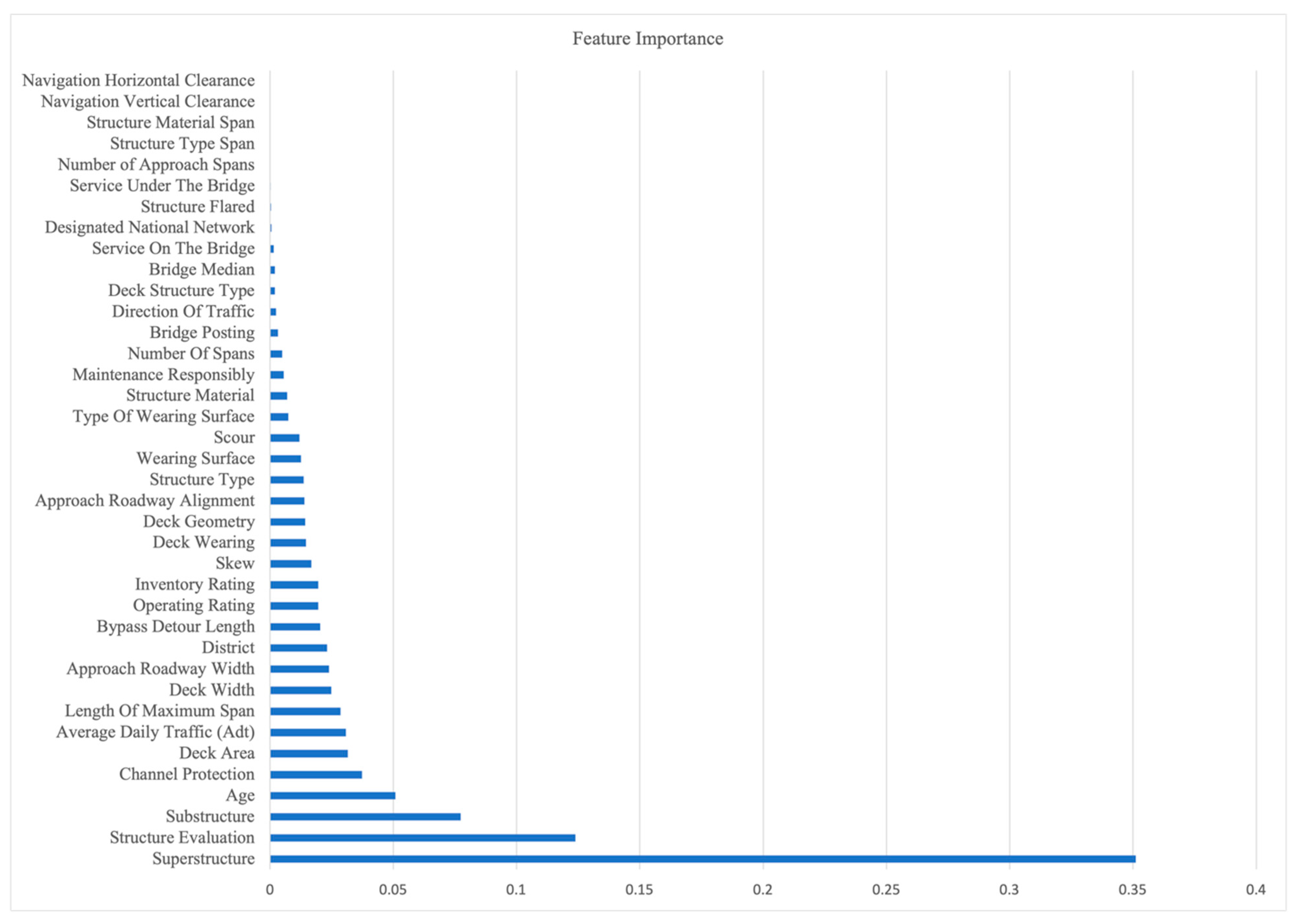
By developing the ML models, the Boruta algorithm has been used to determine whether or not the examined feature is correlated to deck conditions. As shown in Table 5, 27 out of the 38 input features were confirmed by Boruta, while 12 of the input features were rejected. Some features might have been rejected because of either poor relation or lack of relation with the output, or even because of the nature of the dataset. Due to the fact that Boruta does not provide evaluation measurements for each feature, XGboost and RF methods were used to determine the importance of each feature. By examining Figure 2 and Figure 3, it can be observed that the most highly related features between the two methods of XGboost and RF are the same, and all of them have been confirmed by the Boruta algorithms. This shows that the feature importance methods used in this research work properly. The XGboost algorithm gives a score between 0 to 900, where 0 represents the least correlated feature and 900 represents the highest correlated feature. In this research, features having a score of more than 100 are selected. Similarly, the RF algorithm gives a score between 0 to 0.4, where 0 represents the least correlated feature and 0.4 represent the highest correlated feature. In this research, features having a score of more than 0.2 are considered important features. Based on the results, it was determined that the top important features using the two methods of XGboost and RF include superstructure, substructure, deck wearing, age, district, ADT, channel protection, operating rating, structure evaluation, deck area, deck width, length of maximum span, and approach roadway width. On the other hand, features that received low scores include navigation, horizontal/vertical clearance, service on/under the bridge, structure flared, and the number of approaches spans. In addition, there are three differences between the feature importance as determined from XGboost and RF; for example, deck wearing, structure type and maintenance responsibility are considered among the top features based on XGboost, while bypass detour length, inventory rating, and skew have high importance based on RF.

The results of the completed feature selection process indicate that some of the selected features are consistent with previous research, such as age, ADT, deck area, operating rating, and length of the maximum span. However, features, such as approach roadway width, channel protection, and district, which are among the most relevant variables to deck condition based on the XGboost and RF feature selection, were not considered by previous research.

4.2. Machine Learning Outputs

Using the “optimal” features that were identified based on the three feature selection models, seven ML algorithms have been implemented to determine which ML algorithm has the highest accuracy for predicting deck conditions.

Before implementing the ML algorithms, their hyperparameters have been optimized using a grid search with 5-fold cross-validation. Due to the high number of possible combinations of hyperparameter ranges, the most common ranges have been analyzed. As shown in

Table 6. Hyperparameter Optimization.

Model	Hyperparameter	Analyzed Values	Model 1	Model 2	Model 3
kNN	K value	[1–40]	9	9	38
DT	max_depth	[non, 3–10]	5	7	7
	min_sample_split	[2, 5, 10]	2	2	10
	min_sample_leaf	[1, 2, 4]	2	2	1
XGboost	max_depth	[3–10]	6	6	6
	Learning_rate	[0.01–0.3]	0.1	0.1	0.1
	Gamma	[0–0.5]	0.2	0.2	0.2
	subsample	[0.5–1]	0.7	0.7	0.7
	Colsample_bytree	[0.5–0.9]	0.7	0.7	0.7
	Min_child_wieght	[1–5]	5	5	5
RF	max_depth	[5–15]	15	15	15
	N_estimators	[100, 200, 300]	300	300	300
	Class_wieght	[None, balanced]	None	None	None
	Random_state	42	42	42	42
LR	C	[0.1, 1, 10]	10	10	0.1
	Class_wieght	[None, balanced]	balanced	balanced	balanced
	Random-state	42	42	42	42
SVM	C	[0.1, 1, 10]	10	10	10
	Gamma	[0.1, 0.01, 0.001 ]	0.01	0.01	0.01
	Class_weight	[None, balanced]	None	None	None
	Kernel	[linear, rbf, sigmoid]	rbf	rbf	rbf
ANN	Number of hidden layers	[1, 2, 3, 4, 5]	6	6	5
	Number of neoruns	[1–10]	12	12	11
	Learning rate	[0.1, 0.01, 0.001, 0.001]	0.1	0.1	0.1
	Batch_size	[16, 32, 64, 128, 256]	32	32	32
	optimizer	[LBFGS, SGD, ADAM]	ADAM	ADAM	ADAM

, the optimal k value of the kNN algorithm for both XGboost (Model 1) and RF (Model 2) features selection models is 9, while the optimal k value is 32 when the most-common-feature model (Model 3) is used. All the optimal hyperparameters of XGboost and RF algorithms are the same for all three feature selection models. For the LR algorithm, while the optimal C value for Model 1 and Model 2 is 10, the optimal C is 0.1 in the case of Model 3. For the SVM algorithm, all the optimal hyperparameters are similar in all three feature selection models. For the ANN, only the optimal number of hidden layers and the optimal number of neurons in case of Model 3 is different, with 5 layers and 11 neurons for each layer compared to Model 1 and Model 2 with 6 hidden layers and 12 neurons for each layer. For the DT algorithms, the optimal max_depth for Model 1 is 5, and 7 for Model 2 and model 3. Two samples were required to split an internal node and be at a leaf node for both Model 1 and Model 2, but Model 3 required 10 numbers for splitting in an internal node and one number to be at a leaf node.

The performance of each model was evaluated using the confusion matrix by six different validation metrics: (1) accuracy, (2) precision, (3) recall, (4) F1-score, (5) Cohen’s Kappa, and (6) average area under the precision-recall curve (AUC-PR) on both training and test datasets to avoid overfitting. These are the most common metrics for evaluating classifiers [43]. After cleaning the dataset, 18,969 records for concrete bridges in Ohio were used. A total of 80% of the dataset was used for training, and 20% for testing. All the classification models, including k-NN, ANN, SVM, LR, DT, RF, and XGboost, were implemented to identify the most accurate results.

Table 7. Model evaluation of deck condition prediction using XGboost feature selection (Model 1).

Model	Accuracy		Precision		Recall		F1-Score		Cohen’s Kappa		AverageAUCPR
	Train	Test	Train	Test	Train	Test	Train	Test	Train	Test	Train	Test
Single Models
k-NN	81.650	74.564	81.847	75.006	81.650	74.564	81.669	74.589	75.848	66.486	85.974	80.543
ANN	87.930	85.943	87.989	86.009	87.930	85.943	87.906	85.928	84.246	81.697	94.419	92,529
LR	85.834	84.899	85.959	85.058	85.834	84.899	85.828	85.058	81.516	80.368	93.391	92.998
SVM	86.651	85.568	86.793	85.761	86.651	85.568	86.645	85.572	82.579	81.227	93.727	93.231
DT	86.946	85.836	87.064	86.030	86.946	85.836	86.933	85.829	82.985	81.608	93.878	93.447
Ensemble Models
XGboost	91.210	86.827	91.217	86.872	91.210	86.827	91.198	86.819	88.494	82.818	96.084	93.505
RF	95.802	86.586	95.824	86.692	95.802	86.586	95.805	86.589	94.494	82.524	98.195	92.467

,

Table 8. Model evaluation of deck conditions prediction using RF feature selection (Model 2).

Model	Accuracy		Precision		Recall		F1-Score		Cohen’s Kappa		AverageAUCPR
	Train	Test	Train	Test	Train	Test	Train	Test	Train	Test	Train	Test
Single Models
k-NN	83.873	78.902	86.026	79.143	83.873	78.902	83.902	78.930	78.818	72.285	89.773	87.262
ANN	87.561	85.944	87.611	86.010	87.561	85.943	87.551	85.929	83.756	81.693	94.085	93.325
LR	86.0623	85.327	86.185	85.497	86.062	85.327	86,056	85.330	81.810	80.918	93.455	93.106
SVM	86.591	85.568	86.735	85.751	86.591	85.568	86.585	85.571	82.503	81.226	93.686	93.217
DT	87.916	85.970	88.023	86.088	87.916	85.970	87.913	85.968	84.208	81.726	94.150	93.359
Ensemble Models
XGboost	90.929	86.639	90.933	86.708	90.929	86.639	90.916	86.633	88.127	82.591	95.993	93.437
RF	95.521	86.265	95.548	86.377	95.521	86.265	95.522	86.270	94.125	82.112	97.999	92.293

and

Table 9. Model evaluation of deck conditions prediction using most common features (Model 3).

Model	Accuracy		Precision		Recall		F1-Score		Cohen’s Kappa		AverageAUCPR
	Train	Test	Train	Test	Train	Test	Train	Test	Train	Test	Train	Test
Single Models
k-NN	50.394	45.809	50.058	44.0189	50.394	45.809	48.913	44.0189	32.479	26.100	62.504	59.269
ANN	48.011	47.389	48.060	45.713	48.011	47.389	46.539	45.533	31.319	28.223	60.554	58.985
LR	31.429	32.904	35.786	37.451	31.429	32.904	30.451	31.961	16.150	17.953	61.993	63.889
SVM	46.063	45.781	46.327	43.724	46.063	45.783	42.063	41.515	24.631	24.379	58.200	57.381
DT	49.538	45.783	49.734	44.601	49.538	45.873	47.730	43.621	30.941	25.722	60.755	58.249
Ensemble Models
XGboost	62.839	49.531	64.835	48.533	62.839	49.531	62.038	47.595	49.522	31.072	74.239	60.904
RF	87.575	49.933	88.588	48.702	87.575	49.933	87.506	48.110	83.419	31.764	88.821	60.502

summarize the ML algorithms’ deck condition prediction results when the different sets of features were utilized.

Table 7 shows the results when XGboost feature selection (Model 1) was used. As shown in Table 7, it was determined that, in general, the ensemble models exhibited better performance compared to the single models. While the RF algorithm could achieve the highest performance in terms of training sets (accuracy = 95.521%, kappa = 94.494%, AUC-PR = 98.195%), the XGboost algorithm, on an unseen dataset, could achieve the best performance (accuracy = 86.639%, kappa = 88.494%, AUC-PR = 93.505%). In terms of the training dataset, the RF model exhibited the highest accuracy (accuracy = 95.802%), and the level of agreement between predicted and actual samples was significant (kappa = 94.494%) with perfect precision and recall (AUC-PR = 92.467%). Having high performance in the training dataset demonstrates that the model has learned the pattern adequately and is able to make accurate predictions on an unseen dataset. On the test dataset, the XGboost model could classify the majority of the samples adequately (accuracy = 86.827%), and it performed well in terms of precision, recall, and F1-score (precision = 86.872%, recall = 86.827%, F1-Score = 86.819%). It also demonstrated excellent performance in terms of the trade-off between precision and recall (AUC-PR = 93.505%). A high kappa value (k = 82.818) indicates an acceptable agreement between predicted and actual classes. Generally, the XGboost model exhibited reasonable performance. It is worth mentioning that both XGboost and RF models could achieve significant performance in both training and test sets. Among the single algorithms, the ANN and DT models achieved the best performance in terms of test and training sets. It should be noted that while XGboost and RF algorithms as ensemble models showed the highest accuracy, ANN, DT, SVM, and LR models could predict deck condition with acceptable performance. The kNN exhibited the poorest performance among all the algorithms that were used (accuracy = 74.564%, precision = 75.006%, recall = 74.564%, F1-Score = 74.589%, kappa = 66.486%, AUC-PR = 80.543%).

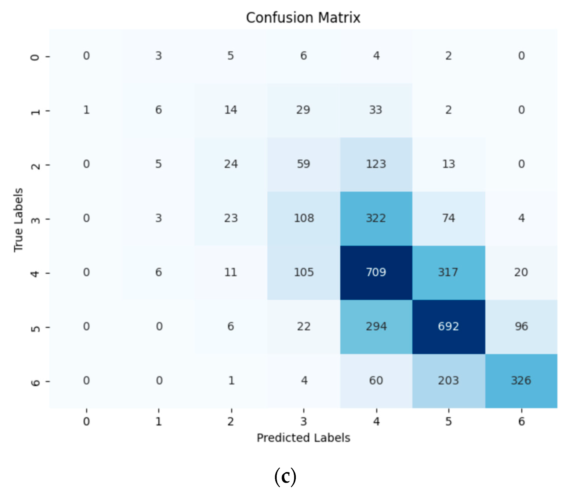
Table 8 shows the results when RF feature selection (Model 2) was used. Similar to Model 1, ensemble models including RF and XGboost, respectively, could achieve the highest prediction performance on the training and test datasets. All the evaluation metrics for the RF algorithm on the training dataset were larger than 94%. On the test dataset, the XGboost model achieved more than 86% accuracy, recall, precision, and F1-score, and more than 93% of AUC-PR could produce a significant prediction. Among single models, similar to Model 1, the ANN, DT, SVM, and LR models exhibited an acceptable performance, and kNN achieved the lowest accuracy. For further visualization of the results, the confusion matrices of the RF algorithms corresponding to the three feature selection models are shown in Figure 4a–c as an example. In these confusion matrices, the rows represent the true deck condition, and the columns indicate the predicted deck conditions.

Table 9 shows the results of the ML algorithms when only the “most common” features were used as input for the prediction algorithm (Model 3). As shown in Table 9, none of the ML algorithms were able to achieve more than 50% accuracy in the test group set, which indicates that the models are not able to classify the data properly. Furthermore, less than 65% AUC-PR for all the evaluation metrics indicates that poor performance between precision and recall occurred. The RF model was able to achieve the highest performance with (accuracy = 49.933%, precision = 48.702%, recall = 49.933%, F1-score = 48.110%, kappa = 31.764%, AUC-PR = 60.502%), XGboost had the second best performance (Accuracy = 49.521%, Precision = 48.533%, Recall = 49.531%, F1-Sscore = 47.595%, kappa = 31.072%, AUC-PR = 60.904%), and the ANN, DT, kNN, SVM and LR models’ performances were lower. This confirms the research hypothesis that the use of features that may have worked well in previous research studies on different locations does not necessarily guarantee the adequacy of their use in other locations. Thus, DOTs in different geographic locations need to conduct a feature-selection analysis to best select the related features which are specific to their own dataset. This validates the usefulness of the proposed framework.

In comparison to other studies, obtaining more than 93% AUC-PR, and 86% accuracy for XGboost and RF models, as well as more than 92% AUC-PR and 85% accuracy for ANN, SVM, and LR is acceptable for predicting deck condition. Previous studies such as Assad et, al. [8], Nguyen and Dinh [13], and Liu et al. [48], were able to achieve similar accuracies. However, they used different datasets corresponding to other states. The model which has been developed by this study can assist ODOT in predicting the future deck condition of bridges accurately, and transportation agencies will be able to save time and money when making informed decisions about their maintenance priorities.

5. Discussion

As discussed previously, every dataset will have some common and some unique features depending on the location of the dataset, weather, service type, nature of the data, etc. We can identify, from the features importance models implemented by this research, which features have the most significant effects on the deterioration of bridges in Ohio. Features such as deck area, deck width, length of maximum span, and approach roadway width relate to the geometry of the bridge, while features such as superstructure, substructure, channel protection, operating rating, and structure evaluation reflect the importance of core elements of bridges. Deck wearing and ADT can be related to the volume of traffic on Ohio bridges. The district is another factor to consider for predicting deck conditions, and it can also be interpreted that the location of the bridge has a significant effect on the condition of the bridge and can be related to the weather or the volume of traffic. Additionally, the age of the bridge is another important feature that has been considered in many previous research studies. It is worth mentioning that features such as approach roadway width, channel protection, and district are not collected by other states. Similarly, other scholars have found unique features based on their datasets, as illustrated in Table 3, such as wearing surface, rib flange, and skew angle [2,8,13]. Therefore, we can conclude that the set of important features for predicting bridge conditions may vary between locations because geographic variations, such as temperature, average daily traffic, and environmental conditions, can significantly affect the optimal features that should be used in ML models for predicting the deck condition.

This research conducted a comprehensive comparison of machine learning algorithms for predicting deck conditions. Since this study looked for the most accurate results, the most common ML models have been implemented, including artificial neural networks (ANN), k-nearest neighbors (k-NN), decision tree (DT), eXtreme gradient boosting (XGboost), logistic regression (LR), random forest (RF), and support vector machine (SVR). Different evaluation metrics including accuracy, precision, recall, F1-score, Cohen’s kappa, and AUC-PR have been utilized to evaluate and compare the ML model. As illustrated in Table 7 and Table 8, and after optimizing the hyperparameters, results indicate that ensemble algorithms such as XGboost and RF achieved more than 92% AUC-PR, 86% accuracy and 82% kappa, and were the most accurate algorithms to predict the deck conditions. In terms of the training sets, RF achieved more than 92% accuracy in all the evaluation metrics, which was significant. However, the kNN model achieved the lowest performance when both the RF and XGboost feature-selection models were used, with less than 80% accuracy and less than 80% kappa. It should be noted that single models such as ANN, DT, LR, and SVM achieved more than 92% AUC-PR and more than 85% accuracy, which is an acceptable performance. Table 7 and Table 8 demonstrate that XGboost feature selection (Model 1) and RF feature selection (Model 2) performed well and they produced very similar results in both training and test datasets using seven different ML algorithms; however, XGboost feature selection generally demonstrated slightly better performance compared to the RF feature selection model. As shown in Table 9, ML algorithms were not able to predict deck conditions properly when the “most common” features (Model 3) was used. The accuracies of all seven ML algorithms using Model 3 were less than 50%, which indicates that the algorithms were not able to classify unseen datasets properly, and the fact that all of the evaluation metrics were less than 30% kappa indicates a poor level of agreement between predicted and actual classes. Additionally, having less than 61% AUC-PR for all the ML algorithms demonstrates a poor trade-off between precision and recall.

It is important to compare the performance of ML models for different reasons. Firstly, it allows us to compare all ML models and achieve the best performance for predicting the deck conditions. Additionally, it is helpful for future research. Moreover, using both ensemble and single algorithms enhances researchers’ understanding of the strengths and limitations of different models, and also enables them to analyze these models individually to discern their specific characteristics and hyperparameters. The proposed approach provides valuable insight for future research to improve the understanding of various ML models. It should be noted that the fact that XGboost and RF algorithms achieved the best results in this research does not necessarily mean that they are the best algorithms to use in other locations. Since all the algorithms achieved a fair accuracy and were implemented in a very short time, selecting the best algorithm based on the characteristics of the data and strengths of the algorithms, as discussed in Section 2.2, is recommended for every project, to achieve the most accurate results.

Findings from this research will enhance researchers’ understanding of the most significant parameters that can affect the deterioration of a bridge’s deck, specifically in the state of Ohio. This research represents an application of ML models on the ODOT dataset to predict bridges’ deck conditions and provides valuable insight for future research. It helps scholars to choose the best ML algorithms for their future works, with the most optimized hyperparameters. Additionally, it indicates that different locations may have different important features in the prediction of the deterioration of a bridge’s deck. This research also enhances agencies’ perspectives on the overall performance and general life expectancy of bridges using machine learning. Such knowledge may help bridge owners be proactive in terms of planning maintenance and replacement activities. The information obtained from this research may be useful for planning purposes during the development of Capital Improvement Program plans, to ensure the proper and effective distribution of funds allocated for the maintenance, rehabilitation, and repair of bridges.

6. Conclusions

Decks are the most vulnerable part of bridges, and their exposure to damage will incur a significant maintenance expense. For this reason, it is important to be able to predict deck conditions accurately and to effectively allocate resources for repair and maintenance activities when needed. The research described in this paper proposed a framework for optimizing the use of machine learning (ML) algorithms to predict bridge deck deterioration more accurately. The framework first determines “optimal” features that can be related to deck deterioration conditions using XGboost and random forest feature-selection methods. The framework then proposes the use of different ML algorithms based on the “optimal” features to select the most accurate algorithm. Based on the research findings, the following conclusions can be made:

• XGboost and RF feature selection models could adequately select optimal features with very similar results; however, XGboost feature selection (Model 1) generally demonstrates slightly better performance compared to RF (Model 2).
• Seven machine learning algorithms, including artificial neural networks (ANN), k-nearest neighbors (k-NN), decision tree (DT), eXtreme gradient boosting (XGboost), logistic regression (LR), random forest and support vector machine (SVR), have been implemented to classify deck conditions. Findings from this research showed that ensemble ML models are more accurate than single models. XGboost and RF algorithms with 93% and 92% AUC-PR, respectively, could have an excellent trade-off between precision and recall, as well as more than 86% accuracy for both algorithms, indicating a satisfactory classification strength. However, single models such as kNNs, that could achieve less than 80% accuracy and less than 88% AUC-PR in both XGboost and RF feature selection models, were not as accurate as ensemble models.
• This research demonstrates that ML algorithms using the most common features (Model 3) were not able to classify datasets properly, with less than 50% accuracy and less than 30% kappa when all seven ML algorithms were used.
• It has been concluded that every dataset in each geographic location needs a separate analysis to select the features that most impact deck conditions. It is suggested that each DOT needs to conduct a separate feature-selection analysis for their own datasets to determine the most important features.

It has been concluded that the framework that has been proposed in the paper could predict deck condition deterioration with acceptable accuracy using ML algorithms, provided that the optimal features are used as input to the algorithms. Therefore, this research can serve as a valuable resource to help various agencies allocate their budgets efficiently and obtain the most accurate measurements for future bridges. Future work can further investigate the reasons why different features have been selected by different scholars, and can also implement the proposed prediction framework to predict the future condition of other bridge components such as the superstructure and substructure.

References

- Martinez, P.; Mohamed, E.; Mohsen, O.; Mohamed, Y. Comparative study of data mining models for prediction of bridge future conditions. J. Perform. Constr. Facil. 2020, 34, 04019108. [Google Scholar] [CrossRef]
- Ilbeigi, M.E.; Ebrahimi Meimand, M. Statistical forecasting of bridge deterioration conditions. J. Perform. Constr. Facil. 2020, 34, 04019104. [Google Scholar] [CrossRef]
- O. (Ohio D. of Transportation), “AssetWise”, 2021. Available online: https://www.transportation.ohio.gov/working/data-tools/resources/assetwise-inspection-system. (accessed on 1 January 2021).
- Bhalla, D. Select Important Variables Using Boruta Algorithm; TechTarget: Boston, MA, USA, 2017. [Google Scholar]
- Manafpour, A.; Guler, I.; Radlińska, A.; Rajabipour, F.; Warn, G. Stochastic analysis and time-based modeling of concrete bridge deck deterioration. J. Bridge Eng. 2018, 23, 04018066. [Google Scholar] [CrossRef]
- Chang, M.; Maguire, M.; Sun, Y. Stochastic modeling of bridge deterioration using classification tree and logistic regression. J. Infrastruct. Syst. 2019, 25, 04018041. [Google Scholar] [CrossRef]
- Saeed, T.U.; Qiao, Y.; Chen, S.; Gkritza, K.; Labi, S. Methodology for probabilistic modeling of highway bridge infrastructure condition: Accounting for improvement effectiveness and incorporating random effects. J. Infrastruct. Syst. 2017, 23, 04017030. [Google Scholar] [CrossRef]
- Assaad, R.; El-adaway, I.H. Bridge infrastructure asset management system: Comparative computational machine learning approach for evaluating and predicting deck deterioration conditions. J. Infrastruct. Syst. 2020, 26, 04020032. [Google Scholar] [CrossRef]
- Karan, E.; Mansoob, V.K.; Khodabandelu, A.; Asgari, S.; Mohammadpour, A.; Asadi, S. Using Artificial Intelligence to Automate the Quantity Takeoff Process. In Proceedings of the International Conference on Software Business Engineering, Amsterdam, The Netherlands, 29 May 2021; pp. 13–14. [Google Scholar]
- Huang, Y.H. Artificial neural network model of bridge deterioration. J. Perform. Constr. Facil. 2010, 24, 597–602. [Google Scholar] [CrossRef]
- Srikanth, I.; Arockiasamy, M. Deterioration models for prediction of remaining useful life of timber and concrete bridges: A review. J. Traffic Transp. Eng. 2020, 7, 152–173. [Google Scholar] [CrossRef]
- Agrawal, A.K.; Kawaguchi, A.; Chen, Z. Deterioration rates of typical bridge elements in New York. J. Bridge Eng. 2010, 15, 419–429. [Google Scholar] [CrossRef]
- Nguyen, T.T.; Dinh, K. Prediction of bridge deck condition rating based on artificial neural networks. J. Sci. Technol. Civ. Eng. (STCE)-HUCE) 2019, 13, 15–25. [Google Scholar] [CrossRef] [Green Version]
- Lu, P.; Wang, H.; Tolliver, D. Prediction of bridge component ratings using ordinal logistic regression model. Math. Probl. Eng. 2019, 2019, 9797584. [Google Scholar] [CrossRef] [Green Version]
- Lim, S.; Chi, S. Xgboost application on bridge management systems for proactive damage estimation. Adv. Eng. Inform. 2019, 41, 100922. [Google Scholar] [CrossRef]
- Abedin, M.; Mokhtari, S.; Mehrabi, A.B. Bridge damage detection using machine learning algorithms. In Health Monitoring of Structural and Biological Systems XV; SPIE: Online, 2021; Volume 11593, pp. 532–539. [Google Scholar]
- O’Connor, A.J.; Sheils, E.; Breysse, D.; Schoefs, F. Markovian bridge maintenance planning incorporating corrosion initiation and nonlinear deterioration. J. Bridge Eng. 2013, 18, 189–199. [Google Scholar] [CrossRef]
- Wellalage, N.K.; Zhang, T.; Dwight, R. Calibrating Markov chain–based deterioration models for predicting future conditions of railway bridge elements. J. Bridge Eng. 2015, 20, 04014060. [Google Scholar] [CrossRef] [Green Version]
- Ranjith, S.; Setunge, S.; Gravina, R.; Venkatesan, S. Deterioration prediction of timber bridge elements using the Markov chain. J. Perform. Constr. Facil. 2013, 27, 319–325. [Google Scholar] [CrossRef]
- Sadat-Mohammadi, M.; Nazari-Heris, M.; Ameli, A.; Asadi, S.; Mohammadi-Ivatloo, B.; Jebelli, H. Application of Machine Learning for Predicting User Preferences in Optimal Scheduling of Smart Appliances. In Application of Machine Learning and Deep Learning Methods to Power System Problems; Springer: Cham, Switzerland, 2021; pp. 345–355. [Google Scholar]
- Gao, C.; Elzarka, H. The use of decision tree based predictive models for improving the culvert inspection process. Adv. Eng. Inform. 2021, 47, 101203. [Google Scholar] [CrossRef]
- Mousavi, M.; Ayati, M.; Hairi-Yazdi, M.R.; Siahpour, S. Robust Linear Parameter Varying Fault Reconstruction of Wind Turbine Pitch Actuator using Second-order Sliding Mode Observer. J. Electr. Comput. Eng. Innov. 2023, 11, 229–241. [Google Scholar]
- Siahpour, S.; Ayati, M.; Haeri-Yazdi, M.; Mousavi, M. Fault detection and isolation of wind turbine gearbox via noise-assisted multivariate empirical mode decompositi on algorithm. Energy Equip. Syst. 2022, 10, 271–286. [Google Scholar]
- Esteghamati, M.Z.; Flint, M.M. Developing data-driven surrogate models for holistic performance-based assessment of mid-rise RC frame buildings at early design. Eng. Struct. 2021, 245, 112971. [Google Scholar] [CrossRef]
- Abdelmalek-Lee, E.; Burton, H. A dual Kriging-XGBoost model for reconstructing building seismic responses using strong motion data. Bull. Earthq. Eng. 2023, 1–27. [Google Scholar] [CrossRef]
- Melhem, H.G.; Cheng, Y. Prediction of remaining service life of bridge decks using machine learning. J. Comput. Civ. Eng. 2003, 17, 1–9. [Google Scholar] [CrossRef]
- Soleimani, F.; Hajializadeh, D. Bridge seismic hazard resilience assessment with ensemble machine learning. In Structures; Elsevier: Amsterdam, The Netherlands, 2022; Volume 38, pp. 719–732. [Google Scholar]
- Zhang, W.; Zhang, R.; Wu, C.; Goh, A.T.; Lacasse, S.; Liu, Z.; Liu, H. State-of-the-art review of soft computing applications in underground excavations. Geosci. Front. 2020, 11, 1095–1106. [Google Scholar] [CrossRef]
- Taunk, K.; De, S.; Verma, S.; Swetapadma, A. A brief review of nearest neighbor algorithm for learning and classification. In Proceedings of the 2019 International Conference on Intelligent Computing and Control Systems (ICCS), Madurai, India, 15–17 May 2019; pp. 1255–1260. [Google Scholar]
- Bolourani, A.; Bitaraf, M.; Tak, A.N. Structural health monitoring of harbor caissons using support vector machine and principal component analysis. In Structures; Elsevier: Amsterdam, The Netherlands, 2021; Volume 33, pp. 4501–4513. [Google Scholar]
- Sarzaeim, P.; Bozorg-Haddad, O.; Bozorgi, A.; Loáiciga, H.A. Runoff projection under climate change conditions with data-mining methods. J. Irrig. Drain. Eng. 2017, 143, 04017026. [Google Scholar] [CrossRef]
- Mitchell, R.; Frank, E. Accelerating the XGBoost algorithm using GPU computing. PeerJ Comput. Sci. 2017, 3, e127. [Google Scholar] [CrossRef] [Green Version]
- Li, Z.; Liu, Z.; Ding, G. Feature selection algorithm based on XGBoost. J. Commun. 2019, 40, 101. [Google Scholar]
- Breiman, L. Random forests. Mach. Learn. 2001, 45, 5–32. [Google Scholar] [CrossRef] [Green Version]
- Demolli, H.; Dokuz, A.S.; Ecemis, A.; Gokcek, M. Wind power forecasting based on daily wind speed data using machine learning algorithms. Energy Convers. Manag. 2019, 198, 111823. [Google Scholar] [CrossRef]
- Chakraborty, D.; Elzarka, H. Advanced machine learning techniques for building performance simulation: A comparative analysis. J. Build. Perform. Simul. 2019, 12, 193–207. [Google Scholar] [CrossRef]
- Auria, L.; Moro, R.A. Support Vector Machines (SVM) as a Technique for Solvency Analysis; Elsevier: Amsterdam, The Netherlands, 2008. [Google Scholar]
- Kutty, A.A.; Wakjira, T.G.; Kucukvar, M.; Abdella, G.M.; Onat, N.C. Urban resilience and livability performance of European smart cities: A novel machine learning approach. J. Clean. Prod. 2022, 378, 134203. [Google Scholar] [CrossRef]
- Esteghamati, M.Z.; Flint, M.M. Do all roads lead to Rome? A comparison of knowledge-based, data-driven, and physics-based surrogate models for performance-based early design. Eng. Struct. 2023, 286, 116098. [Google Scholar] [CrossRef]
- Ren, J.; Zhang, B.; Zhu, X.; Li, S. Damaged cable identification in cable-stayed bridge from bridge deck strain measurements using support vector machine. Adv. Struct. Eng. 2022, 25, 754–771. [Google Scholar] [CrossRef]
- Sadat-Mohammadi, M.; Nazari-Heris, M.; Nazerfard, E.; Abedi, M.; Asadi, S.; Jebelli, H. Intelligent approach for residential load scheduling. IET Gener. Transm. Distrib. 2020, 14, 4738–4745. [Google Scholar] [CrossRef]
- Sadat-Mohammadi, M.; Shakerian, S.; Liu, Y.; Asadi, S.; Jebelli, H. Non-invasive physical demand assessment using wearable respiration sensor and random forest classifier. J. Build. Eng. 2021, 44, 103279. [Google Scholar] [CrossRef]
- Ray, S. A quick review of machine learning algorithms. In Proceedings of the 2019 International Conference on Machine Learning, Big Data, Cloud and Parallel Computing (COMITCon), Faridabad, India, 14–16 February 2019; pp. 35–39. [Google Scholar]
- Wakjira, T.G.; Ibrahim, M.; Ebead, U.; Alam, M.S. Explainable machine learning model and reliability analysis for flexural capacity prediction of RC beams strengthened in flexure with FRCM. Eng. Struct. 2022, 255, 113903. [Google Scholar] [CrossRef]
- Wakjira, T.G.; Abushanab, A.; Ebead, U.; Alnahhal, W. FAI: Fast, accurate, and intelligent approach and prediction tool for flexural capacity of FRP-RC beams based on super-learner machine learning model. Mater. Today Commun. 2022, 33, 104461. [Google Scholar] [CrossRef]
- Hong, H.; Zhu, J.; Chen, M.; Gong, P.; Zhang, C.; Tong, W. Quantitative structure–activity relationship models for predicting risk of drug-induced liver injury in humans. In Drug-Induced Liver Toxicity; Humana: New York, NY, USA, 2018; pp. 77–100. [Google Scholar]
- Chemchem, A.; Alin, F.; Krajecki, M. Combining SMOTE sampling and machine learning for forecasting wheat yields in France. In Proceedings of the 2019 IEEE Second International Conference on Artificial Intelligence and Knowledge Engineering (AIKE), Sardinia, Italy, 3–5 June 2019; pp. 9–14. [Google Scholar]
- Liu, K.; El-Gohary, N. Ontology-based semi-supervised conditional random fields for automated information extraction from bridge inspection reports. Autom. Constr. 2017, 81, 313–327. [Google Scholar] [CrossRef]
Figure 1.
Research methodology.
Figure 2.
Feature Importance Using XGBoost (Model 1).
Figure 3.
Feature Importance Using RF (Model 2).
Figure 4.
(a) Confusion matrix of RF algorithms Model 1; (b) Confusion matrix of RF algorithms Model 2; (c) Confusion matrix of RF algorithms Model 3.