
Pattern-Moving-Based Partial Form Dynamic Linearization Model Free Adaptive Control for a Class of Nonlinear Systems

1
School of Automation and Electrical Engineering, University of Science and Technology Beijing, and The Key Laboratory of Knowledge Automation for Industrial Processes of Ministry of Education, Beijing 100083, China
2
School of Information Engineering, Jingdezhen University, Jingdezhen 333000, China
*
Author to whom correspondence should be addressed.
Actuators 2021, 10(9), 223; https://0-doi-org.brum.beds.ac.uk/10.3390/act10090223
Submission received: 4 July 2021
/
Revised: 31 August 2021
/
Accepted: 2 September 2021
/
Published: 5 September 2021
(This article belongs to the Special Issue Dynamics and Control of Robot Manipulators)
Abstract
:This work addresses a pattern-moving-based partial form dynamic linearization model free adaptive control (P-PFDL-MFAC) scheme and illustrates the bounded convergence of its tracking error for a class of unknown nonaffine nonlinear discrete-time systems. The concept of pattern moving is to take the pattern class of the system output condition as a dynamic operation variable, and the control purpose is to ensure that the system outputs belong to a certain pattern class or some desired pattern classes. The P-PFDL-MFAC scheme mainly includes a modified tracking control law, a deviation estimation algorithm and a pseudo-gradient (PG) vector estimation algorithm. The classification-metric deviation is considered as an external disturbance, which is caused by the process of establishing the pattern-moving-based system dynamics description, and an improved cost function is proposed from the perspective of a two-player zero-sum game (TP-ZSG). The bounded convergence of the tracking error is rigorously proven by the contraction mapping principle, and the validity of the theoretical results is verified by simulation examples.
1. Introduction
In the process of industrial production, there is a range of complex equipment, such as sintering machines, rotary kilns, blast furnaces, and so on. Due to the increase in complexity, such as nonlinearity, high order, large delay, time-varying, and parameter perturbation, it is very difficult to establish an accurate mathematical model [1]. To a certain extent, this kind of production system is mainly governed by the law of statistical moving rather than the existing Newton’s law of mechanics. A group of the same or similar system working conditions can produce the corresponding products with the same or similar quality index parameters [2].
A feasible method of system modeling and control is the pattern recognition technology for these considered systems [3], and most researchers’ practice is to design the corresponding model and controller according to the different pattern classes of the system working condition [4,5]. Different from the previous multi-controller model design method based on pattern classes, a novel pattern-moving-based system dynamics description method was proposed in [6]. Its basic idea is to take the pattern class as a moving variable, and this variable is mapped to a computable space by class centers [7], interval numbers [8], and cells [9] due to its lack of arithmetic operation attribute. One advantage of the system dynamics description method introduced in [6] is that it is robust to system parameter disturbance and measurement noise. Regarding robust control, a well-known method is sliding mode control [10,11,12], which has a good ability to deal with external disturbances and system uncertainties. In recent years, a series of important research achievements have been made in sliding mode control, and many improved methods have been proposed, such as global sliding mode control [13] and terminal sliding mode control [14]. Different from the methods proposed in [10,11,12,13,14], the pattern-moving-based system dynamics description method is able to eliminate the system disturbance in the process of pattern classification, as long as the influence of the disturbance on the output does not change the pattern class to which the output belongs. In the case of various metric methods of pattern class, the linear autoregressive model with exogenous input (ARX) or interval ARX (IARX) model has been established, and the minimum-variance-based controller [6], optimal controller [15], predictive controller [16], and state-feedback-based [7] controller have been designed. However, it is well known that it is not easy to identify the system model order and parameters. In addition, even if a pattern-moving-based mathematical prediction model such as ARX or IARX is proposed, it is always an approximation of the real plant, and the unmodeled dynamics of the system are inevitable. Therefore, it is of significance to propose a pattern-moving-based data-driven control (DDC) method and design a controller whose parameters are adjusted by adopting the online input/output (I/O) data and the offline historical data simultaneously.
The data-driven controller is designed directly depending on the offline or/and online I/O data, instead of the explicit mathematical model of the controlled plant [17]. Generally, DDC can be almost cataloged into the following classes according to the different ways in which the data are used: (1) adaptive dynamic programming [18] and iterative learning control [19] based on offline and online data; (2) iterative feedback tuning [20] and virtual reference feedback tuning [21] based on offline data; (3) traditional MFAC [17,22,23,24] based on online data. The traditional MFAC method does not use the state space model but puts forward new concepts such as pseudo-gradient (PG) vector or pseudo-partial derivative (PPD) to capture the dynamic characteristics of the controlled plant, and it designs the controller through the dynamic linearization data model of the controlled plant at each operating point. Thus far, three equivalent dynamic linearization data models have been proposed, i.e., PFDL, compact-form dynamic linearization (CFDL), and the full-form dynamic linearization (FFDL) data model. By setting input correlation and output correlation components with different memory lengths, the three kinds of data models are different equivalent descriptions of system evolution, and they have different dynamic description capabilities for the controlled plant. Recently, due to many advantages of the MFAC method, such as the fact that establishing a controller merely depends on the measurement I/O data, the monotonic convergence of tracking error, and the bounded-input bounded-output stability of the closed-loop system, it has achieved many application results in many fields, and a few examples are as follows: the MFAC-based fault-tolerant control [25]; sensorless brushless direct current motor based on MFAC [26]; multi-agent systems tracking control [27]; MFAC-based sliding mode control [28]; chemical process based on MFAC [29], etc.
However, although the traditional MFAC algorithms have good control qualities for single-input single-output (SISO), multiple-input single-output, and multiple-input multiple-output time-varying structures and parameters in nonlinear discrete-time systems, there are few reports on MFAC for single-input multiple-output (SIMO) nonlinear systems or systems where the desired exact value of the output target cannot be determined exactly. In view of this kind of nonlinear system, a P-PFDL-MFAC method is proposed in this work and it considers that the difference in the output between next time and the current time is related to the differences in inputs in a time window between the current time and a specific previous time. The length of the time window corresponds to the number of PG vector elements, which is also called the pseudo-order of the equivalent PFDL data model. This is the most significant difference between the method proposed here and the pattern-moving-based CFDL-MFAC (P-CFDL-MFAC) scheme in [30], which considered that the output difference between next time and the current time is only related to the input difference between the current time and the previous time. The control purpose of this kind of system is to make the system outputs belong to one or some specific pattern classes. The first contribution of this work is to combine the pattern-moving-based system dynamics description with the traditional PFDL-MFAC method, and to design a control law algorithm based on two-player zero-sum game and saddle point theory [31,32] under the condition of classification-metric deviation. Another major contribution is that the bounded convergence of the tracking error dynamics of the closed-loop control system is rigorously proven by using the contraction mapping principle.
The remainder of this work is organized as follows. Section 2 introduces the preliminary of the work. Section 3 presents the problem formulation and designs a pattern-moving-based PFDL-MFAC scheme. The bounded convergence of the closed-loop system’s tracking error is proven in Section 4. Section 5 presents two simulation examples to demonstrate the correctness and efficiency of the proposed algorithms. A conclusion is given in Section 6.
Notation: denotes the real number domain; denotes the positive integer domain; is the real n-dimensional space; is the transpose of ; is the Euclidean norm, and is the consistent matrix norm.
2. Preliminary
Consider a class of SIMO nonaffine nonlinear discrete-time systems with unknown structure, order and parameters.
where ; denotes the output of and it satisfies ; is the whole system input and it satisfies ; , represent the unknown input and output orders, respectively, and they satisfy that , ; is the weak output measurement noise; denotes an unknown nonlinear discrete-time function; .
Assumption 1.
The input of this kind of system (1) is bounded, i.e., a constant exists and satisfies that .
A pattern-moving-based system dynamics description [6,7,8,9,30] that corresponds to system (1) is proposed in the following steps.
- (1)
- Feature extraction . A large number of inputs and outputs are collected offline, and the input data set and q-dimensional output vector set are obtained. Through the principal component analysis (PCA) feature extraction [33] of the output data, the first principal component information is obtained, and then the one-dimensional principal component information set will be obtained.
- (2)
- Classification and hybrid metrics . Using pattern classification technology to classify the first principal component information, the number of pattern classes , the class center value , and the class radius of each pattern class can be obtained, . Since the pattern class does not have the arithmetic operation attribute, the pattern class variable needs to be measured. Because the pattern class is a collection of pattern samples with the same or similar attributes, the method of combining the class center explicit metric and implicit metric is adopted, i.e., and . The implicit metric values are unknown, but there is a definite relationship between an implicit metric value and a class center explicit metric value, such as . The class center explicit metric represents the statistical attribute of the pattern class, while the implicit metric denotes the difference in each pattern sample in one pattern class.
- (3)
- Establishing the pattern-moving-based system dynamics equations. The inputs , implicit metric values , and class center explicit metric values are employed to construct the following dynamics equations.where is an unknown SISO nonlinear discrete-time system function; denote the input and output orders of system (2), respectively.
By choosing a reasonable classification method, such as a modified quantized control classification [34], it can be obtained that , which is named the class threshold. It exits a classification-metric deviation between the and , and , while . Let , then .
Remark 1.
As mentioned in the Introduction, the description of system dynamics based on pattern moving was first proposed in [6], and further studied in [7,8,9,30]. The basic idea is to treat the pattern class as a moving variable. Since this variable does not have the attribute of arithmetic operation, it is necessary to measure it into a computable space, and then construct the corresponding dynamic equation in this space. Obviously, the SISO nonlinear system or linear time-varying system can also be treated by the dynamic description method proposed in this section, but the feature extraction process is not required.
Remark 2.
The ultimate goal of classifying and measuring the first principal component information is to obtain a SISO system dynamics description in a computable space. From the perspective of pattern recognition technology, when the contribution rate of the first principal component obtained after feature extraction is more than , it is considered that the first principal component information does not lose the original information or it loses very little. If the contribution rate of the first principal component information does not reach , more principal component information should be considered. Then, after classification and class center explicit metric, the metric result of each pattern class variable is a vector. A pattern-moving-based SIMO system dynamics description is to be constructed in a computable space, but the output dimension may be less than that of the original system. For the pattern-moving-based SIMO system, its control method remains to be studied in the future. In this work, we only consider the case in which the contribution rate of the first principal component information is greater than .
3. Problem Formulation and Control Scheme
3.1. Problem Formulation
Through the above system dynamics description method, the model free adaptive tracking control problem of system (1) is transformed into the corresponding control problem of system (2) and (3). In order to carry out our next analysis, the following assumptions and lemma are proposed first.
Assumption 2.
The partial derivatives of nonlinear system function with respect to all variables of the system (2) exist and are continuous.
Assumption 3.
The system (2) satisfies the generalized Lipschitz condition, i.e.,
where , l denotes the input pseudo-order, which satisfies , and b is a positive constant.
Lemma 1
Because the implicit metric values are not available, the traditional MFAC methods can not be directly used in such systems. Therefore, this work will focus on the design of a new control scheme that merely depends on the obtained data , and the performance analysis of the closed-loop control system.
3.2. The P-PFDL-MFAC Scheme
It can be seen from the system dynamics Equations (2) and (3) that there is a classification-metric deviation between the initial predicted output and the final output of the system, and this deviation is always considered as a bounded external disturbance [12] in this work. Based on the saddle point theory of TP-ZSG proposed in [30,31,32], an improved cost function is designed in order to obtain a deviation estimation algorithm and an adaptive tracking control law, which aims to find an equilibrium point between the classification-metric deviation difference and the input difference. The basic idea is that even under large deviation fluctuation, a small input variation value can be found to optimize the loss function.
where ; is utilized to limit the variation in the control input difference, which satisfies ; denotes the desired class center explicit metric value at time instant ; is employed to limit the difference change in classification-metric deviation, which satisfies ; .
By solving the following equations
and
one has the optimal results, such as
and
where ; ; is a step-size, which satisfies and makes the control algorithm more general; .
In order to estimate the PG vector, the following objective function is designed.
where is a weight factor and it satisfies .
By letting
one can obtain the estimation algorithm of the PG vector as follows:
where ; is a step-size that satisfies and makes the estimation algorithm more general; .
Combining the above algorithms (6), (7), and (9), and proposing a reset algorithm of the PG estimation vector and a limitation mechanism of classification-metric deviation, the P-PFDL-MFAC scheme can be obtained.
where , , , , , , ; is the estimation vector of PG ; denotes a small positive constant; is the initial value of ; the algorithm (13) is the reset algorithm of the PG estimation vector, and the algorithm (14) denotes the limitation mechanism of classification-metric deviation.
It is known from the above algorithms that the PG estimation vector directly affects the quality of the control scheme. In order to enhance the time-varying parameters’ tracking ability for the PG estimation (10), it is necessary to add the reset algorithm (13). The limitation mechanism (14) is added to ensure that the deviation within one pattern class is not greater than the corresponding pattern class radius. The pseudo-order l is supposed to be less than or equal to the sum of the input and output orders . A large number of experiments show that the lower the system complexity, the smaller the value of l can be. On the contrary, the higher the system complexity, the greater the l should be. It is obvious that the proposed P-PFDL-MFAC algorithms in this work degenerate to the P-CFDL-MFAC algorithms designed in [30] when .
4. Performance of the Closed-Loop System
The focus of this section is to analyze the performance of the closed-loop tracking control system, i.e., to prove the tracking error bounded stability of the closed-loop control system. Before this, the following assumptions and lemmas are proposed.
Assumption 4.
Considering the nonlinear system (2), for any desired bounded output , a bounded input always exists and it can make the system output equal to .
Assumption 5.
The signal of the first element of the PG vector is assumed to be known and unchanged at any time k with , i.e., (or ), ϵ is a small positive constant. In this work, in order to simplify the derivation of the conclusion, it is always assumed that without loss of generality.
Lemma 2
If , then , where is the spectral radius of A.
Lemma 3
([17]). Let . For any given , there exists an induced consistent matrix norm such that where has the same meaning as Lemma 2.
It is known to all that Assumption 4 is a necessary condition for the design and solution of the control problem, and it also shows that the output of the system (2) is controllable. Many plants satisfy the condition of Assumption 5 to some extent, and its actual physical background is also very clear, i.e., the plant’s output increasing or decreasing corresponds to the control input increasing or decreasing. Next, our main results will be proven.
Lemma 4.
Proof of Lemma 4.
Taking the norm on both sides of (15) and using Lemma 1, yields
Square the first term on the right of (16) and obtain the following inequality:
Since and , it can be obtained that and it is obvious that . Thus, there must exist a constant that satisfies . It can be further deduced that
In view of (18), is bounded, since is bounded; thus, is bounded. □
Theorem 1.
For system (2) and (3) using the P-PFDL-MFAC scheme (10)–(14) under Assumptions 3–6 with the desired signal , if the controller parameters meet the following conditions
- (1)
- letting and ;
- (2)
- letting and , ;
- (3)
- letting , and there exists a such that ,
then the closed-loop control system guarantees that
where M is a constant and .
Proof of Theorem 1.
Substituting the classification-metric deviation estimation algorithm (11) into control algorithm (12), one has
Given , , , Equation (19) can be written as
where , .
Since , and , thus . It is known from Lemma 4 that is bounded and noted that ; here, is a positive constant. Given , , , , , , , there exist bounded constants , such that the following inequalities (21)–(25) hold when .
Letting and using inequality , one obtains
Letting and choosing , one has
Defining tracking error and letting
the control algorithm (12) can be written as
where . The secular equation of is
From Lemma 2 and inequality (25), one has and obtains
Further, it can be deduced that . From Lemma 3, one can obtain . According to the definition of , it is clear that . Letting and taking the norm on both sides of (27), one obtains
From Lemma 1 and Equation (27), one has
Choosing a reasonable , one can obtain
From the above inequality and , taking the norm on both sides of the Equation (29), one obtains
Letting , it is clear that . The inequality (31) can be recorded as
Letting
it is obvious that . One can see that if is bounded, then is bounded.
Next, the boundedness of will be proven.
Note that . Since , one obtains
Since , by choosing the reasonable , it exits and one obtains
It is clear that is bounded convergent; thus, the tracking error is bounded convergent, i.e., , M is a positive constant. □
Remark 3.
The contraction mapping principle is utilized to prove the bounded convergence in this work, and many inequalities are employed to handle the mapping relationships in Lemma 4 and Theorem 1. A critical technique is to let λ, γ, and take reasonable values that can guarantee the existence of constants , , , , , , , , , , , , and to make the inequalities used in the above derivations hold.
Remark 4.
It is obvious that the desired tracking target is an arbitrary bounded constant in Theorem 1. In fact, for the closed-loop control system based on pattern moving, the desired tracking target should be one or some specific pattern classes (), i.e., one or some specific pattern class centers (, ). Therefore, instead of focusing on each specific value of the system output, the P-PFDL-MFAC method focuses on whether the system outputs belong to one or some specific pattern classes, and this is the most significant difference between the method designed in this work and the model free adaptive quantization control method proposed in [35,36]. From this point of view, under the control input and output disturbance, even if the implicit metric value of the pattern class to which the system outputs belong satisfies when the desired target , it is still considered that the system’s tracking error is zero.
Remark 5.
The designed P-PFDL-MFAC method is employed for the considered system (2) and (3), which corresponds to a practical SIMO system (1). When the system is under the control input at time instant k, the output vector is obtained, and then is obtained by feature extraction , pattern classification , the class center explicit metric with the real-time output data , and a large amount of offline historical data. Generally speaking, the P-PFDL-MFAC method can be considered a novel data-driven method based on offline historical data and online real-time data, and this is a major difference from the traditional MFAC methods.
5. Simulation
Two examples are given to demonstrate the feasibility and effectiveness of the achieved algorithms in this section. In the simulation example of reference [37], the speed control of a Stanford manipulator’s joint 4 proposed in [38] was discussed. It considered that the controlled object is a discrete-time system with jump parameters while the load changes. In the first example below, this discrete-time system is also taken as the consideration object, and the designed P-PFDL-MFAC scheme is implemented. Example 2 is a SIMO nonlinear discrete-time numerical case. In this simulation case, the designed control scheme is adopted, and the control effects with different pseudo-orders are compared.
Example 1.
Consider a SISO discrete-time system with jump parameters
where is the system output, which denotes the speed of a Stanford manipulator’s joint 4; is the system input, which denotes the motor’s voltage and satisfies ; denotes the system random noise and it satisfies that ; is considered as a constant and ; is also a constant and ; the other two system jump parameters are as follows:
and
The control goal of our designed scheme is that the outputs belong to one or some special pattern classes, which is the most significant difference from the simulation in [37]. Firstly, a large number of outputs obtained under effective control inputs are divided into several pattern classes. Then, one or some desired pattern classes are taken as the targets of system control.
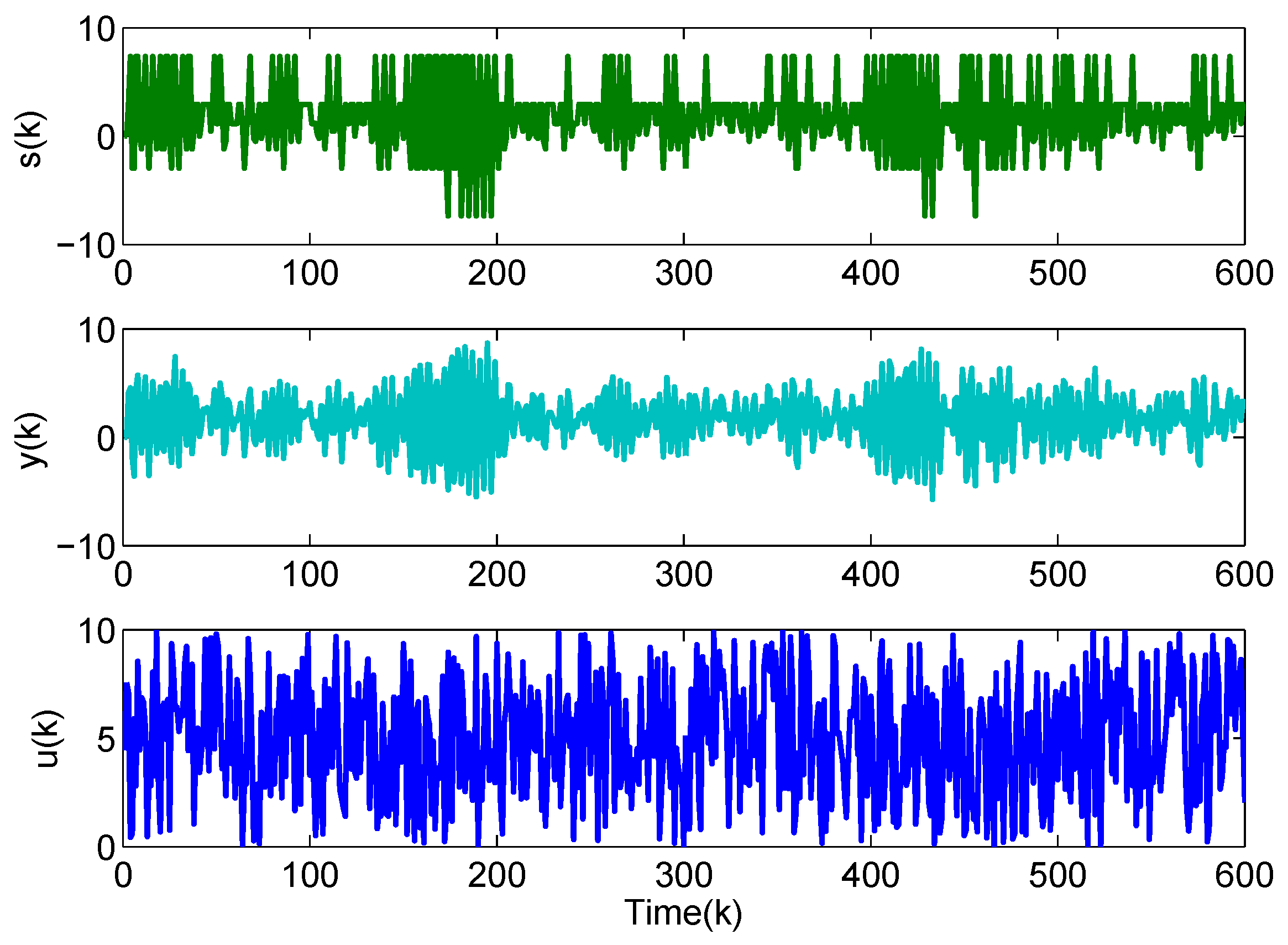
Step 1: Classification () and metrics () of massive offline data. Here, 600 evenly distributed inputs are taken and the corresponding outputs are obtained. A modified quantized control classification and class center explicit metric method (, ) [34] is adopted and described as follows.
where ; ; ; ; ; ; ; is the maximum working range of ; N denotes the number of pattern classes; .
Given the upper limit of the initial class radius at the working point 0 and other parameters such as and , one can obtain , and the output sequence is divided into segments. Furthermore, , , and class threshold can be obtained, respectively, . The parameter settings of the adopted classification method are , , . The distribution curves of , , and are shown in Figure 1. Table 1 shows the property values of each pattern class.
Remark 6.
To the best of our knowledge, there are many clustering and classification algorithms in statistical pattern recognition, such as ISODATA, K-means, C-means, and so on. A class center explicit metric and modified quantized control classification method is adopted in this work. As mentioned in [2], the product quality is directly related to the working conditions. Therefore, the parameter settings of condition classification are determined by the result of product quality clustering. Here, it is assumed that the first principal component information corresponds to good product quality, so the initial parameters (, , ) are configured to ensure that the working condition data belong to one pattern class.
Step 2: A pattern-moving-based system dynamics description is established with the obtained property values and data sets , , and .
where is an unknown nonlinear system function; denote the unkown input and output orders of , respectively.
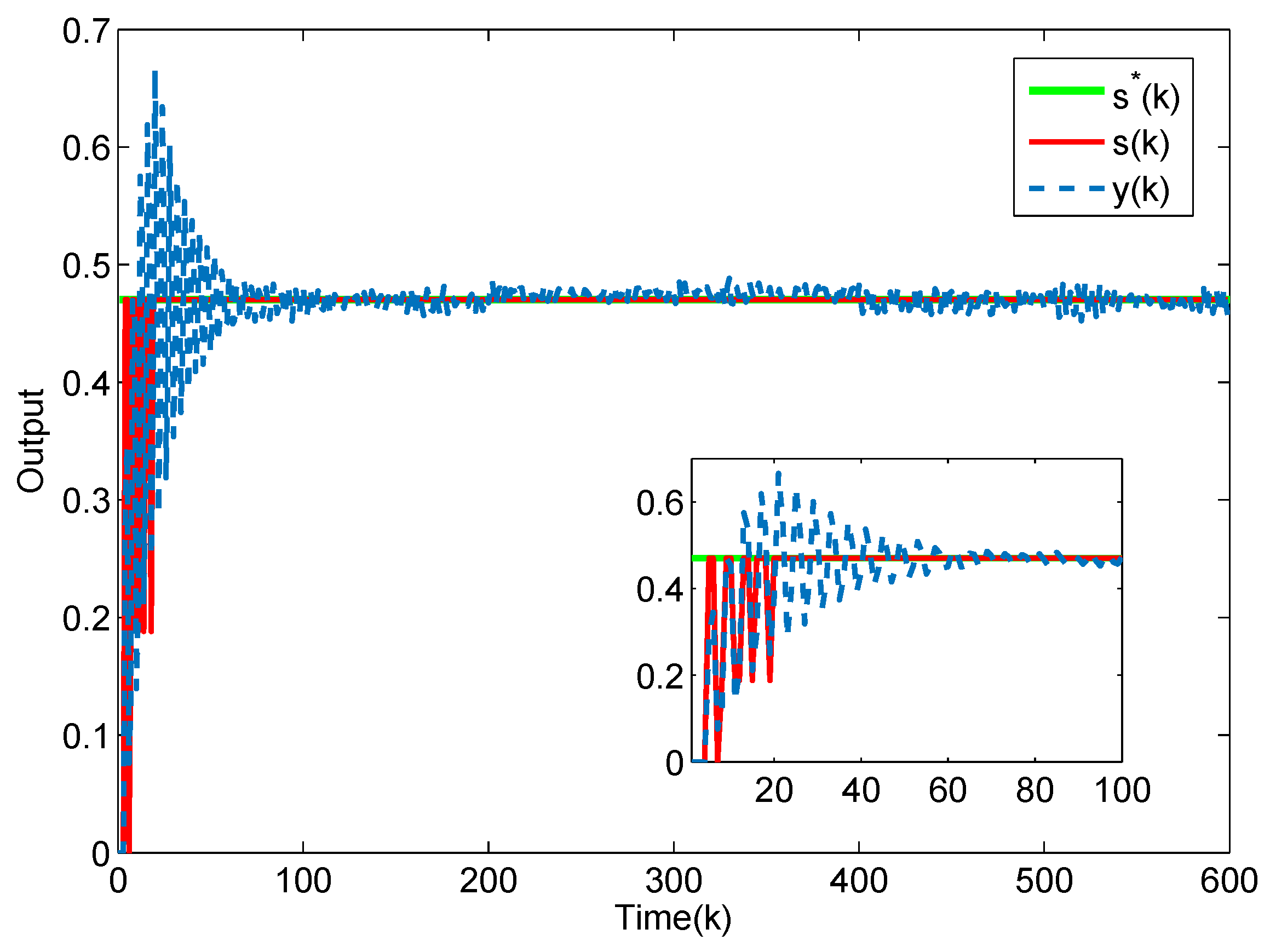
Step 3: Application of the control scheme. Nine pattern classes are obtained and the designed P-PFDL-PMFAC scheme (10)–(14) is employed to track the following targets.
where denotes that the object is pattern class 8.
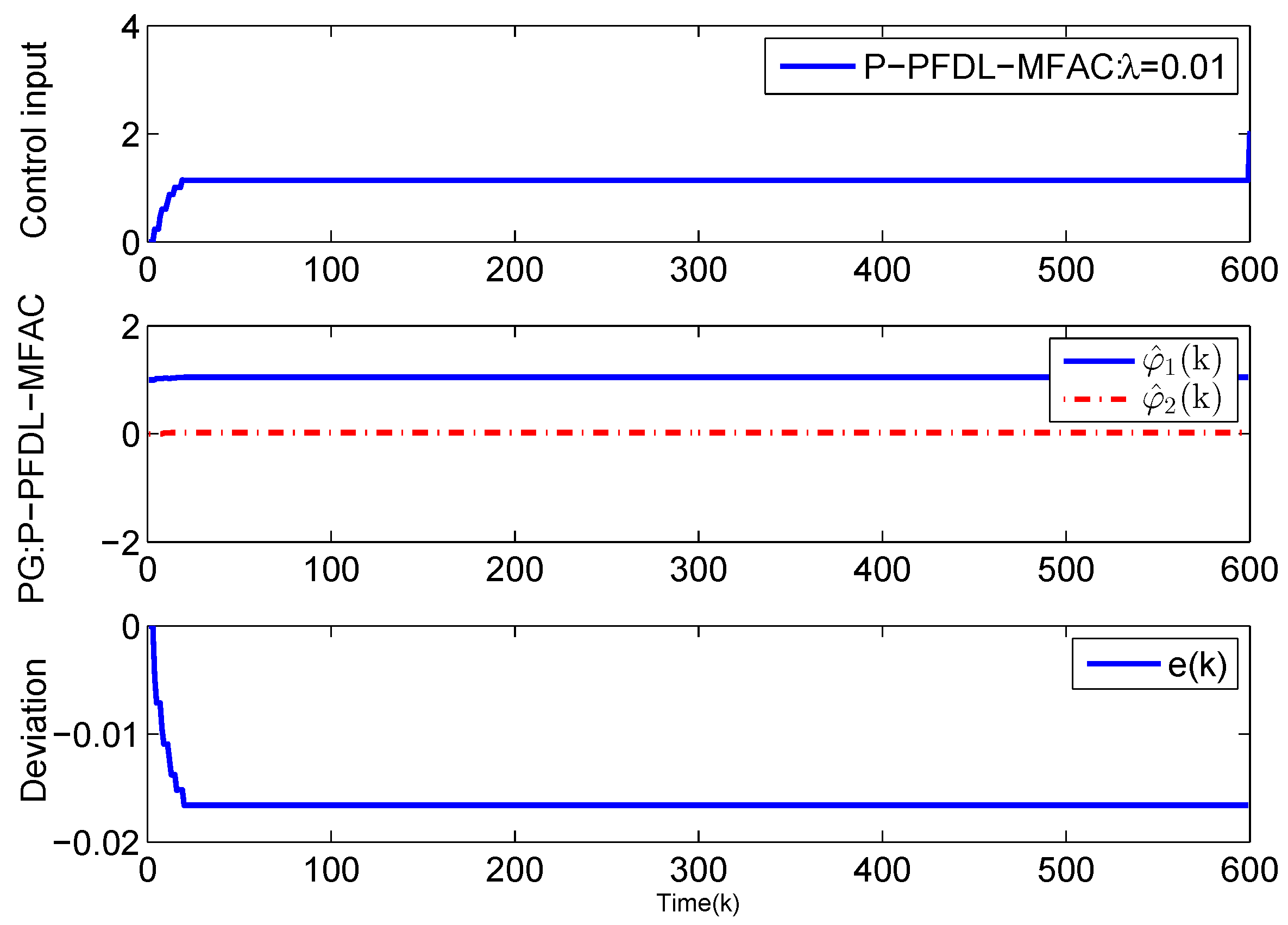
Set the initial conditions as , , , , , , . The controller parameters are set as , , , , , and the resetting initial value is . Figure 2 shows the system output process, and Figure 3 shows the curves of control input, PG estimation values, and deviation. From the controlled output of the system, it can be seen that although it has undergone drastic adjustment at the beginning, it can track the target quickly and achieve a good tracking effect.
Example 2.
A single input and three outputs of the nonlinear discrete-time system are given as follows.
where denotes one of the three outputs, ; is the Gaussian white noise and ; denotes the system input and ; the system is merely employed to produce the I/O data with unknown system structure, orders, and parameters.
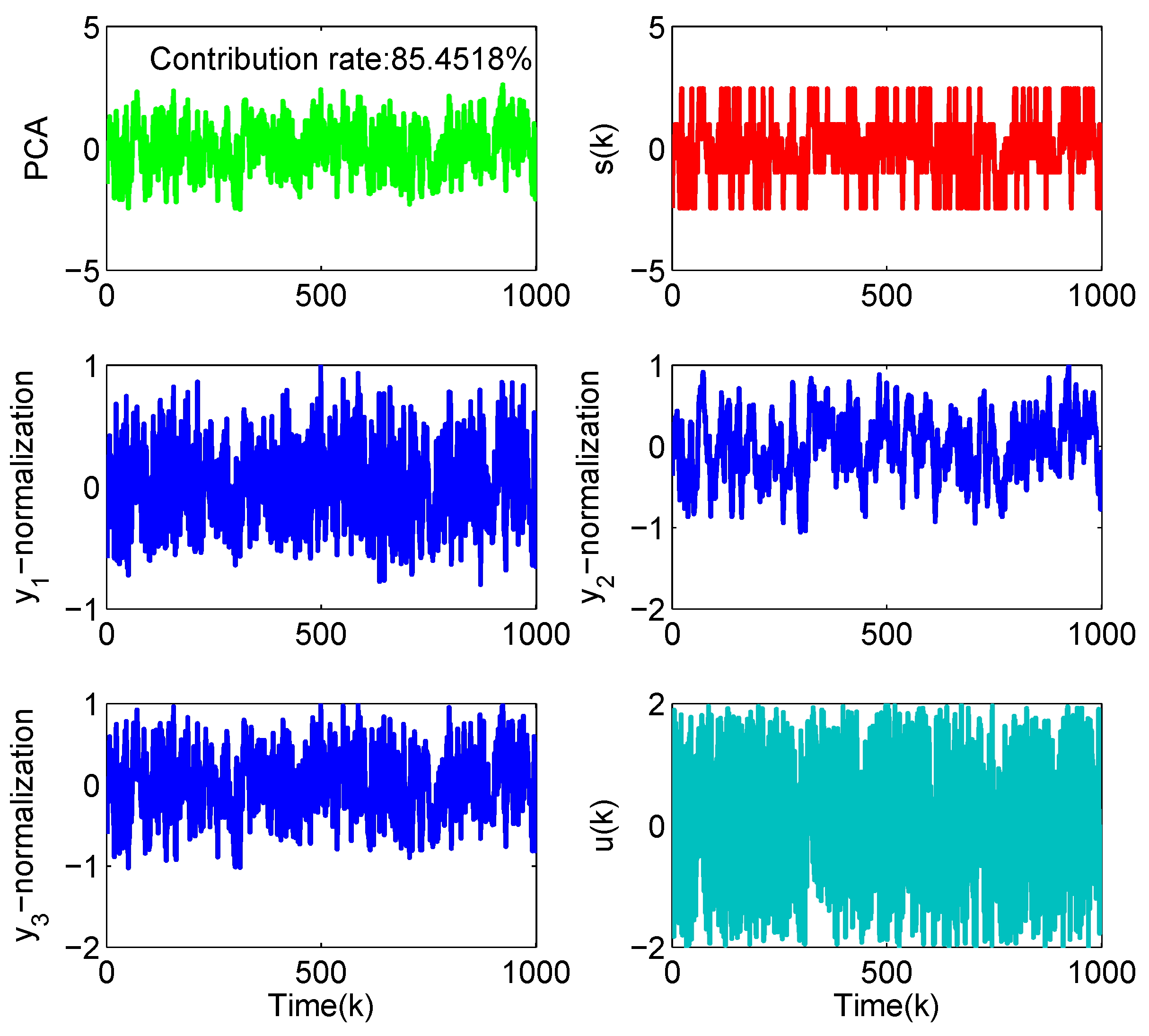
Feature extraction (), classification (), and metrics () of massive offline data. Here, 1000 evenly distributed inputs are taken and the corresponding outputs are obtained. The outputs are normalized and the PCA technology is employed to deal with them. One can obtain the first principal component information (the contribution rate: ). The same classification-metrics method (37) as in Example 1 is adopted. The parameter settings of the adopted classification method are , , . The distribution curves of , , , and are shown in Figure 4, . Table 2 shows the property values of each pattern class.
A pattern-moving-based system dynamics description is established as follows.
Nine pattern classes are obtained and the designed P-PFDL-PMFAC scheme (10)–(14) is employed to track the following targets.
where , denote that the object is pattern class 5 and 8, respectively.
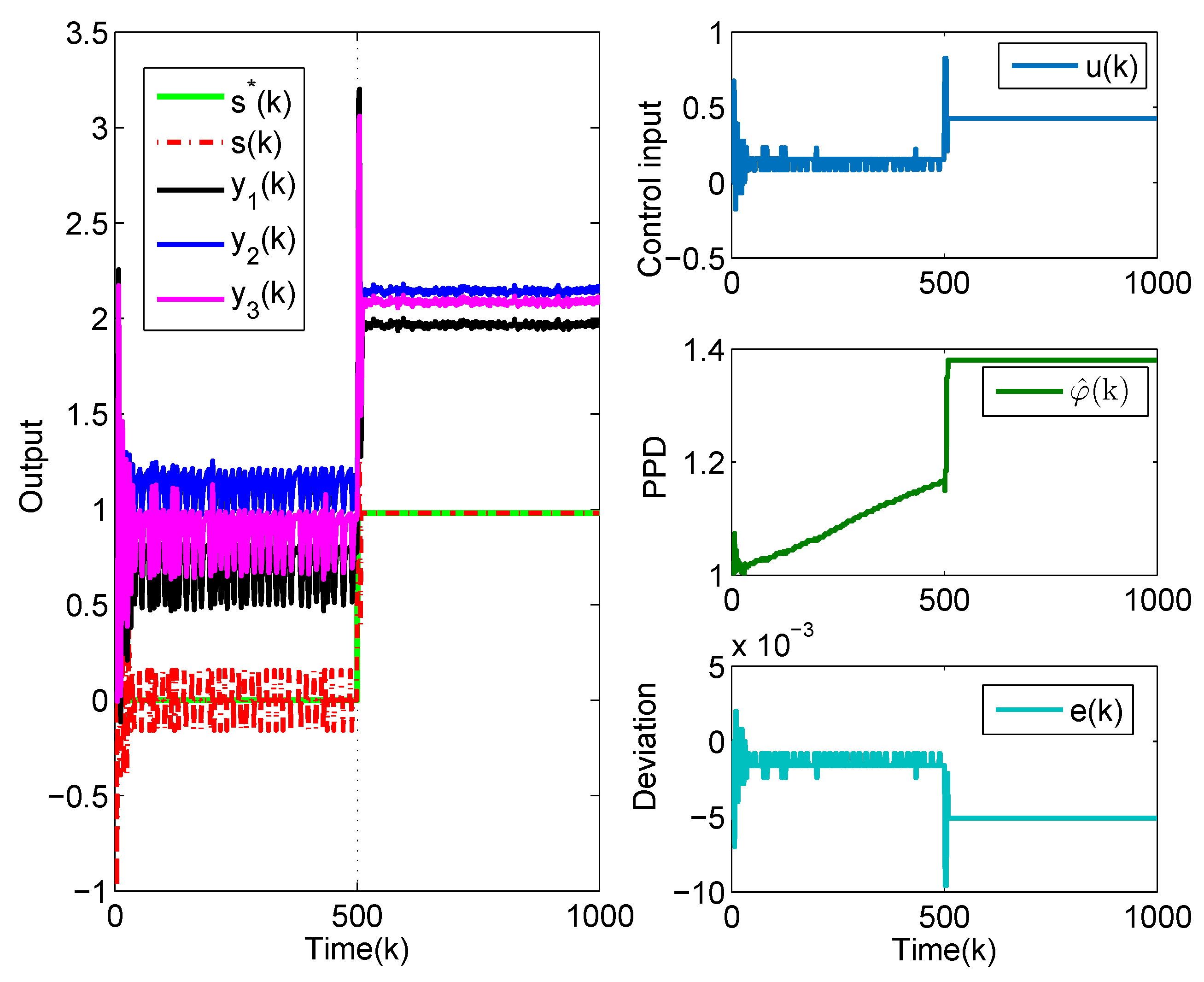
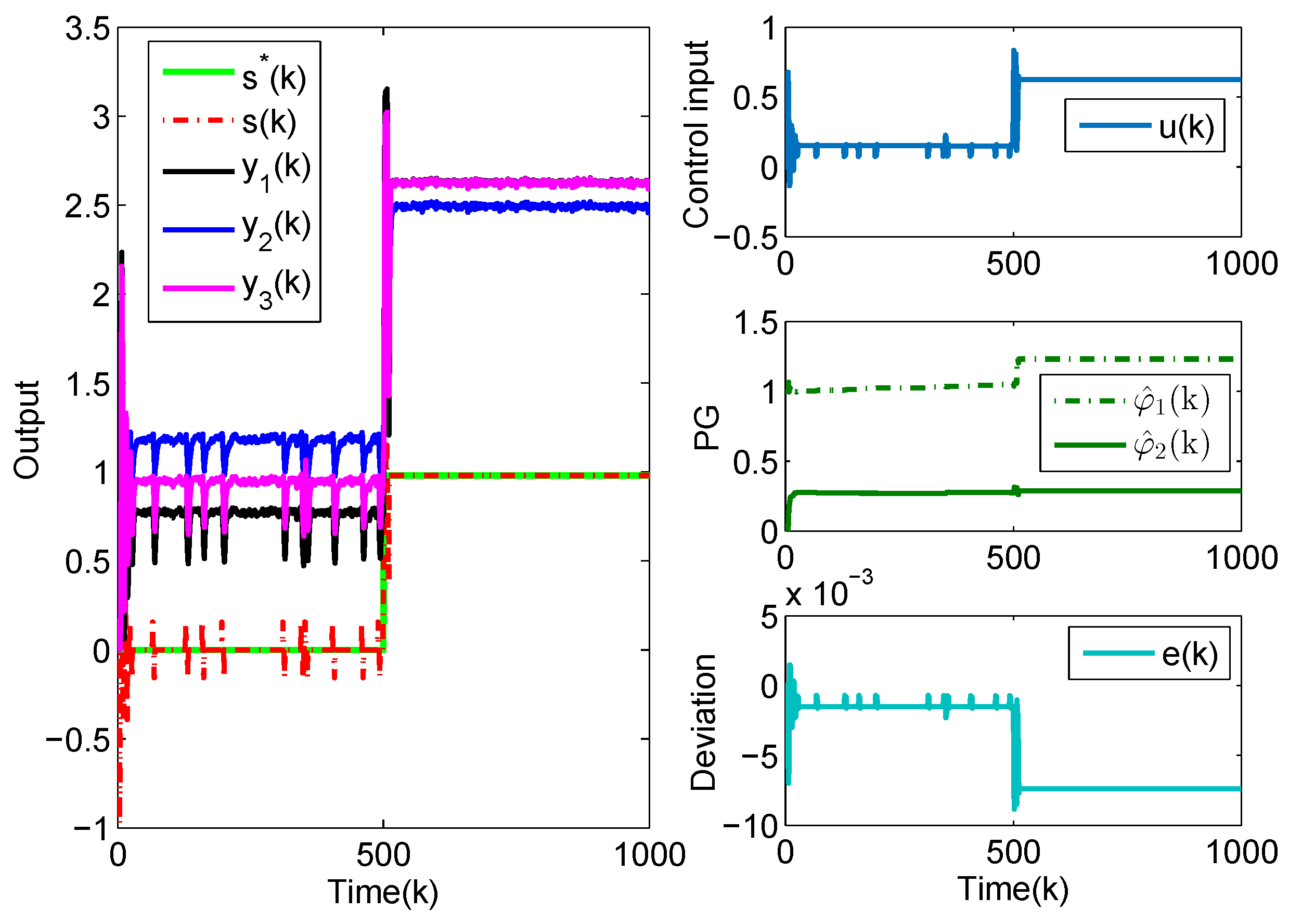
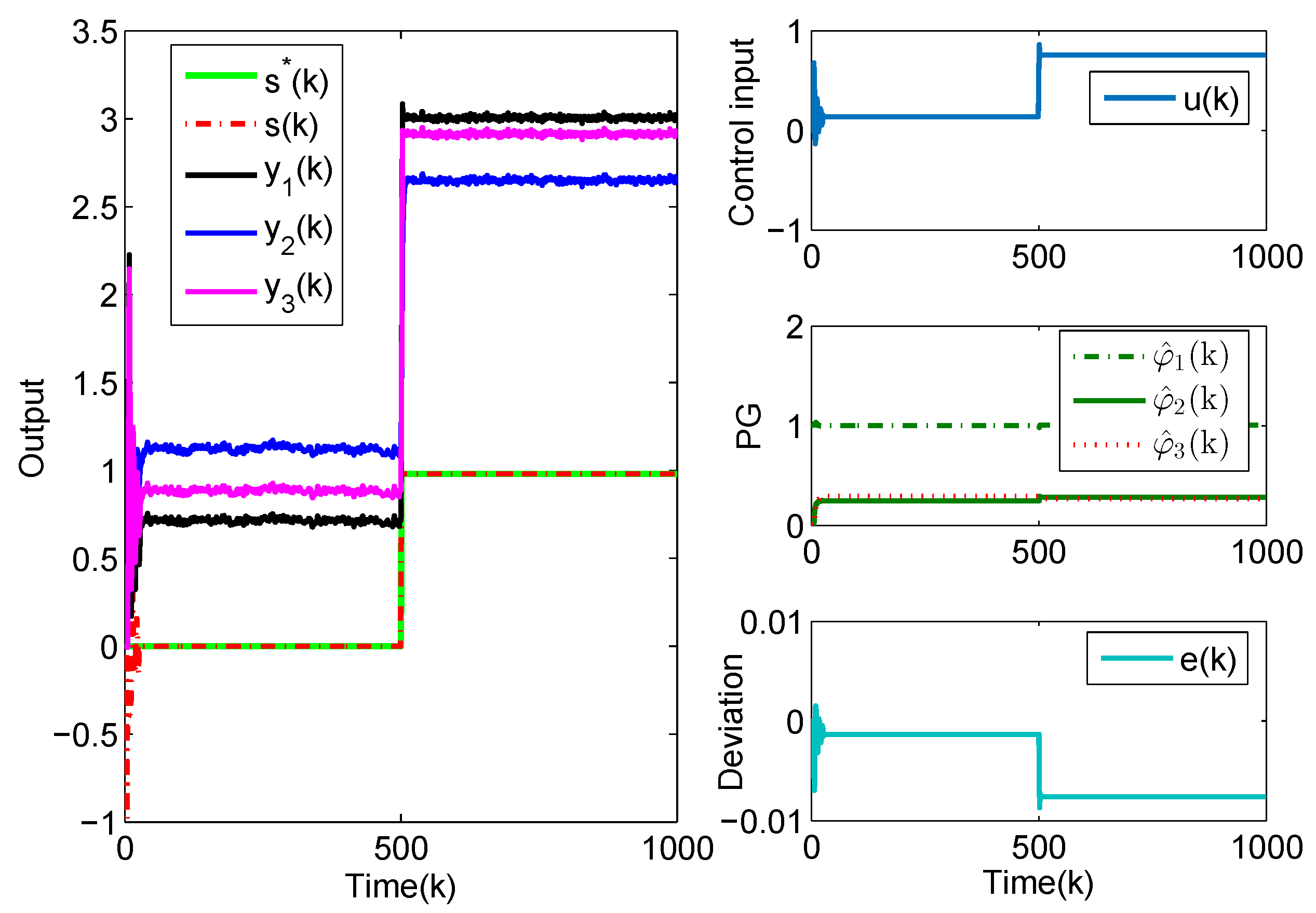
Set the initial conditions as , , , , , , , , , . The controller parameters are set as , , , , and the resetting initial value is . Figure 5, Figure 6 and Figure 7 correspond to the curves of system input, outputs, PG estimation values, and deviation when the pseudo-order l is 1, 2, and 3, respectively. When , the P-PFDL-PMFAC scheme degenerates to the P-CFDL-MFAC method designed in [30], and the PG vector becomes a PPD. All three figures show that the target trajectory is well tracked. However, Figure 5 shows that the tracking effect of target trajectory is poor. Figure 6 shows that the tracking effect of target trajectory is slightly better, but there are also many cases where the tracking can not be achieved. It can be seen from Figure 7 that the target object is well tracked. The simulation results confirm that the value of pseudo-order should correspond to the complexity of the system, and they show that a reasonable pseudo-order can improve the control effect of the system. This numerical example illustrates that the designed scheme is a very feasible method for a class of nonlinear discrete-time systems when the outputs only need to be controlled to one or some specific pattern classes.
6. Conclusions
A novel P-PFDL-MFAC scheme is proposed by combining the pattern-moving-based system dynamics description with the traditional PFDL-MFAC approach for a class of unknown practical SIMO nonaffine nonlinear discrete-time systems. Obviously, this scheme can also be applied to nonlinear or linear time-varying SISO systems, as long as the purpose of system control is to make all outputs belong to one or some pattern classes. Due to the existence of classification-metric deviation, an improved cost function for a deviation estimation algorithm and an adaptive tracking control law is designed based on the saddle point theory of TP-ZSG. The bounded convergence of the closed-loop system’s tracking error has been proven and the effectiveness of the P-PFDL-MFAC scheme has been validated via two simulation examples.
Although it can be seen from the simulation results that the control strategy proposed in this work has a good effect on the output disturbance, the robustness of data-driven control should also include the ability to deal with data dropout, which may be caused by sensor fault, transmission network failure, or actuator damage. Therefore, the next topic that needs to be focused on is the robustness of pattern-moving-based model free adaptive control in the case of missing data.
Author Contributions
Conceptualization, X.L. and Z.X.; methodology, Z.X.; software, X.L.; validation, X.L.; formal analysis, X.L.; investigation, X.L.; resources, X.L.; data curation, Z.X.; writing—original draft preparation, X.L.; writing—review and editing, X.L.; visualization, X.L.; supervision, Z.X.; project administration, X.L.; funding acquisition, X.L. All authors have read and agreed to the published version of the manuscript.
Funding
This study was supported by the National Natural Science Foundation of China (62076025).
Institutional Review Board Statement
Not applicable.
Informed Consent Statement
Not applicable.
Data Availability Statement
Not applicable.
Conflicts of Interest
The authors declare no conflict of interest.
References
- Yin, S.; Gao, H.; Kaynak, O. Data-driven control and process monitoring for industrial applications-Part I. IEEE Trans. Ind. Electron. 2014, 61, 6356–6359. [Google Scholar] [CrossRef]
- Qu, S.D. Pattern recognition approach to intelligent automation for complex industrial processes. J. Univ. Sci. Technol. Beijing 1998, 20, 385–389. [Google Scholar]
- Saridis, G.N. Application of pattern recognition method to control systems. IEEE Trans. Autom. Control 1981, 26, 638–645. [Google Scholar] [CrossRef]
- Zhu, Q.; Onori, S.; Prucka, R. Pattern recognition technique based active set QP strategy applied to MPC for a driving cycle test. In Proceedings of the 2015 American Control Conference, Chicago, IL, USA, 1–3 July 2015. [Google Scholar]
- Yu, B.; Zhang, X.; Wu, L.; Chen, X. A novel postprocessing method for robust myoelectric pattern-recognition control through movement pattern transition detection. IEEE Trans. Hum.-Mach. Syst. 2020, 50, 32–41. [Google Scholar] [CrossRef]
- Xu, Z. Pattern Recognition Method of Intelligent Automation and Its Implementation in Engineering. Doctoral Dissertation, University of Science and Technology Beijing, Beijing, China, 2001. [Google Scholar]
- Wang, M.; Xu, Z.; Guo, L. Stability and stabilization for a class of complex production processes via LMIs. Optim. Control Appl. Methods 2019, 40, 460–478. [Google Scholar] [CrossRef]
- Sun, C.; Xu, Z. Multi-dimensional moving pattern prediction based on multi-dimensional interval T-S fuzzy model. Control Decis. 2016, 31, 1569–1576. [Google Scholar]
- Guo, L.; Xu, Z.; Wang, Y. Dynamic modeling and optimal control for complex systems with statistical trajectory. Discret. Dyn. Nat. Soc. 2015, 2015, 1–8. [Google Scholar] [CrossRef]
- Tayebi-Haghighi, S.; Piltan, F.; Kim, J.M. Robust composite high-order super-twisting sliding mode control of robot manipulators. Robotics 2018, 7, 13. [Google Scholar] [CrossRef] [Green Version]
- Mobayen, S.; Tchier, F. A novel robust adaptive second-order sliding mode tracking control technique for uncertain dynamical systems with matched and unmatched disturbances. Int. J. Control Autom. Syst. 2017, 15, 1097–1106. [Google Scholar] [CrossRef]
- Yeh, Y.L. A Robust Noise-Free Linear Control Design for Robot Manipulator with Uncertain System Parameters. Actuators 2021, 10, 121. [Google Scholar] [CrossRef]
- Xi, X.; Mobayen, S.; Ren, H.; Jafari, S. Robust finitetime synchronization of a class of chaotic systems via adaptive global sliding mode control. J. Vib. Control 2018, 124, 3842–3854. [Google Scholar] [CrossRef]
- Skruch, P. A terminal sliding mode control of disturbed nonlinear second-order dynamical systems. J. Comput. Nonlinear Dyn. 2016, 11, 054501. [Google Scholar] [CrossRef]
- Xu, Z.; Wu, J.; Guo, L. Modeling and optimal control based on moving pattern. In Proceedings of the 32nd Chinese Control Conference, Xi’an, China, 26–28 July 2013. [Google Scholar]
- Xu, Z.; Wu, J. Data-driven pattern moving and generalized predictive control. In Proceedings of the 2012 IEEE International Conference on Systems, Man and Cybernetics, Seoul, Korea, 14–17 October 2012. [Google Scholar]
- Hou, Z.S.; Xiong, S.S. On model-free adaptive control and its stability analysis. IEEE Trans. Autom. Control 2019, 11, 4555–4569. [Google Scholar] [CrossRef]
- Gao, W.; Jiang, Y.; Jiang, Z.; Chai, T. Output-feedback adaptive optimal control of interconnected systems based on robust adaptive dynamic programming. Automatica 2016, 72, 37–45. [Google Scholar] [CrossRef] [Green Version]
- Ahn, H.; Chen, Y.; Moore, K. Iterative learning control: Brief survey and categorization. IEEE Trans. Syst. Man. Cybern. Part C Appl. Rev. 2007, 37, 1099–1121. [Google Scholar] [CrossRef]
- Hjalmarsson, H.; Gevers, M.; Gunnarsson, S.; Lequin, O. Iterative feedback tuning: Theory and applications. IEEE Control Syst. Mag. 1998, 18, 26–41. [Google Scholar]
- Campi, M.C.; Lecchini, A.; Savaresi, S.M. Virtual reference feedback tuning: A direct method for the design of feedback controllers. Automatica 2002, 38, 1337–1346. [Google Scholar] [CrossRef] [Green Version]
- Hou, Z.S.; Jin, S.T. A novel data-driven control approach for a class of discrete-time nonlinear systems. IEEE Trans. Control Syst. Technol. 2011, 19, 1549–1558. [Google Scholar] [CrossRef]
- Hou, Z.S.; Jin, S.T. Model Free Adaptive Control: Theory and Applications; CRC Press: Boca Raton, FL, USA, 2013. [Google Scholar]
- Hou, Z.S.; Liu, S.D.; Tian, T.T. Lazy-learning-based data-driven model-free adaptive predictive control for a class of discrete-time nonlinear systems. IEEE Trans. Neural Netw. Learn. Syst. 2017, 28, 1914–1928. [Google Scholar] [CrossRef] [PubMed]
- Wang, Z.S.; Liu, L.; Zhang, H.G. Neural network-based model-free adaptive fault-tolerant control for discrete-time nonlinear systems with sensor fault. IEEE Trans. Syst. Man Cybernet Syst. 2017, 47, 2351–2362. [Google Scholar] [CrossRef]
- Li, H.T.; Ning, X.; Li, W.Z. Implementation of a MFAC based position sensorless drive for high speed BLDC motors with nonideal back EMF. ISA Trans. 2017, 67, 348–355. [Google Scholar] [CrossRef] [PubMed]
- Bu, X.H.; Hou, Z.S.; Zhang, H.W. Data driven multiagent systems consensus tracking using model free adaptive control. IEEE Trans. Neural Netw. Learn. Syst. 2018, 29, 1514–1524. [Google Scholar] [CrossRef] [PubMed]
- Treesatayapun, C. Varying-sliding condition adaptive controller for a class of unknown discrete-time systems with data-driven model. Int. J. Model. Identif. Control 2017, 27, 210–218. [Google Scholar] [CrossRef]
- Zhu, Y.M.; Hou, Z.S.; Qian, F.; Du, W.L. Dual RBFNNs based model free adaptive control with aspen HYSYS simulation. IEEE Trans. Neural Netw. Learn. Syst. 2017, 28, 759–765. [Google Scholar] [CrossRef]
- Li, X.Q.; Xu, Z.G.; Lu, Y.L.; Cui, J.R.; Zhang, L.X. Modified Model Free Adaptive Control for a Class of Nonlinear Systems with Multi-threshold Quantized Observations. Int. J. Control. Autom. Syst. 2021. [Google Scholar] [CrossRef]
- Sun, J.L.; Liu, C.S. Distributed zero-sum differential game for multi-agent systems in strict-feedback form with input saturation and output constraint. Neural Netw. 2018, 106, 8–19. [Google Scholar] [CrossRef]
- Song, R.Z.; Zhu, L. Stable value iteration for twoplayer zero-sum game of discrete-time nonlinear systems based on adaptive dynamic programming. Neurocomputing 2019, 340, 180–195. [Google Scholar] [CrossRef]
- Yang, J.; Zhang, D.; Frangi, A.F.; Yang, J. Two- dimensional PCA: A new approach to appearance-based face representation and recognition. IEEE Trans. Pattern Anal. Mach. Intell. 2008, 26, 131–137. [Google Scholar] [CrossRef] [Green Version]
- Guo, G.J.; Chen, T.W. A new approach to quantized feedback control systems. Automatica 2008, 44, 534–542. [Google Scholar] [CrossRef]
- Bu, X.H.; Qiao, Y.X.; Hou, Z.S.; Yang, J.Q. Model free adaptive control for a class of nonlinear systems using quantized informtion. Asian J. Control 2018, 20, 962–968. [Google Scholar] [CrossRef]
- Bu, X.H.; Zhu, P.P.; Yu, Q.X.; Hou, Z.S.; Liang, J.Q. Model-free adaptive control for a class of nonlinear systems with uniform quantizer. Int. J. Robust Nonlinear Control 2020, 30, 6383–6398. [Google Scholar] [CrossRef]
- Li, X.L.; Wang, S.N. Application of multimodel adaptive control algorithm in robotic manipulator control. Robot 2002, 24, 16–19. [Google Scholar]
- Koivo, A.; Guo, T. Adaptive linear controller for robotic manipulators. IEEE Trans. Autom. Control 1983, 28, 162–171. [Google Scholar] [CrossRef]
Figure 1.
The curves of I/O data and class centers.

Figure 2.
The curves of desired class center, original output, and its corresponding class center.

Figure 3.
The curves of control input, PG estimation values, and deviation.

Figure 4.
The curves of I/O data, PCA information, and class center.

Figure 5.
The curves of PPD estimation value, control input, deviation, and outputs with .

Figure 6.
The curves of PG estimation values, control input, deviation, and outputs with .

Figure 7.
The curves of PG estimation values, control input, deviation, and outputs with .


Table 1.
Property values of pattern class.
| Class No. | Class Center | Class Radius | Threshold |
|---|---|---|---|
| 1 | |||
| 2 | |||
| 3 | |||
| 4 | |||
| 5 | |||
| 6 | |||
| 7 | |||
| 8 | |||
| 9 | |||
| 10 | |||
| 11 |
Table 2.
Property values of pattern class.
| Class No. | Class Center | Class Radius | Threshold |
|---|---|---|---|
| 1 | |||
| 2 | |||
| 3 | |||
| 4 | |||
| 5 | |||
| 6 | |||
| 7 | |||
| 8 | |||
| 9 |
Publisher’s Note: MDPI stays neutral with regard to jurisdictional claims in published maps and institutional affiliations. |
© 2021 by the authors. Licensee MDPI, Basel, Switzerland. This article is an open access article distributed under the terms and conditions of the Creative Commons Attribution (CC BY) license (https://creativecommons.org/licenses/by/4.0/).
Share and Cite
MDPI and ACS Style
Li, X.; Xu, Z. Pattern-Moving-Based Partial Form Dynamic Linearization Model Free Adaptive Control for a Class of Nonlinear Systems. Actuators 2021, 10, 223. https://0-doi-org.brum.beds.ac.uk/10.3390/act10090223
AMA Style
Li X, Xu Z. Pattern-Moving-Based Partial Form Dynamic Linearization Model Free Adaptive Control for a Class of Nonlinear Systems. Actuators. 2021; 10(9):223. https://0-doi-org.brum.beds.ac.uk/10.3390/act10090223
Chicago/Turabian StyleLi, Xiangquan, and Zhengguang Xu. 2021. "Pattern-Moving-Based Partial Form Dynamic Linearization Model Free Adaptive Control for a Class of Nonlinear Systems" Actuators 10, no. 9: 223. https://0-doi-org.brum.beds.ac.uk/10.3390/act10090223
Note that from the first issue of 2016, this journal uses article numbers instead of page numbers. See further details here.