
Probability Methods for Stability Design of Open Pit Rock Slopes: An Overview


1
Department of Mining & Metallurgical Engineering, Western Australian School of Mines (WASM), Curtin University, Bentley, WA 6102, Australia
2
Key Laboratory of Ministry of Education for Safe Mining of Deep Metal Mines, Northeastern University, Shenyang 110819, China
*
Authors to whom correspondence should be addressed.
Geosciences 2021, 11(8), 319; https://0-doi-org.brum.beds.ac.uk/10.3390/geosciences11080319
Submission received: 23 February 2021
/
Revised: 13 July 2021
/
Accepted: 22 July 2021
/
Published: 28 July 2021
(This article belongs to the Special Issue Rockfall Hazard)
Abstract
:The rock slope stability analysis can be performed using deterministic and probabilistic approaches. The deterministic analysis based on the safety concept factor uses fixed representative values for each input parameter involved without considering the variability and uncertainty of the rock mass properties. Probabilistic analysis with the calculation of probability of failure instead of the factor of safety against failure is emerging in practice. Such analyses offer a more rational approach to quantify risk by incorporating uncertainty in the input variables and evaluating the probability of the failure of a system. In rock slope engineering, uncertainty and variability involve a large scatter of geo-structural data and varied geomechanical test results. There has been extensive reliability analysis of rock slope stability in the literature, and different methods of reliability are being employed for assessment of the probability of failure and the reliability of a slope. Probabilistic approaches include Monte Carlo simulation (MCS), the point estimate method (PEM), the response surface method (RSM), first- and second-order reliability methods (FORMs and SORMs), and the first-order second-moment method (FOSM). Although these methods may be complicated, they provide a more complete definition of risk. Probabilistic slope stability analysis is an option in most commercial software; however, the use of this method is not common in practice. This paper provides an overview of the literature on some of the main probabilistic reliability-based methods available for the design of the rock slope in open pit mining. To demonstrate its applicability, the paper investigates the stability of a rock slope in an open pit mine in the Goldfields region, Western Australia. Two different approaches were adopted: deterministic stability analysis using two-dimensional limit equilibrium and finite element shear strength reduction methods using SLIDE and RS2 software, respectively, and probabilistic analysis by applying the MCS and RSM methods in the limit equilibrium method. In this example, the slope stability analysis was performed using the Spencer method with Cuckoo search optimization to locate the critical slip surface. The results obtained were compared and commented on.
1. Introduction
Probability analysis of rock slopes has gained considerable attention in the design of open pit mines (e.g., [1,2,3,4,5,6]). The unavoidable uncertainties involved in geotechnical design parameters has, however, attracted significant research in the use of reliability analysis of slope stability over the past few decades [7,8,9,10,11,12]. In most cases, the stability of the open pit slope is expressed in terms of the factor of safety. The factor of safety is determined by the deterministic methods, which include limit equilibrium (LEM) and the shear strength reduction method (SSRM). For complex cases of variable slope geometry and geological settings, deterministic methods cannot be applied. The natural variability in rock properties is the direct result of various factors that the rocks are subjected to during their formation [13]. The complexity comes from the variabilities and uncertainties associated with the rock properties during the design and assessment of rock slope stability. This natural variability cannot be reduced no matter our knowledge of rock properties and expertise displayed in estimating them [13,14]. On the other hand, knowledge-based uncertainties can be reduced, if not eliminated. Unlike the natural variability, the magnitude of knowledge-based uncertainties reduces as the level of knowledge increases [13,14]. Therefore, in the deterministic approach, the factor of safety cannot reflect the uncertainty of its underlying parameters. In most cases, the influence of a parameter on the calculated factor of safety is investigated through a sensitivity analysis, based on the recognition that there are many uncertainties associated with the underlying parameters [15,16].
Therefore, the most appropriate approach is to consider the stability analysis as a random system where the occurrence of slope failure is a random event and analyze it with the probability method. The use of probability methods in slope engineering permits a rational treatment of the various uncertainties that significantly influence the safety of a rock slope. These methods assume that the input parameters are of a random character that depends not only on the mean values of the parameters but also on their scatter and correlation. In other words, the probability methods allow a systematic approach of treating uncertainties and quantifying the reliability of a design [11,12,14,15,16,17,18,19,20,21]. In a probability analysis, every input parameter is assigned a statistical distribution, and stability is evaluated in terms of the probability of failure (Pf) and/or reliability index (β); Pf is the probability that the factor of safety is less than unity or a reference value. As an example, the relationship between β and Pf is presented in Table 1 [22]. Geotechnical designs typically require a β > 3.0 (i.e., Pf = 0.001) for an expected performance better than “above average”.
Both LEM and SSRM, although originally deterministic, can easily be adapted to suit probabilistic models [23]. The probability of failure and the reliability index are used to quantify risks and hence evaluate the consequence of failure [24]. Various probability methods have been proposed to estimate Pf and/or β (e.g., [14,25,26,27,28]). The most widely used methods are the first-order reliability method (FORM) (e.g., [29,30,31]), first-order second-moment (FOSM) method (e.g., [7,26]), and second-order reliability method (SORM) (e.g., [32,33]). The reliability-based design approach has been developed and utilized to address the shortcomings of the deterministic approach and considers uncertainties explicitly [14,34]. Several applications of solution methods using Monte Carlo simulation (e.g., [35,36,37]), the point estimate method (e.g., [19,38,39]), and the response surface method (RSM) have been reported in the literature (e.g., [32,40,41]). [7] explored the mean first-order reliability method, which is a simplification of the more general first-order reliability method. [21] used FORM to model rock plane failure. [42] used Monte Carlo simulation as sensitivity tool for calculating the probability of failure [43]. The reliability methods and the response surface methods have been used for slope reliability problems with an implicit performance function (e.g., [40]).
The early applications of reliability methods (e.g., [44,45,46,47,48]) were limited to theoretical case studies. Currently, the probability and reliability methods for slope stability constitute an already well-developed research area and most of the methods are currently implemented in numerical code for the design of rock slopes in practice. The most important literature in this area includes journal articles and books (e.g., [14,49,50,51]). Although the system reliability methods have been used extensively in theoretical cases and in civil engineering applications, these approximation methods may not be available for practical open pit slopes with complicated geometry and/or multiple slope bench due to the perceived mathematical complexity. More importantly, with the advent of computers in data handling, Monte Carlo simulation, Latin hypercube, and the response surface method (RSM) have been adopted in LEM software programs, such as SLIDE. The SSRM methods, however, have been adopted in several well-known finite element (RS2/3) or finite difference (FLAC) programs. In addition, the FOSM, for instance, is time consuming, which is quite common for the implicit performance for LEM analysis [52]; however, researchers have tried to overcome these problems using methods like RSM [53]. Recently, [53] used Gaussian process regression (GPR) and genetic programming (GP) to resolve the problems of the implicit function performance function. This GPR is a nonparametric kernel-based probabilistic model.
However, while LEM is the most widely used method for evaluating slope stability in practice, extensive research has been undertaken to improve its performance, particularly in finding the global critical slip surface [23]. Again, while the determination of the critical slip surface may be affected by the experience of the researcher or engineer, several search algorithms, such as the cuckoo, particle swam optimization, simulated annealing, etc., have been proposed to optimize the search for the critical slip surface. On the other hand, to carry out a probabilistic analysis using SRM, a spatially correlated field is typically developed in random field theory and then solved using finite element or finite difference methods [54].
This paper aims to review some probability methods that have been used in the design of rock slope reliability problems. A brief discussion of the uncertainty and variability associated with rock mass and some methods of quantification is presented. Then, the cuckoo and particle swam optimization search methods are briefly discussed. Based on existing knowledge of the uncertainty associated with rock slopes, and the limitation of the implicit reliability functions, the paper adopts the cuckoo techniques coded in the Rocscience SLIDE computer software to analyze the stability of a case pit slope located in the Goldfields, Western Australia. Deterministic and probabilistic analyses were carried out using LEM using the Rocscience SLIDE computer software to determine the factor of safety, probability of failure, and reliability index. The reliability of the case pit slope stability was evaluated using Monte Carlo simulation and the response surface method and the results were compared.
2. Uncertainty in Rock Slope Engineering and Methods of Quantification
In general, sources of uncertainty in slope engineering include the natural variability of the rock material, limited availability of information about the ground condition, and errors made during measurements and testing of samples [55]. There are various classifications of uncertainty in the literature; however, one classification that proves adequate for geotechnical engineers places uncertainty into three groups (Figure 1): geological uncertainty, model uncertainty, and parameter uncertainty [14,56,57]. Geological uncertainty comprises uncertainties associated with the geometry of geological structures and their relationships between lithologies and those associated with the boundaries of lithologies [56,58]. Model uncertainty exists if there is a possibility of obtaining an incorrect result even if the exact values are available for all the model parameters [56]. It reflects the inability of a model or design technique to represent the true physical behavior of a system under consideration [14,58,59]. Parameter uncertainty reflects the inability to account for the various attributes of the geotechnical model [56]. It includes uncertainties associated with the values adopted for the rock mass and hydrogeological model parameters, which can stem from data scatter, such as the spatial variability and random testing error and systematic error, which involves statistical error and bias in measurements.
As uncertainty is present in the in situ material, it means uncertainty will also exist in the expected performance function of the design [60]. If a value of the performance function like cohesion or the friction angle varies, and this variation over space and time cannot be predicted, one cannot say with certainty what the value of the variable will be but only the likelihood or probability that it will be within some specific range of values. Unfortunately, the overall uncertainty is rarely quantified in rock engineering. Instead, conservative designs are generally adopted through deterministic analysis. However, as single values are assigned in the deterministic analyses, there is no guarantee that the design will perform as expected. Therefore, there is the need to have an approach that can consider varying rock variabilities and uncertainties in rock slope conditions during the design of rock slopes and analysis of rock slope stability.
Various mathematical frameworks have been developed for the assessment of uncertainty and variability in slope stability analysis (e.g., [7,8,11,12,14,19,25,32,34,35,37,55,61,62,63,64,65]). Two main methodologies have been proposed to deal with uncertainties in the rock properties in the assessment of slope stability, i.e., the reliability method and non-deterministic methods [66]. As shown in Figure 2, the non-deterministic methods consist of probabilistic methods and non-probabilistic methods (also called imprecise methods). In the probabilistic methods, the rock properties affecting the stability of the slope are considered as random variables that have a certain probability distribution. Some of the common non-probabilistic methods are evidence theory, fuzzy set theory, the interval approach, possibility theory, random set theory, etc. [58,66]. For instance, uncertainty characterized by fuzziness is treated with a branch of methodologies based on a fuzzy representation of uncertain variables. A complete description of each method is outside the scope of this paper and the reader is referred to the documents cited for more information on the mathematical formulations and procedures. A brief description of FORM, FOSM, SORM, PEM, MCS, and RSM is given in the next section to provide some insight on the mathematical meaning. Reliability analyses provide a more rational approach to quantity slope design risk than a deterministic method by incorporating uncertainty in the input parameters in the analysis. By doing so, the probability of failure can be established for a specific failure mode.
3. Review of Reliability-Based Methods
3.1. Reliability Index and Probability of Failure
The main task of reliability analysis is to calculate the probability of failure and reliability index. To perform a reliability analysis, a performance function g(X) must be defined that relates to the resistance R(X) and disturbance S(X) acting on the system. This is mathematically expressed as:
where X represents the collection of random input variables. By this definition, failure occurs if g(X) < 0, while g(X) > 0 denotes stable conditions (Figure 3). The surface defined by g(X) = 0 is referred to as the critical limit state as it defines the boundary between these two conditions [60]. When considering the critical limit state for a rock slope under planar failure, the performance function can be expressed as the shear strength that resists sliding minus the shear forces that initiate sliding. Such equations can be evaluated analytically with little additional effort. For more complex problems, such as an analysis of rock slope deformation under seismic conditions, it is difficult to define the loads and resistances explicitly. Approximate methods of evaluation are therefore required.
g(X) = R(X) − S(X)
To calculate the reliability of the system, the distance between the mean value of the performance function and the critical limit state at g(X) = 0 must be determined. When the distance between these two points is normalized with respect to the standard deviation of the performance function, this is referred to as the reliability index β for the system (Figure 3). The reliability index is defined as [60]:
where μg and σg are the mean and standard deviation of the performance function, respectively. However, to solve for the value of β in Equation (2), the exact shape of the performance function must be known, which is not always the case. Based on this, a more versatile measurement of reliability is the Hasofer–Lind reliability index βHL. This method, also known as the first-order reliability method (FORM), calculates the minimum distance in units of the directional standard deviation from the mean value point of the multivariate distribution of the random variables to the boundary of the critical limit state (Figure 3). This provides a more consistent and invariant measure of reliability for the system and can also be easily calculated for correlated or uncorrelated variables using the approach outlined in [29]. The matrix equation for βHL can be defined as [60]:
or:
where X is the vector of random variables of the set random variable, μ is the vector of mean values of random variables, σ is the standard deviation, and F defines the failure region of g(X) < 0. The variable C defines the covariance matrix and R is the correlation matrix, which allows the user to establish either a positive or negative relationship between random variables. Equation (4) is preferred to Equation (3) because the correlation matric R is easier to set up and conveys the correlation structure more explicitly than the covariance matrix. For uncorrelated variables, the matrix R simplifies to a symmetric unit matrix. The matrix algebra may be unfamiliar to some; however, programs, such as Microsoft Excel or MATLAB, can be used to easily complete these calculations (e.g., [29,31,67]).
After the reliability index has been determined, the probability of failure Pf for the system can be found by calculating the probability of g(X) < 0 (Figure 3). This is related to the reliability index using the following equation:
where Φ is the cumulative distribution function (CDF) for the performance function evaluated at 0 with a unit standard deviation and a mean β. As mentioned earlier, the shape of the distribution is rarely known and therefore must be assumed. In most cases, a normal distribution is reasonable; however, a truncated or lognormal distribution may be more appropriate when the performance function depends on positive functions, such as the factor of safety, extent of yield in a material, or displacements [60].
Again, from Equation (2), a constant mean value suggests that the reliability index increases, and the uncertainty in the estimate of the performance function decreases. This results in a narrower distribution for the performance function and a decrease in the probability of failure for the system. FORM is widely used because of its efficiency. However significant errors may arise when the nonlinearity of the failure/performance function increases. This nonlinearity is due to the nonlinear relationship between random variables, the consideration of non-normal random variables, and/or the transformation from a correlated to uncorrelated random variable [24]. As many of the reliability methods are based on approximations, it is likely that different methods will produce different results. Different methods must be compared to obtain a more accurate understanding of a system. There are two variations of FORM, i.e., FOSM and AFOSM. In FOSM, the statistical distribution of the random variables is ignored whereas in AFOSM, the distribution of the random variables is considered.
3.2. Reliability Methods
As mentioned earlier, for a more a complex problem, the performance function cannot be stated explicitly. The reliability methods are normally coupled with the finite element method to evaluate the performance function. The number of evaluations and what input parameters are selected depend on the reliability methods used [60]. The following section briefly describes five methods that can be used to approximate the statistical moments of the performance function.
3.2.1. First Order Second Moment
FOSM has long been applied to assess the reliability of slopes [68]. It consists of the Taylor series of approximations of the mean and variance of the performance function. Where the performance function is smooth and regular, the mean and variance can be calculated using the first terms of the Taylor series expansion method to expand g(X) [69,70]. It requires a linearized form of the performance function at the mean values of the random variables [24,70]. This method assumes that the expected value of the performance function is approximately equal to the value of the function calculated with the mean values of all variables [60,70]. The variance is determined by calculating the partial derivatives of the performance function with respect to each uncertain variable. For uncorrelated input random variables, the variance of the function is given as:
where Xi denotes the random variables and n is the number of random variables. As stated earlier, since the performance function cannot be stated explicitly in most geotechnical engineering applications, a linear approximation for the partial derivatives is required [70]. To achieve this, each of the variables is changed by a small (ΔXi) amount while all other variables are kept at their mean values. The change in the performance (ΔG) that results is then divided by the difference in the input. Therefore, to maintain a consistent level of uncertainty, the input variables are chosen at the mean plus and minus one standard deviation, and Equation (6) can be revised as [60]:
3.2.2. Second-Order Reliability Method
SORM was initially studied by [71,72]. The method was developed to enhance the accuracy of the estimated probability of failure. Since the performance function is approximated by a linear function, the accuracy of FORM deteriorates when the nonlinearity of a limit state function increases. In other words, SORM overcomes the disadvantage of FORM. SORM is more computationally expensive than FORM since a second derivative is required. Once the second-order surface is obtained, according to the asymptotic formula of Breitung, the probability of failure can be calculated. Breitung’s formulation [72] for SORM is given by [73]:
where vi (i = 1, …, n − 1) are the principal curvatures of the limit state function at the most probable point (MPP) and β is the reliability index obtained from FORM. MPP is the point that has the highest probability density on the performance g(X) = 0 as shown in Figure 4. The principal curvatures of the limit state surface are obtained as the eigenvalues of the rotational transformed second-order derivatives matrix called the Hessian matrix of the performance function in the standard normal space [74]. In attempt to address this problem, a number of studies have been performed aiming to eliminate the calculation of the Hessian matrix (e.g., [73,75,76,77]). The other popular formulation is given by [78], which is considered more accurate than Breitungs’s formulation [73,76,77]. Ref [73] modified SORM, called the second-order reliability method with first-order efficiency (SORM-FOE). According to [73], if the derivatives of the MPP search are evaluated numerically, the number of functions required for FORM will be linearly proportional to the number of random variables n as [73,74]:
where k represents the number of iterations of the MPP search. However, if the finite difference formula is used for the derivative evaluation, the number of functions required by SORM is:
Clearly, the SORM is second-order efficient because NSORM is quadratic in terms of n. SORM-FOE improves the accuracy of FORM while maintaining a similar level of efficiency [73].
3.2.3. Point Estimate Method
The point estimate method (PEM) originally proposed by [79,80] is one of the most popular numerical procedures that approximates the expected value and the variance of a performance function by evaluating it as a series of specifically chosen discrete points. Evaluation of the points is chosen at the mean plus and mean minus one standard deviation for each variable, resulting in 2n evaluations for n random variables. A weighting value ρ is used at each evaluation point to ensure the expected (mean) value and standard deviation of the input parameters are recovered [19,39,59,60,81,82]. The method accounts for a maximum of three statistical moments, namely mean, variance or standard deviation, and skewness. It does not require prior knowledge of the shape of any probability density function of the input variables and the spatial correlation; however, this approximate method may lead to incorrect interpretations of the reliability if the var function g(X) is highly nonlinear or the random variables are asymmetric. According to [60], if all the evaluation points are weighted equally, this value is 1/n for each variable. The statistical mean and variance are given by the following equations:
where xi is the input variable, g(xi) is the function of the input variable xi, and n is the number of variables. When the coefficients of variation for the input parameters are small, PEM is found be robust; however, the number of evaluations can be significantly high when a large number of variables are considered. [83], including several other authors, have developed methods to reduce the number of evaluations, and users need to be mindful of the assumptions [60,81,82].
3.2.4. Monte Carlo Simulation
The Monte Carlo (MC) simulation method is considered a very powerful tool. It was developed in 1949 by John von Neumann and Stanislav Ulam when they published a paper “the Monte Carlo method”. Due to its robustness and concept simplicity, it has been widely used in reliability analyses [14,34,37,84,85]; it provides efficiency for engineers with basic working knowledge of probability and statistics for risk evaluation of risk or reliability of complex engineering systems. Thus, when the behavior of the performance function is difficult to evaluate, the probability of failure can be calculated directly by using Monte Carlo simulation. In this method, large sets of randomly selected input variables are generated according to their probability distribution function in the analytical model to determine the behavior of the system [60,82]. The method generates a random number for each of the input random variables in the problem and it makes combinations amongst all these random variables to perform several deterministic computations [5,86]. The accuracy of the method depends on the number of simulations performed and increases with an increasing number of simulations. Though the method has some advantages, it can be computationally intensive and time consuming. However, the lack of approximations makes Monte Carlo an ideal standard to compare to other reliability methods.
3.2.5. Response Surface Method
The response surface method (RSM) has been presented as an efficient tool to identify the likelihood of the failure behavior of rock slopes [87]. The method has been applied in using the central composition method design (CDD), which is one of the statistical design methods used to implement experiments to examine the effects of the main interactions of different levels of independent variables on the resulting response (dependent variable). As a result, an equation for the response, i.e., factor of safety is established as a function of the design variable (independent variables) of the response surface. The resulting mathematical model or response equation is used to estimate the probability of an unsatisfactory performance in the rock slope [88]. The RSM can be used to approximate the performance function by relating the input and output parameters for a system by a simple mathematical expression. It uses a small number of strategically selected computations to create a response surface of factor of safety (FS) values for various combinations of input parameters. It then predicts the factor of safety values for any combination of samples and provides an estimated probability of failure. It has been shown that for a potential slip surface of a slope, the relationship between the factor of safety and the input parameters can be approximated by a quadratic polynomial function [41,89,90]. Thus, in reliability analyses, the exact limit state function g(X) can be approximated by the polynomial function g’(X) [60,81]:
where X = (x1, ..., xi, ..., xn) is the vector of the input random variables, n is the number of input random variables or number of random field elements; and a = (a0, b1,…, bn, c1,…., cn)T is the vector of unknown coefficients that must be determined [91]. According to [60], to properly evaluate the number of unknowns in the quadratic equation, 2n + 1 evaluations are required [91,92,93]. A regression-based approach is used to compute the unknown coefficients (e.g., [91]).
From [94], the method works by: (1) converting all random variables to standard normal random variables (0, 1); (2) representing the resulting factor of safety in polynomial chaos expansion form; and (3) using a small number of computations to determine the coefficients of the polynomial in step 2 and (4) generate Latin hypercube samples and plugging them into the polynomial to estimate the factor of safety. According to [92], the initial random variables are converted to standard normal random variables using transformation equations [92,94]. Hence, the Hermite polynomial chaos expansion of the factor of safety for a given failure surface looks like this:
where F is a random output of the model; are deterministic coefficients in the expansion to be estimated; n is the number of variables used to represent the uncertainty in the model inputs; is a vector of independent standard normal variables; and is the polynomial chaos of order n [92]. A complete description of the above mathematical formulation is outside the scope of this paper and readers are referred to articles and monograph (e.g., [92,95]).
Once the approximate limit state function has been established, FORM Equation (3) is used to determine the reliability index directly. This is more accurate than the FOSM method as it uses geometric interpretations to determine the reliability index rather than determining statistical moments through a linear extrapolation of the mean input values. The advantage of the combined RSM/FORM method is that it can be used for correlated and non-normal input variables and is suitable for any linear limit state surface. One disadvantage is the assumption that the inputs and outputs are related through a quadratic equation, which may not be valid in all situations.
4. Overview of Cuckoo and Particle Search Optimization
4.1. Cuckoo Search Optimization Method
The cuckoo search (CS) is a metaheuristic optimization algorithm that is inspired by [96], based on cuckoos’ breeding behavior. This method has been used in welded beam and spring designs, data fusion in wireless network sensors, and recently in slope stability designs. [97,98] used this method in 2-D slope stability analysis [99]. The application of the cuckoo search method in 3-D slope stability analysis has also been reported (e.g., [99,100]). From [99,101], the following rules applies to the CS algorithm [96]:
- Each cuckoo lays one egg at a time and dumps it in a randomly chosen nest.
- The best nests with high-quality eggs will carry over to the next generations.
- The number of available host nests is fixed, and hosts can discover an alien egg with a probability pa ∈ (0, 1).
Based on these rules, the host bird can either throw the egg away or abandon the nest and build a new nest [101]. By the last rule, the fraction pa can be used to determine the worst solutions of n nest that will be replaced with a new nest randomly [99,101]. To solve the problem, the illustration is that every egg in a nest represents one new solution. The aim is to use the new and better solution to replace the current solution in the nest. In some cases, the nest may have two eggs (solution), but the problem can be simplified so one nest has only one solution [99,102]. From [97], the CS algorithm begins by initializing a fixed number of n valid solution vectors {P0,…,Pi,…,PN−1|F(Pi) > 0 exist ∀i ∈ [0, N − 1]}. A number of iterations Imax is defined; both N and Imax depend on the dimensionality of the problem. The solution vectors are sorted from worst fitness (i.e., highest factor of safety) to the best fitness [94].
4.2. Particle Swarm Optimization Method
The particle swarm optimization (PSO) was initialized by Kennedy and Eberhart in 1995 [103,104]. The method simulates bird flock activities when they randomly search for food in their path. Each solution is considered a particle in the search space and each particle has a fitness value. During movement, each particle adjusts its position by changing its velocity according to its own experience and the group’s experience, finally moving to the optimal position [105,106,107]. PSO has gained popularity in the field of structural engineering (e.g., [108,109,110]), hydrogeological (e.g., [111,112]), and geotechnical engineering (e.g., [113,114,115]). Examples of PSO applications to slope stability problems include [107,116,117,118,119,120,121,122]. In the literature, PSO’s dynamics is governed by five principles of swarm intelligence: (a) proximity, i.e., ability to perform simple and time computation; (b) quality, i.e., ability to respond to quality factors in the environment; (c) diverse response, i.e., the method should not commit its activities along excessive narrow channels; (d) stability, i.e., the behavior of the method must not change with small changes in the environment; and (e) adaptability, i.e., the method must be able to alter its behavior when the computational cost is not excessive [104,122,123].
PSO reaches its goal if it meets the termination criteria. The commonly used termination criteria are set as follows: (i) reaching a maximum number of iterations; (ii) finding a satisfactory solution; and (iii) achieving constant fitness for a certain number of iterations. These criteria are set to guarantee the completion of the iterative search process [118,119]. In essence, PSO uses a population of search points to probe the search space. The population is called the swarm and the search points are called particles. Each particle moves in the search space with adaptable velocity, recording the best position it has ever visited in the search space, i.e., the position with the lowest function value. The adaption of the velocity is based on the information coming from the particle itself, as well as from the rest of the particles. As each particle has a neighboring prescribed particle, the best position attained by any neighbor is communicated to the particle and influences the movements. For the mathematical formulations of PSO, readers are referred to [107,116,117,118,119,122].
5. Adopted Methods
In this study, the adopted methods can be grouped into deterministic factors of safety evaluation, probability of failure by means of MCS and RSM methods, and comparison of the results. MCS is an ideal standard to replace other reliability methods. RSM determines the optimum condition of the model’s input variable that leads to the maximum or minimum response within the region of interest. These methods were chosen because they are coded in most slope stability commercial software, and they are readily available for use in practice.
5.1. Limit Equilibrium Analysis with Monte Carlo Simulation and the Response Surface Method
There are various alternative methods that are available in this group. The main difference between different limit equilibrium methods is in the assumptions made about the shape of the slip surface and the equilibrium equation that can be satisfied. As part of this effort, the factor of safety and probability of failure were evaluated by adopting the cuckoo search (CS) optimized slip surface in the Spencer method in Slide2. The CS is a very fast and efficient global optimization method, which is used in Slide2 for locating critical non-circular slip surfaces and hence locates a lower factor of safety than other methods, such as PSO. It requires no user input of trial surfaces or search objects.
5.2. Finite Element Shear Strength Reduction Method
The finite element elasto-plastic analyses assess the magnitude of deformation. The RS2 two-dimensional mode yields a deterministic factor of safety by means of the shear strength reduction (SSR) technique, during which the cohesion and friction angle of linear materials and the shear strength envelope of nonlinear materials are simultaneously reduced by a reduction factor until numerical convergence within the specified tolerance is no longer possible. The greatest SSR factor that allows convergence is considered the factor of safety against slope instability. The finite element method more realistically models actual failure mechanisms by allowing the failure surface to implicitly emerge as strain occurs within the continuum during the shear strength reduction process.
6. Application to Case Study
To demonstrate the application of probability methods, a case study was examined for an open pit mine. The case mine is a gold mining operation located in the Goldfields region of Western Australia. Slope stability analyses for a large open pit mine are relevant, such as increasing the slope angles of the existing design. A comprehensive slope stability project was conducted to determine the engineering properties of the rock mass to assess the failure mechanism and investigate alternatives for improving the overall stability of the slopes. The slope stability analysis was conducted for the eastern slope of the pit. The material in this location comprises three types, namely volcaniclastic sediment, porphyry, and basalt.
7. Results
The mean values of the material properties for the rock types are presented in Table 2. The expected values and standard deviations were determined for each parameter by analyzing the geotechnical test results (Table 2). All variables of the slope were found to be normally distributed, so all the analyses were based on normal distribution data. The mechanical properties of the rock mass were estimated from Hoek–Brown investigation. The results of the laboratory test show that the rock strength values, as obtained from the uniaxial compression strength test for the volcaniclastic sediment, basalt, and porphyry, are 140, 168, and 215 MPa, respectively. The unit weight of the rock mass is 27.4 kN for volcaniclastic, 28.8 kN/m3 for basalt, and 26.3 kN/m3 for the porphyry. The geological strength index (GSI) for the rock mass is estimated to be 58 for volcaniclastic, 68 for basalt, and 61 for porphyry. The mi is a constant estimation that is related to rock types and is based on considerations from RocData. In addition, the disturbance factor was taken as 1 for conventional production (poor) blast and the effect of the slope height was also considered in the calculation of the rock mass where the overall height used was 280 m. Given the high quality and strength of the three rock types, and the structural conditions, rock mass failure was considered the most likely failure mechanism. The traditional Hoek–Brown failure criterion was considered for the rock mass.
8. Discussion
To reduce the number of random variables, UCS and GSI were assumed to have engineering significance and were treated as random variables. All other parameters were treated deterministically, and their mean values used. From field observation, and based on the geological cross-section, no anisotropy matching fault/shear was included in the model. The location of the groundwater table in the model was based on water level readings from standpipe piezometers and the pressure head from a vibrating wire piezometer as obtained from the site.
To ensure the slip surface is global, the maximum iteration in CS was 500, the number of nests was 50 with an initial number of surface vertices of 8, and analyzed for the non-circular mode of failure. The analysis was performed to verify the performance of CS in probabilistic Monte Carlo simulation and the response surface search method.
Table 3 shows the minimum factor of safety and probability of failure with the two iterations for the slope. This approach finds the optimal solution. It is clear from Table 3 that CS with RSM could be used in analyzing slope stability. The respective factor of safety (FS) of the overall slope is 2.59 and 2.90 using Monte Carlo simulation and the response surface search, and 0% probability of failure (PF). This suggests the slope is stable (Figure 5).
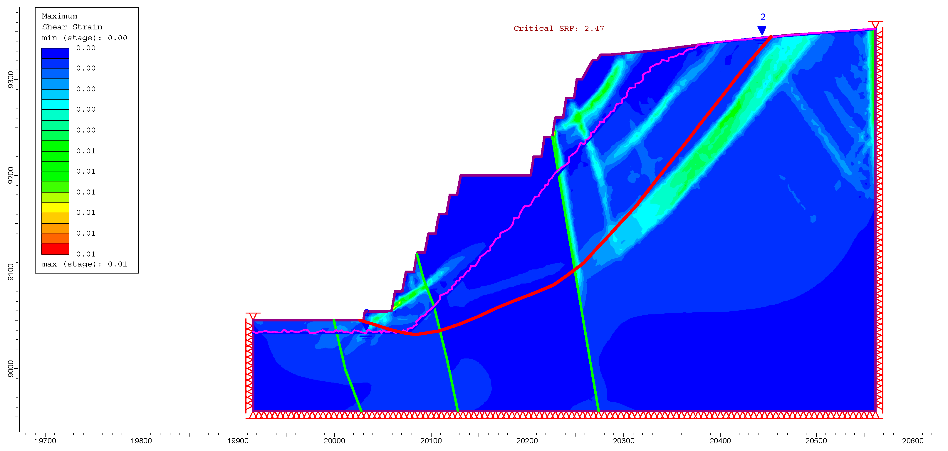
Figure 6 shows the results of the finite element method using the same parameters and model applied in LEM. The critical strength reduction factor (SRF) is 2.47 for the slope. The results show they are in reasonably good agreement with the slip surface assumed in the Spencer LEM analysis. Comparing the results of LEM with SSRM, the factor of safety from LEM is reliable and can be used.
9. Conclusions
In this paper, an overview of probabilistic reliability methods for slope stability calculation considering material uncertainty was presented. The study highlights the need for a conscientious understanding of uncertainty and variability for effective representation of rock slope design. Uncertainty is a common fact in geological engineering problems and three types of uncertainty are normally identified for slope design. These are geological uncertainty related to natural variability in the rock properties, which cannot be reduced no matter our knowledge and expertise displayed in estimating them; model uncertainty related to the possibility of obtaining an incorrect result even if all the exact values are available for all model parameters; and parameter uncertainty related to the inability to account for the various characteristics of the geotechnical model that stem from either data scatter and/or systematic error, such as statistical and bias in measurements. These uncertainties can have a significant impact on the design performance of a slope if not properly accounted for.
There are two main approaches to deal with uncertainties. These are reliability and non-deterministic methods. There are two categories of non-deterministic probabilistic methods and non-probabilistic methods. Probabilistic methods are commonly used to represent and quantify uncertainty in the slope design process. Likewise, the reliability-based design approach quantifies and provides a consistent measure of safety by determining the probability of failure for a slope system. Even though the reliability-based methods may appear complex, they have been logically applied to a variety of rock slope engineering problems. For probability methods, the techniques have been coded in limit equilibrium and finite element computer software. However, as results may differ depending on the reliability (or probability) method chosen, two or more methods should be used to gain an understanding of the errors involved.
A case example was presented to demonstrate the value of probabilistic-based analyses in the slope design process. A rock slope from an open pit in a gold mining operation was studied. Geotechnical parameters are considered significant factors and any inconsistencies in these parameters and difficulty in the selection of appropriate data are paramount in rock slope design. The uniaxial compression strength (UCS), geological strength index (GSI), disturbance factor (D), rock mass constant (mi), and unit weight were determined to be key parameters. UCS and GSI were treated as random variables and a normal distribution was chosen. The Monte Carlo simulation and response surface methods implemented in SLIDE software and solved with cuckoo Spencer limit equilibrium methodology were used for this purpose. The study highlights the need for verification with deterministic finite element methodology in RS2 software. The results were compared and were useful to highlight the benefit of probabilistic analysis of slope designs over the deterministic method.
Geotechnical engineers must be aware that probabilistic slope design methods are evolving and that the deterministic methods are not always consistent slope design methods. They must be aware that when using the deterministic method, significant design errors can occur if the design technique fails to represent the true physical behavior of the slope or rock mass conditions, such as calculating the factor of safety in deterministic limit equilibrium methods or finite element methods. Based on these conditions and for the purposes of expedience, it is necessary to integrate deterministic analysis with probabilistic design analysis to give a credible economic slope design. Slope design methods that use probabilistic analysis give a wider review of failure probability and risk-based decision-making, which is warranted in complex mining situations. Despite their mathematical complexity, the probabilistic-reliability methods discussed are in use today and due to progress in computation, they provide an invaluable reference to decision-making.
Author Contributions
Conceptualization, M.S. and M.A.; methodology, M.A.; software, M.A.; validation, M.A. and M.S.; formal analysis, M.A.; investigation, M.A.; resources, M.A. and M.S.; data curation, M.A.; writing—original draft preparation, M.A.; writing—review and editing, M.S. and M.A.; supervision, M.S.; project administration, M.A. and M.S.; funding acquisition, M.S. Both authors have read and agreed to the published version of the manuscript.
Funding
This research received no external funding.
Acknowledgments
We would like to thank the three anonymous reviewers for the constructive comments and suggestions.
Conflicts of Interest
The authors declare no conflict of interest.
References
- Steffen, O.K.H.; Contreras, L.F.; Terbrugge, P.J.; Venter, J. A Risk Evaluation Approach for Pit Slope Design. In Proceedings of the 42nd U.S. Rock Mechanics Symposium (USRMS), San Francisco, CA, USA, 29 June–2 July 2008. [Google Scholar]
- Ali, M.A.; Morteza, O. Determination and stability analysis of ultimate open-pit slope under geomechanical uncertainty. Int. J. Min. Sci. Technol. 2014, 24, 105–110. [Google Scholar] [CrossRef]
- Zevgolis, I.E.; Deliveris, A.V.; Koukouzas, N.C. Probabilistic design optimization and simplified geotechnical risk analysis for large open pit excavations. Comput. Geotech. 2018, 103, 153–164. [Google Scholar] [CrossRef]
- Obregon, C.; Mitri, H. Probabilistic approach for open pit bench slope stability analysis—A mine case study. Int. J. Min. Sci. Technol. 2019, 29, 629–640. [Google Scholar] [CrossRef]
- Basahel, H.; Mitri, H. Probabilistic assessment of rock slopes stability using the response surface approach—A case study. Int. J. Min. Sci. Technol. 2019, 29, 357–370. [Google Scholar] [CrossRef]
- Santos, T.B.D.; Lana, M.S.; Pereira, T.M.; Canbulat, I. Quantitative hazard assessment system (Has-Q) for open pit mine slopes. Int. J. Min. Sci. Technol. 2019, 29, 419–427. [Google Scholar] [CrossRef]
- Christian, J.T.; Ladd, C.C.; Baecher, G.B. Reliability applied to slope stability analysis. J. Geotech. Eng. 1994, 120, 2180–2207. [Google Scholar] [CrossRef]
- Low, B.K. Reliability analysis of rock wedges. J. Geotech. Geoenviron. Eng. 1997, 123, 498–505. [Google Scholar] [CrossRef]
- Low, B.K. Reliability analysis of rock slopes involving correlated non-normals. Int. J. Rock Mech. Min. 2007, 44, 922–935. [Google Scholar] [CrossRef]
- Park, H.; West, T.R. Development of a probabilistic approach for rock wedge failure. Eng. Geol. 2001, 59, 233–251. [Google Scholar] [CrossRef]
- Jimenez-Rodriguez, R.; Sitar, N.; Chacon, J. System reliability approach to rock slope stability. Int. J. Rock Mech. Min. Sci. 2006, 43, 847–859. [Google Scholar] [CrossRef]
- Johari, A.; Javadi, A.A. Reliability assessment of infinite slope stability using jointly distributed random variable. Sci. Iran. A 2012, 19, 423–429. [Google Scholar] [CrossRef] [Green Version]
- Aladejare, A.E.; Akeju, V.O. Design and Sensitivity Analysis of Rock Slope Using Monte Carlo Simulation. Geotech. Geol. Eng. 2020, 38, 573–585. [Google Scholar] [CrossRef] [Green Version]
- Baecher, G.B.; Christian, J.T. Reliability and Statistics in Geotechnical Engineering; Wiley: Chichester, UK, 2003. [Google Scholar]
- Duzgun, H.S.B.; Yucemen, M.S.; Karpuz, C. A probabilistic model for the assessment of uncertainties in the shear strength of rock discontinuities. Int. J. Rock Mech. Min. Sci. 2002, 39, 743–754. [Google Scholar] [CrossRef]
- Duzgun, H.S.B.; Yucemen, M.S.; Karpuz, C. A methodology for reliability-based design of rock slopes. Rock Mech. Rock Eng. 2003, 36, 95–120. [Google Scholar] [CrossRef]
- Kirsten, H.A.D. Significance of the probability of failure in slope engineering. Civ. Eng. S. Afr. 1983, 25, 17–29. [Google Scholar]
- Rackwitz, R. Reliability analysis—A review and some perspectives. Struct. Saf. 2001, 23, 365–395. [Google Scholar] [CrossRef]
- Miller, S.M.; Whyatt, J.K.; McHugh, E.L.; Australian Geomechanics Society. Applications of Point Estimate Method for Stochastic Rock Slope Engineering. In Proceedings of the Gulf Rocks 2014, 6th North America Rock Mechanics Symposium (NARMS), Houston, TX, USA, 5–9 June 2004; pp. 1–12. [Google Scholar]
- Park, H.J.; West, T.R.; Woo, I. Probabilistic analysis of rock slope stability and random properties of discontinuity parameters. Interstate Highway 40, Western North Carolina, USA. Eng. Geol. 2005, 79, 230–250. [Google Scholar] [CrossRef]
- Duzgun, H.S.B.; Bhasin, R.K. Probabilistic stability evaluation of Oppstadhornet rock slope Norway. Rock Mech. Rock Eng. 2009, 42, 724–749. [Google Scholar] [CrossRef]
- US Army Corps of Engineers. Engineering and Design: Introduction to Probability and Reliability Methods for Use in Geotechnical Engineering; Engineer Technical Letter 1110-2-547; Department of the Army: Washington, DC, USA, 1997. [Google Scholar]
- Reale, C.; Xue, J.; Pan, Z.; Gavin, K. Deterministic and probabilistic multi-modal analysis of slope stability. Comput. Geotech. 2015, 66, 172–179. [Google Scholar] [CrossRef]
- Bastidas-Arteaga, E.; Soubra., A.-H. Doctoral School—Stochastic Analysis and In-Verse Modelling; Reliability Analysis, Methods; Hicks, M.A., Cristina, J., Eds.; HAL Archives-Ouverters: Lyon, France, 2014; pp. 53–77. Available online: http://alertgeomaterials.eu (accessed on 25 May 2021).
- Hasofer, A.M.; Lind, N.C. Exact and invariance second moment code forma. J. Eng. Mech. 1974, 100, 111–121. [Google Scholar]
- Tang, W.H.; Yuecemen, M.S.; Ang, A.H.S. Probability-based short-term design of slopes. Can. Geotech. J. 1976, 13, 201–215. [Google Scholar] [CrossRef]
- Venmarcke, E.H. Reliability of earth slopes. J. Geotech. Eng. Div. 1977, 103, 1227–1246. [Google Scholar]
- Chowdhury, R.N.; Xu, D.W. Geotechnical system reliability of slopes. Reliab. Eng. Syst. Saf. 1995, 47, 141–151. [Google Scholar] [CrossRef]
- Low, B.K.; Tang, W.H. Efficient reliability evaluation using spreadsheet. J. Eng. Mech. 1997, 123, 749–752. [Google Scholar] [CrossRef]
- Low, B.K.; Gilbert, R.B.; Wright, S.G. Slope reliability analysis using generalized method of slices. J. Geotech. Geoenviron. Eng. 1998, 124, 350–362. [Google Scholar] [CrossRef]
- Low, B.K. Practical probabilistic slope stability analysis. Proc. Soil. Rock Am. 2003, 2, 2777–2784. [Google Scholar]
- Cho, S.E. Probabilistic stability analyses of slopes using the ANN-based response surface. Comput. Geotech. 2009, 36, 787–797. [Google Scholar] [CrossRef]
- Low, B.K. FORM, SORM, and spatial modeling in geotechnical engineering. Struct. Saf. 2014, 49, 56–64. [Google Scholar] [CrossRef]
- Fenton, G.A.; Griffiths, D.V. Risk Assessment in Geotechnical Engineering; Wiley: Hoboken, NJ, USA, 2008. [Google Scholar]
- Chowdhury, R.N.; Xu, D.W. Rational polynomial technique in slope stability analysis. J. Geotech. Eng. 1993, 119, 1910–1928. [Google Scholar] [CrossRef]
- Dai, Y.; Fredlund, D.G.; Stolte, W.J. A probabilistic slope stability analysis using deterministic computer software. In Probabilistic Methods in Geotechnical Engineering; CRC Press: Canberra, Australia, 1993; pp. 267–274. [Google Scholar]
- El-Ramly, H.; Morgenstern, N.R.; Cruden, D.M. Probabilistic slope stability analysis for practice. Can. Geotech. J. 2002, 39, 665–683. [Google Scholar] [CrossRef]
- Park, H.J.; Jeong, U.J.; Han, B.H.; Ro, B.D.; Shin, K.H.; Kim, J.K. The evaluation of the probability of rock wedge failure using the point estimate method and maximum likelihood estimation method. In Proceedings of the 10th IAEG International Congress, Nottingham, UK, 6–10 September 2006; p. 485. [Google Scholar]
- Park, H.J.; Um, J.G.; Woo, I.; Kim, J.W. The evaluation of the probability of rock wedge failure using the point estimate method. Environ. Earth Sci. 2011, 65, 353–361. [Google Scholar] [CrossRef]
- Xu, B.; Low, B.K. Probabilistic stability analyses of embankments based on finite-element method. J. Geotech. Geoenviron. Eng. 2006, 132, 1444–1454. [Google Scholar] [CrossRef]
- Zhang, J.; Zhang, L.M.; Tang, W.H. Slope reliability analysis considering site-specific performance information. J. Geotech. Geoenviron. Eng. 2011, 137, 227–238. [Google Scholar] [CrossRef]
- Tobutt, D.C. Monte Carlo simulation methods for slope stability. Comput. Geosci. 1982, 8, 199–208. [Google Scholar] [CrossRef]
- Husein Malkawi, A.I.; Hassan, W.F.; Abdulla, F.A. Uncertainty and reliability analysis applied to slope stability. Struct. Saf. 2000, 22, 161–187. [Google Scholar] [CrossRef]
- McMahon, B.K. A Statistical Method for the Design of Rock Slopes. In Proceedings of the 1st Australia-New Zealand Conference on Geomechanics, Melbourne, Australia, 9 August 1971; pp. 314–321. [Google Scholar]
- McMahon, B.K. Geotechnical Design in the Face of Uncertainty; Memorial Lecture; Davis, E.H., Ed.; Australian Geomechanics Society: Sydney, Australia, 1985. [Google Scholar]
- Chowdhury, R.N. Geomechanics risk model for multiple failures along rock discontinuities. Int. J. Rock Mech. Min. Sci. Geomech. Abstr. 1986, 23, 337–346. [Google Scholar] [CrossRef]
- Genske, D.D.; Walz, B. Probabilistic assessment of the stability of rock slopes. Struct. Saf. 1991, 9, 179–195. [Google Scholar] [CrossRef]
- Low, B.K.; Einstein, H.H. Simplified Reliability Analysis for Wedge Mechanisms in Rock Slopes. In Proceedings of the 6th International Symposium on Landslides, Rotterdam, The Netherlands, 10 February 1992; pp. 499–507. [Google Scholar]
- Madsen, H.O.; Krenk, N.C. Methods of Structural Safety; Prentice Hall: Hoboken, NJ, USA, 1986. [Google Scholar]
- Melchers, R.E. Structural Reliability Analysis and Predictions, 2nd ed.; Wiley: Chichester, UK, 1996. [Google Scholar]
- Straub, D. (Ed.) Reliability and Optimization of Structural Systems, 1st ed.; CRC Press: Boca Raton, FL, USA, 2010. [Google Scholar] [CrossRef]
- Bishop, A.W. The use of the slip circle in the stability analysis of earth slope. Geotechnique 1995, 5, 7–17. [Google Scholar] [CrossRef]
- Samui, P.; Kumar, R.; Yadav, U.; Kumari, S.; Bui, D.T. Reliability Analysis of Slope Safety Factor by Using GPR and GP. Geotech. Geol. Eng. 2019, 37, 2245–2254. [Google Scholar] [CrossRef]
- Griffiths, D.V. Stability Analysis of Highly Variable Soils by Elasto-Plastic Finite Elements (1999); Phase2 user’s guide Version 2.1; Rocscience Inc.: Toronto, ON, Canada, 2002. [Google Scholar]
- Schweiger, H.F.; Peschl, G.M. Reliability analysis in geotechnics with the random set finite element method. Comput. Geotech. 2005, 32, 422–435. [Google Scholar] [CrossRef]
- Read, J. Data Uncertainty: Guidelines for Open Pit Slope Design; Read, J., Stacey, P., Eds.; CSIRO Publishing: Clayton, Australia, 2009; pp. 214–220. [Google Scholar]
- Bedi, A.; Harrison, J.P. Characterisation and Propagation of Epistemic Uncertainty in Rock Engineering: A Slope Stability Example. In Proceedings of the International Symposium of the ISRM, Wroclaw, Poland, 21–26 September 2013. [Google Scholar]
- Abdulai, M.; Sharifzadeh, M. Uncertainty and reliability analysis of open pit rock slopes: A critical review of methods of analysis. Geotech. Geol. Eng. 2019. [Google Scholar] [CrossRef]
- Abbaszadeh, M.; Shahriar, K.; Sharifzadeh, M.; Heydari, M. Uncertainty and reliability analysis to slope stability: A case study from Sungun Copper Mine. Geotech. Geol. Eng. 2011, 29, 581–596. [Google Scholar] [CrossRef]
- Langford, J.C.; Diederichs, M.S. Application of Reliability Methods in Geological Engineering Design. In Proceedings of the Pan-Am Canadian Geotechnical Conference, Toronto, ON, Canada, 2–6 October 2011. [Google Scholar]
- Zadeh, L.A. Fuzzy sets. Inf. Control 1965, 8, 338–353. [Google Scholar] [CrossRef] [Green Version]
- Shrestha, B.; Duckstein, L. A fuzzy reliability measure for engineering applications. In Uncertainty Modeling and Analysis in Civil Engineering; CRC Press: Boca Raton, FL, USA, 1998; pp. 121–135. [Google Scholar]
- Tonon, F.; Bernardini, A.; Mammino, A. Determination of parameters range in rock engineering by means of random set theory. Reliab. Eng. Syst. Saf. 2000, 70, 241–261. [Google Scholar] [CrossRef]
- Tonon, F.; Bernardini, A.; Mammino, A. Reliability analysis of rock mass response by means of random set theory. Reliab. Eng. Syst. Saf. 2000, 70, 263–282. [Google Scholar] [CrossRef]
- Peschl, G.M. Reliability Analyses in Geotechnics with the Random Set Finite Element Method. Ph.D. Thesis, Institute for Soil Mechanics and Foundation Engineering, Graz University of Technology, Graz, Austria, 2004. [Google Scholar]
- Shen, H. Non-Deterministic Analysis of Slope Stability Based on Numerical Simulation. Ph.D. Thesis, Freiberg University of Mining and Technology, Freiberg, Germany, 2012. [Google Scholar]
- Low, B.K.; Tang, W.H. Reliability analysis using object-oriented constrained optimization. Struct. Saf. 2004, 26, 68–89. [Google Scholar] [CrossRef]
- Cornell, C.A. First-Order Uncertainty Analysis of Soils Deformation and Stability; University of Hong Kong Press: Hong Kong, China, 1971; pp. 129–144. [Google Scholar]
- Duncan, J.M. Factors of safety and reliability in geotechnical engineering. J. Geotech. Geoenviron. Eng. 2000, 126, 307–316. [Google Scholar] [CrossRef]
- Christian, J.T. Geotechnical engineering reliability: How well do we know what we are doing? J. Geotech. Geoenviron. Eng. 2004, 130, 985–1003. [Google Scholar] [CrossRef]
- Rackwitz, R.; Fiessler, B. Structural reliability under combined random load sequences. Comput. Struct. 1978, 9, 489–494. [Google Scholar] [CrossRef]
- Breitung, K. Asymptotic approximations for multinormal integrals. ASCE J. Eng. Mech. 1984, 110, 357–366. [Google Scholar] [CrossRef] [Green Version]
- Zhang, J.; Du, X. A second-order reliability method with first-order efficiency. J. Mech. Des. 2010, 132, 1–8. [Google Scholar] [CrossRef]
- Dadashzadeh, N.; Duzgun, H.S.B.; Gheibi, S. A Second-Order Reliability Analysis of Rock Slope Stability in Amasya, Turkey. In Proceedings of the 13th International ISRM Congress, International Symposium on Rock Mechanics, Montreal, QC, Canada, 10–13 May 2015. [Google Scholar]
- Der Kiureghian, A.; De Stefano, M. Efficient algorithm for second-order reliability analysis. J. Eng. Mech. 1991, 117, 2904–2927. [Google Scholar] [CrossRef]
- Zhao, Y.G.; Ono, T. New approximations for SORM: Part 1. J. Eng. Mech. 1999, 125, 79–85. [Google Scholar] [CrossRef] [Green Version]
- Zhao, Y.G.; Ono, T. Moment methods for structural reliability. Struct. Saf. 2001, 23, 47–75. [Google Scholar] [CrossRef]
- Tvedt, L. Two Second Order Approximations to the Failure Probability; Veritas Report DIV/20-004-83; Det Norske Veritas: Bærum, Norway, 1983. [Google Scholar]
- Rosenblueth, E. Point Estimates for Probability Moments. Proc. Natl. Acad. Sci. USA 1975, 72, 3812–3814. [Google Scholar] [CrossRef] [Green Version]
- Rosenblueth, E. Two-point estimates in probabilities. Appl. Math. Model. 1981, 5, 329–335. [Google Scholar] [CrossRef]
- Langford, J.C. Application of Reliability Methods to the Design of Underground Structures. Ph.D. Thesis, Queen’s University, Kingston, ON, Canada, 2013. [Google Scholar]
- Langford, J.C.; Diederichs, M.S. Quantifying uncertainty in Hoek-Brown intact strength envelopes. Int. J. Rock Mech. Min. Sci. 2015, 74, 91–102. [Google Scholar] [CrossRef]
- Tsai, C.W.; Franceschini, S. Evaluation of probabilistic point estimate methods in uncertainty analysis for environmental engineering applications. J. Environ. Eng. 2005, 131, 387–395. [Google Scholar] [CrossRef]
- Wang, Y.; Cao, Z.; Au, S.K. Practical reliability analysis of slope stability by advanced Monte Carlo simulations in a spreadsheet. Can. Geotech. J. 2011, 48, 162–172. [Google Scholar] [CrossRef]
- Gibson, W. Probabilistic methods for slope analysis and design. Aust. Geomech. 2011, 46, 29. [Google Scholar]
- Hammah, R.E.; Yacoub, T.E.; Curran, J.H. Probabilistic Slope Analysis with the Finite Element Method. In Proceedings of the 43rd US Rock Mechanics Symposium and 4th US-Canada Rock Mechanics Symposium, Asheville, NC, USA, 28 June–1 July 2009. [Google Scholar]
- Shamekhi, E.; Tannant, D.D. Probabilistic assessment of rock slope stability using response surfaces determined from finite element models of geometric realizations. Comput. Geotech. 2015, 69, 70–81. [Google Scholar] [CrossRef] [Green Version]
- Hill, W.J.; Hunter, W.G. A review of response surface methodology: A literature survey. Technometrics 1966, 8, 571–590. [Google Scholar] [CrossRef]
- Sayed, S.; Dodagoudara, G.R.; Rajagopala, K. Finite element reliability analysis of reinforced retaining walls. Geomech. Geoeng. 2010, 5, 187–197. [Google Scholar] [CrossRef]
- Zhang, J.; Huang, H.W.; Phoon, K.K. Application of the Kriging-based response surface method to the system reliability of soil slopes. J. Geotech. Geoenviron. 2013, 139, 651–655. [Google Scholar] [CrossRef]
- Li, D.Q.; Jiang, S.H.; Cao, Z.J.; Zhou, W.; Zhou, C.B.; Zhang, L.M. A multiple response surface method for slope reliability analysis considering spatial variability of soil properties. Eng. Geol. 2015, 187, 60–72. [Google Scholar] [CrossRef]
- Li, D.; Chen, Y.; Lu, W.; Zhou, C. Stochastic response surface method for reliability analysis of rock slopes involving correlated non-normal variables. Comput. Geotech. 2011, 38, 58–68. [Google Scholar] [CrossRef]
- Bucher, C.G.; Bourgund, U. A fast and efficient response surface approach for structural reliability problems. Struct. Saf. 1990, 7, 57–66. [Google Scholar] [CrossRef]
- Rocscience Inc. Slide Version 7.0-2D Limit Equilibrium Slope Stability Analysis; Rocscience Inc.: Toronto, ON, Canada, 2015; Available online: www.rocscience.com (accessed on 7 June 2021).
- Choi, S.K.; Grandhi, R.V.; Canfield, R.A.; Pettit, C.L. Polynomial chaos expansion with latin hypercube sampling for estimating response variability. AIAA J. 2004, 42, 1191–1198. [Google Scholar] [CrossRef]
- Yang, X.S.; Deb, S. Cuckoo Search via Lévy Flights. In Proceedings of the 2009 World Congress on Nature & Biologically Inspired Computing (NaBIC), Coimbatore, India, 9–11 December 2009; pp. 210–214. [Google Scholar] [CrossRef]
- Wu, A. Locating General Failure Surfaces in Slope Analysis via CUCKOO Search. 2012. Available online: https://www.rocscience.com/help/slide2/pdf_files/theory/Cuckoo_Search.pdf (accessed on 21 May 2021).
- Gandomi, A.H.; Yang, X.S.; Talatahari, S.; Alavi, A.H. Metaheuristic Algorithms in Modeling and optimization. In Metaheuristic Applications in Structures and Infrastructures; Elsevier: Amsterdam, The Netherlands, 2013; pp. 1–24. [Google Scholar] [CrossRef]
- Azizi, M.A.; Marwanza, I.; Hartanti, N.A.; Ghifari, M.K.; Anugrahadi, A. Application of Cuckoo Search Method in 3D Slope Stability Analysis for Limestone Quarry Mine. Indones. Min. J. 2020, 23, 57–65. [Google Scholar]
- McQuillan, A.; Canbulat, I.; Oh, J.; Gale, S.; Yacoub, T. Case Study: Comparing Slide3 Models to Actual Slope Failure in an Open Cut Coal Mine. 2018. Available online: https://www.rocscience.com/documents/pdfs/rocnews/2018spring/Slide3CaseStudy.pdf (accessed on 10 June 2021).
- Mohamad, A.B.; Zain, A.M.; Bazin, N.E.N. Cuckoo Search Algorithm for Optimization Problems—A Literature Review and its Applications. Appl. Artif. Intell. 2014, 28, 419–448. [Google Scholar] [CrossRef]
- Yang, X.S.; Deb, S. Engineering optimisation by cuckoo search. Int. J. Math. Model. Numer. Optim. 2010, 1, 330–343. [Google Scholar] [CrossRef]
- Eberhart, R.; Kennedy, J. New Optimizer Using Particle Swarm Theory. In Proceedings of the 6th International Symposium on Micro Machine and Human Science, Nagoya, Japan, 4–6 October 1995; pp. 39–43. [Google Scholar]
- Kennedy, J.; Eberhart, R. Particle Swarm Optimization. In Proceedings of the IEEE International Conference on Neural Networks, Perth, WA, Australia, 27 November–1 December 1995; pp. 1942–1948. [Google Scholar]
- Shi, Y.; Eberhart, R.C. Empirical Study of Particle Swarm Optimization. In Proceedings of the 1999 Congress on Evolutionary Computation-CEC99 Cat, Washington, DC, USA, 6–9 July 1999. [Google Scholar]
- Eberhart, R.C.; Shi, Y. Particle Swarm Optimization: Developments, Application and Resources. In Proceedings of the 2001 Congress on Evolutionary Computation (IEEE Cat. No.01TH8546), Seoul, Korea, 27–30 May 2001; pp. 81–86. [Google Scholar]
- Wang, G.; Sun, F.; Tang, Q. Reliability Analysis of Rock Slope Excavation Considering the Stochasticity and Finite Persistence of Wedges. Period. Polytech. Civ. Eng. 2018, 62, 660–669. [Google Scholar] [CrossRef] [Green Version]
- Gholizadeh, S.; Salajegheh, E. Optimal design of structures subjected to time history loading by swarm intelligence and an advanced metamodel. Comput. Methods Appl. Mech. Eng. 2009, 198, 2936–2949. [Google Scholar] [CrossRef]
- Li, Y.; Tian, Y.; Oyang, Z.; Wang, L.; Xu, T.; Yang, P.; Zhao, H. Analysis of soil erosion characteristics in small watersheds with particle swarm optimization, support vector machine, and artificial neuronal networks. Environ. Earth Sci. 2010, 60, 1559–1568. [Google Scholar]
- Poitras, G.; Lefrançois, G.; Cormier, G. Optimization of steel floor systems using particle swarm optimization. J. Constr. Steel Res. 2011, 67, 1225–1231. [Google Scholar] [CrossRef]
- Kuok, K.K.; Harun, S.; Shamsuddin, S.M. Particle swarm optimization feedforward neural network for hourly rainfall runoff modeling in Bedup Basin, Malaysia. Int. J. Civ. Environ. Eng. 2010, 9, 9–18. [Google Scholar]
- Kuok, K.K.; Harun, S.; Shamsuddin, S.M. Particle swarm optimization feedforward neural network for modeling runoff. Int. J. Environ. Sci. Technol. 2010, 7, 67–78. [Google Scholar] [CrossRef] [Green Version]
- Chen, B.R.; Feng, X.T. CSV-PSO and Its Application in Geotechnical Engineering. In Swarm Intelligence: Focus on Ant and Particle Swarm Optimization; Chan, F.T.S., Tiwari, M.K., Eds.; BoD—Books on Demand: Norderstedt, Germany, 2007; pp. 263–288. [Google Scholar]
- Bharat, T.V.; Sivapullaiah, P.V.; Allam, M.M. Swarm intelligence-based solver for parameter estimation of laboratory through-diffusion transport of contaminants. Comput. Geotech. 2009, 36, 984–992. [Google Scholar] [CrossRef]
- Yazdi, J.S.; Kalantary, F.; Yazdi, H.S. Calibration of soil model parameters using particle swarm optimization. Int. J. Geomech. 2012, 12, 229–238. [Google Scholar] [CrossRef]
- Zhao, H.B.; Zou, Z.S.; Ru, Z.L. Chaotic particle swarm optimization for non-circular critical slip surface identification in slope stability analysis. In Boundaries of Rock Mechanics Recent Advances and Challenges for the 21st Century: Proceedings of the International Young Scholars’ Symposium on Rock Mechanics, Beijing, China, 28 April–2 May 2008; CRC Press: Boca Raton, FL, USA; pp. 585–588.
- Cheng, Y.M.; Li, L.; Sun, Y.J.; Au, S.K. A coupled particle swarm and harmony search optimization algorithm for difficult geotechnical problems. Struct. Multidiscip. Optim. 2012, 45, 489–501. [Google Scholar] [CrossRef]
- Kalatehjari, R.; Ali, N.; Kholghifard, M.; Hajihassani, M. The effects of method of generating circular slip surfaces on determining the critical slip surface by particle swarm optimization. Arab. J. Geosci. 2014, 7, 1529–1539. [Google Scholar] [CrossRef]
- Kalatehjari, R.; Safuan, A.; Rashid, A.; Ali, N.; Hajihassani, M. The Contribution of Particle Swarm Optimization to Three-Dimensional Slope Stability Analysis. Sci. World J. 2014, 2014, 973093. [Google Scholar] [CrossRef] [PubMed] [Green Version]
- Jiang, J.C.; Yamagami, T.; Baker, R. Three-dimensional slope stability analysis based on nonlinear failure envelope. Chin. J. Rock Mech. Eng. 2003, 22, 1017–1023. [Google Scholar]
- Cheng, Y.M.; Li, L.; Chi, S.C. Performance studies on six heuristic global optimization methods in the location of critical slip surface. Comput. Geotech. 2007, 34, 462–484. [Google Scholar] [CrossRef]
- Javadzadeh, E.; Javadzadeh, R. Bishop’s Simplified Method and Particle Swarm Optimization for Location the Critical Failure Surface in Rock Slope Stability Analysis. In Proceedings of the ISRM International Symposium—5th Asian Rock Mechanics Symposium (ARMS5), Tehran, Iran, 24–26 November 2008. [Google Scholar]
- Millonas, M.M. Swarms, Phase Transitions, and Collective Intelligence. In Computational Intelligence: A Dynamic System Perspective; IEEE Press: Piscataway, NJ, USA, 1994; pp. 137–151. [Google Scholar]
Figure 1.
Types of uncertainty.


Figure 3.
Illustration of the linear and nonlinear limit state function [58].
Figure 3.
Illustration of the linear and nonlinear limit state function [58].

Figure 4.
Illustration of the probability density function (PDF) showing the reliability index β and probability of failure pf for a performance function of a system.
Figure 4.
Illustration of the probability density function (PDF) showing the reliability index β and probability of failure pf for a performance function of a system.

Figure 5.
Probabilistic limit equilibrium slope stability analysis.

Figure 6.
Result of deterministic finite element analysis.


| Reliability Index β | Probability of Failure Pf =Φ(−β) | Expected Performance Level |
|---|---|---|
| 1.0 | 0.16 | Hazardous |
| 1.5 | 0.07 | Unsatisfactory |
| 2.0 | 0.023 | Poor |
| 2.5 | 0.006 | Below average |
| 3.0 | 0.001 | Above average |
| 4.0 | 0.00003 | Good |
| 5.0 | 0.0000003 | High |
Where Φ(−β) = standard normal cumulative distribution function.
Table 2.
Input parameters of the rock material.
| Rock Type | Unit Weight (kN/m3) | Generalized Hoek–Brown | ||||||||
|---|---|---|---|---|---|---|---|---|---|---|
| UCS (MPa) | GSI | mi | D | Young’s Modulus (GPa) | Poisson Ratio | σUCS (MPa) | σGSI | Distribution | ||
| Volcaniclastic Sediment | 27.4 | 140 | 58 | 24 | 1.0 | 2.78 | 0.3 | 34.5 | 13.3 | Normal |
| Basalt | 28.8 | 168 | 68 | 25 | 1.0 | 4.93 | 0.2 | 32.0 | 10.0 | Normal |
| Porphyry | 26.3 | 215 | 60 | 20 | 1.0 | 3.34 | 0.2 | 53.9 | 12.0 | Normal |
Table 3.
Result of FoS and PoF from limit equilibrium analysis.
| Probability Method | FS | PF (%) | RI |
|---|---|---|---|
| MCS | 2.587 | 0 | 3.2 |
| RSM | 2.902 | 0.2 | 2.7 |
MCS = Monte Carlo Simulation; RSM = Response Surface Method; FS = Factor of Safety; PF = Probability of Failure; RI = Reliability Index.
Publisher’s Note: MDPI stays neutral with regard to jurisdictional claims in published maps and institutional affiliations. |
© 2021 by the authors. Licensee MDPI, Basel, Switzerland. This article is an open access article distributed under the terms and conditions of the Creative Commons Attribution (CC BY) license (https://creativecommons.org/licenses/by/4.0/).
Share and Cite
MDPI and ACS Style
Abdulai, M.; Sharifzadeh, M. Probability Methods for Stability Design of Open Pit Rock Slopes: An Overview. Geosciences 2021, 11, 319. https://0-doi-org.brum.beds.ac.uk/10.3390/geosciences11080319
AMA Style
Abdulai M, Sharifzadeh M. Probability Methods for Stability Design of Open Pit Rock Slopes: An Overview. Geosciences. 2021; 11(8):319. https://0-doi-org.brum.beds.ac.uk/10.3390/geosciences11080319
Chicago/Turabian StyleAbdulai, Musah, and Mostafa Sharifzadeh. 2021. "Probability Methods for Stability Design of Open Pit Rock Slopes: An Overview" Geosciences 11, no. 8: 319. https://0-doi-org.brum.beds.ac.uk/10.3390/geosciences11080319
Note that from the first issue of 2016, this journal uses article numbers instead of page numbers. See further details here.