1. Introduction
After the boom of the previous decade, natural gas has reestablished itself as a valuable resource for years to come in the United States (US). The increased use of natural gas has resulted in more infrastructure and more potential for methane losses along the supply chain from producers to consumers. These losses have serious environmental consequences as the main component of natural gas is methane, a greenhouse gas (GHG) with a higher global warming potential (GWP) than carbon dioxide (CO
2). The International Panel on Climate Change (IPCC) determined that the GWP of methane was 28 over 100 years and 84 over 20 years [
1]. According to the Environmental Protection Agency (EPA), methane made up over 10% of all US GHG emissions from human activities and over 16% of all global GHGs in 2017 on a CO
2 equivalent basis [
2]. The International Energy Agency (IEA) estimated that there were 79 million tons of methane emissions from the oil and gas industry in 2018 worldwide [
3].
Several studies have raised issues with these national inventories, as they tend to underestimate emissions. Miller et al. [
4] estimated that US methane emissions reported by the EPA were up to 1.5 times lower than actual values. Brandt et al. [
5] conducted an extensive review of published estimates in 2011 and concluded that emissions from the natural gas infrastructure were 1.25–1.75 times higher than EPA estimates. National estimates of emissions have typically relied on a small number of direct quantification measurements intended to be representative of a national population. Direct quantification techniques may have relatively low measurement uncertainty, but have high personnel and monetary costs, require site access, and only represent emissions at a single point in time. The latter resulting in uncertainties because emissions are known to vary temporally [
6,
7]. As such, measurements made during direct quantification efforts may not be representative of long-term averages. If the prescribed emissions factors or measurements were not representative at the time of measurement, then errors were propagated to national estimates. Recent works have focused on improved technologies for methane measurement and methods for quantification. The Department of Energy’s (DOE) Advanced Research Projects Agency—Energy (ARPA-E) invested in the development of commercially viable solutions for accurate methane measurement [
8,
9]. Recent research has also focused on the development of more accurate, indirect measurement methods for continuous emissions monitoring [
10,
11,
12,
13]. Improvements in technologies and methods would allow for more accurate quantification of emissions, long-term, on a site level with reduced time, cost and labor. While these measurements may not be available at every site, a better understanding of average site variation, can improve models and estimates, in combination with periodic direct measurements. These methods often rely on continuous monitoring from stationary points. Other test method (OTM) 33A is one such method [
14,
15]. It has been widely used to estimate methane emissions indirectly from natural gas sites [
15,
16,
17].
OTM 33A was developed by the EPA under the Office of Research and Development (ORD) as a general guide for geospatial measurement of air pollution (GMAP). The emissions quantification (EQ) assessment method under OTM 33A was developed for application to emissions sources that were near ground level, relatively small in area and within 150 meters (m) of the measurement location. The OTM 33A EQ method is addressed in our research and is simply referred to as OTM 33A herein. In the design of the method, the developers assumed that the instrumentation used for measurement was mounted to a vehicle and because of this, best practices were defined with respect to road (rather than site) access. Several factors required for effective use of OTM 33A included:
An accessible downwind roadway from the source;
A relatively consistent wind condition blowing from the source to the point of measurement;
Zero or few obstructions between the source and the measurement point;
A source near ground level;
Little or no other nearby sources in addition to the target source [
14].
OTM 33A required measurements of 3D wind speed, typically with a sonic anemometer, gas concentration measurement with parts per billion (ppb) granularity and atmospheric pressure and temperature. A concentration measurement instrument (CMI) should sample at a point close to the wind speed measurement location. The method recommended collecting data at a rate of at least one Hertz (Hz) and prescribed multiple measurements be taken under these conditions, each ranging in time from 15–20 min [
14]. A range finder was recommended to estimate the distance from the source to the measurement location, as a distance estimate was necessary for calculations [
16].
Several studies have examined the accuracy of OTM 33A with controlled-release experiments. The controlled releases of the studies presented here used methane as the controlled release. The initial releases, performed by the EPA, took place alongside the development of the method. The original test matrix consisted of 107 observations each spanning 20 min. Releases were conducted in flat open fields at various locations. The bulk of the measurements were made with sensor and source heights of 2.7 m and 3.1 m, respectively. The release rates of the study ranged from 0.19 g/s to 1.2 g/s. Most the releases (59%) were 0.6 g/s. Distances varied between 18 m and 179 m; the average distance from release to sensor was approximately 70 m. The method produced an initial accuracy that ranged from −84% to 184% [
16]. After periods of data that did not meet the primary data-quality indicators (DQI) were removed, 74% of measurements remained. The errors of these measurements ranged from −60% to 52%, however, 71% of measurements were within ±30% of the actual release rate [
17].
Robertson et al. [
17] performed controlled-release experiments at Christman Airfield (CAF) in Fort Collins, CO. This series of experiments consisted of 23 tests with distances between 30 m and 175 m and release rates ranging from 0.03 g/s to 0.56 g/s. Nineteen of the 23 data periods met the DQI requirements. Robertson et al. combined their results with those from the EPA, which yielded a dataset of 119 tests. These data had a 2σ error of ±56%, a 1σ error of ±28% and around a 10% low bias.
A more recent study by Edie et al. [
18] further investigated the controlled-release experiments of Robertson et al. [
17], along with new data collected at the Methane Emissions Technology Evaluation Center (METEC) in Fort Collins, CO. Where the CAF data set focused on the effectiveness of OTM 33A in an open area with a single known source location. The METEC set was conducted with the potential for multiple releases from different components at a mock natural gas production site. The study observed that across both test sets wind speed, number of sources, and release height had no major impact on estimate accuracy.
Table 1 contains the details of these two studies.
An ordinary least squares regression analysis confirmed the 10% low bias seen by Robertson et al. and a propensity to overestimate smaller releases. Edie et al. concluded that OTM 33A measurements had a 2σ error of ±70% with a slight negative bias [
18].
Robertson et al. and Brantley et al. have used the OTM 33A to estimate emissions from well pads in various natural gas basins [
16,
17]. Both studies employed bootstrapping methods to attempt to enhance the confidence of estimates made from the method. Robertson et al.’s measurements were compared to onsite, direct measurements by Bell et al. using a variance weighted least squares (VWLS) approach [
19]. The average distance of these measurements was 46 ± 24 m. The study concluded that OTM 33A underestimated emissions based on the VWLS approach applied to sites where the onsite estimate was composed primarily of direct measurements, although estimates by onsite measurements and OTM 33A were within uncertainties at 65% of sites.
The purpose of this study was to investigate the potential to use OTM 33A as a long-term monitoring method and improve the mechanistic understanding of results obtained from such a method.
2. Data Acquisition and Analysis
In our work, OTM 33A data were collected continuously while several controlled methane releases were performed. The data were evaluated using various data collection rates, period lengths, and wind filters (WF). OTM 33A calculations were then performed on contiguous periods with known release rates and distances.
Measurements were conducted at the West Virginia University JW Ruby Research Farm [
20]. The farm was selected due to its openness and lack of high canopy vegetation or building interference. The release experiments took place in an open grass field that was normally used for cattle grazing. The farm was not perfectly flat, with slight rolling hills, which resulted in differences in altitude based on positioning. While cattle were not present in the field of the setup, there were cattle in the area which may have contributed to elevated background methane emissions.
Assessment of the OTM 33A method was performed with controlled-release experiments. Previous studies on indirect mobile quantification used controlled release test distances between 5 m and 179 m [
16,
17,
18]. The controlled release distances of this work were designed to be representative of a deployment of the system at an active well site. Distances were estimated on site using a range finder but were later calculated based on more accurate GPS coordinates and ranged from 42 to 119 m. Release rates from previous studies ranged from 0.03 g/s to 1.2 g/s [
16,
17,
18]. The controlled release rates of this work were 0.04 g/s, 0.12 g/s and 0.24 g/s.
Tables S1 and S2 provide the details of the entire controlled release matrix including calculated distances from GPS coordinates.
Methane releases were produced from a three-bottle manifold of technical to high purity methane (98–99% composition by volume) connected in parallel to a mass flow controller (MFC). The MFC was stored in a trailer on-site and was powered with a 12 V battery. The MFC was capable of controlling methane flow up to 0.24 g/s ± 0.0024 g/s [
21]. The outlet of the MFC was at atmospheric pressure and was connected to a length of tubing with an inner diameter of 25 mm that was attached to the top of the trailer, simulating a release from an onsite blunt body, such as a tank. This yielded a methane release height of approximately 2.3 m.
The data acquisition (DAQ) equipment used for measurements consisted of a LICOR LI-7700 CH
4 analyzer for methane concentration, temperature and pressure and a Gill
® WindMaster 3-axis sonic anemometer for wind speed. The LI-7700 was open path and utilized wavelength modulation spectroscopy (WMS) to measure methane concentrations from 0–40 ppm with a resolution of 5 ppb [
22]. The WindMaster was a 3-axis sonic anemometer capable of measuring wind speed from 0 to 50 m/s with a resolution of 0.01 m/s in three directions corresponding to a standard rectangular coordinate system [
23]. Additional system components included a LICOR LI-7500DS CO
2/H
2O analyzer, an Omega iBTHx and a LI-COR LI-220R pyranometer [
24,
25,
26]. Methane and wind speed measurements were recorded at a rate of 10 Hz.
Table S3 presents complete specifications of the instruments.
The DAQ equipment was attached to a 4-m-high tower that was mounted on a towable trailer. The absolute sample height was approximately 4.5 m. DAQ setups of this kind have been used for a method of gas flux measurement known as eddy covariance. The equipment was powered by a rechargeable battery bank maintained by two solar panels, also mounted on the trailer. The system is presented in
Figure S1.
Data were recorded over the course of 114 days between May 21, 2019 and September 11, 2019. During this time, useful data were recorded on 92 of the days. The days that did not include data collection were due to analyzer replacement, equipment failure and logistical conflictions. Of the 92 days there were 42 containing some period with a controlled methane release present. Days in which no release was performed (50) were considered “background”. Data loss during these 92 days was due to natural phenomenon that inhibited the open path analyzer operation; including rain, fog or other path interference and was considered “functional data loss”.
The emissions rate calculated from OTM 33A was governed by a Gaussian curve fit of average concentrations binned by wind direction. This inverse quantification technique is commonly referred to as point source Gaussian (PSG). To determine the Gaussian fit, the methane concentration data were grouped by wind direction bins of 10° increments and data in each bin were averaged. The bin with the maximum concentration was shifted to the center for curve fitting. The average background concentration (defined as the lowest 5% of data measured during the period) was subtracted from each bin to produce an average elevated concentration. The horizontal and vertical dispersion coefficients were determined from the atmospheric stability indicator (ASI), defined as a value between 1 and 7. These stability indicators were similar to the classic Pasquill stability classes and were determined by a combination of the turbulence intensity (TI) and standard deviation of the horizontal wind direction [
16]. TI was defined as the standard deviation of the vertical wind speed divided by the average horizontal wind speed. The details of the calculations were found in the source code for OTM 33A as available online [
14]. OTM 33A estimations were calculated with a script written in Python 3.6 [
27]. This code was based on a 2015 version of the published OTM 33A MATLAB
® code (120415_Histcount.m) [
14,
28]. The Python results were validated with 10 Hz data collected by the EPA [
14]. The only difference was that 3D sonic anemometer local wind speed averages were used (this analysis) rather than a local meteorological station’s 2D wind data (original OTM analysis) for the purpose of stability classification. This change was made because there were no continuous data available from a weather station near the data collection site. The change affected results in 4 of the 20 original cases evaluated. The differences were due to a change in identified stability class.
Table S4 presents the differences in the two calculations. Two of the four results had a difference greater than 40% because of this change. This analysis demonstrated the sensitivity of such methods to minor changes in variables used to determine stability class. While the method for estimating stability class may not impact most measurements (75%), different methodologies have the potential to change estimated emissions rates by up to 50%. This sensitivity to stability class was also noted during the original development of OTM 33A [
14].
3. Results
The results presented here were determined based on the data collection previously described. Baseline OTM 33A results used a period length of 20 min and a data collection rate of 10 Hz, as is recommended by the EPA. OTM 33A also suggested binning parameters which include bin size, bin angle cut limit, bin percent cut limit, background percentage and wind speed limit. For the purpose of the analyses performed here these values were kept at their recommended default values of 10, 60, 2, 5 and 0, respectively.
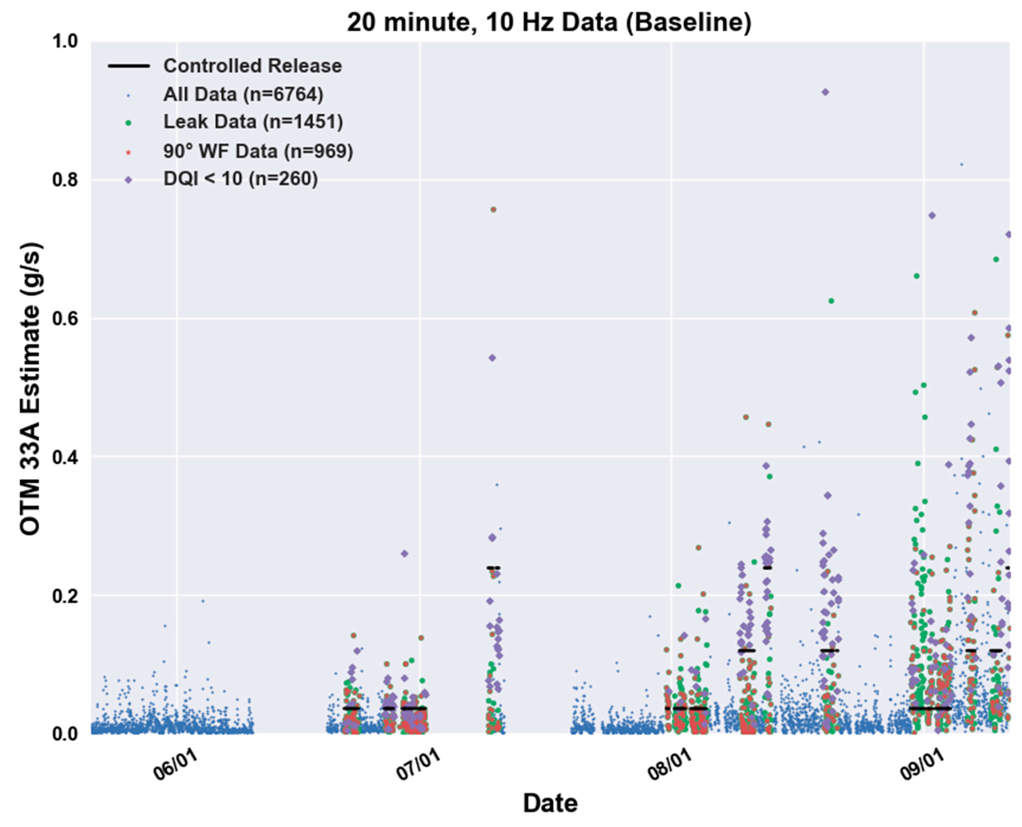
To reduce data from 10 Hz to various other frequencies a forward averaging technique was applied. For example, the first point of a 1 Hz period was an average of the first ten measurements of 10 Hz data. During data collection there were a total of 1451 20-min periods in which OTM 33A estimates were calculated and a controlled release was present. Without any wind filter (all data were included whether the mean wind direction was “release to tower” or not) the root mean squared error (RMSE) of the dataset was 0.139 g/s and the normalized root mean square deviation (NRMSD) was 177%. The definitions of these values are presented in
Equations S1 and S2. However, this dataset had little value for the purpose of the current analysis, as it included periods when the wind was blowing from “tower to release”, pushing the released gas away from the measurement point. To eliminate these periods, the data were filtered to include only those periods that had a mean wind direction within ±90° of the direction from the controlled release to the DAQ tower. This would be representative of placing a vehicle downwind of the site when using the traditional OTM 33A method. The wind filter is presented visually in
Figure S2 and the mathematically in Equation S3. This reduced the number of periods evaluated to 921, the RMSE to 0.121 g/s and the NRMSD to 148%. This was “the baseline dataset” as it was the most simplified version of data that could be considered to have any validity. All evaluations performed were also performed with a ±90° wind filter, except when the filter itself was varied. No other exclusions were made. Data are presented in
Figure 1 along with controlled release rate.
To determine the optimal wind filter, various angles were evaluated. The wind filter used to determine the data used in evaluations was varied to determine an optimal range. Results of the evaluation indicated that a ±60° limit may be the optimal filter for the difference in wind direction and release-to-tower direction. This wind filter was applied to the dataset during the other evaluations performed and when applied to all baseline results reduced the RMSE to 0.117 g/s. Note that OTM 33A stated that an important DQI was that the fitted concentration within ±30° of the source direction. However, this is a different filter than that used in the DQI. The maximum concentration bin could be within ±30° of the source direction even if the mean wind direction during that time was outside ±30°.
Table 2 presents the results of the various wind filters.
The analysis conducted on period length and data frequency were filtered by the ±60° wind filter. The data were evaluated based on different period lengths. OTM 33A recommended a period of 15–20 min. Period lengths used for evaluation included 10, 15, 20, 25, 30, 45 and 60 min. The same wind filter was applied to the data and other binning parameters remained constant.
Table 3 presents the results of the period length evaluation and indicates that based on RMSE the most effective period length was 25 min which resulted in a RMSE of 0.111 g/s. Data frequency effects were also evaluated. Seven different data rates were used in the evaluation. Raw data were collected at a rate of 10 Hz, but window averaged values were used to reduce the data processing frequency. It should be noted that the downsampling method could impact results, using an average of the window will have a general “smoothing” effect on the data, whereas selecting every n
th point would not. Future research will explore the effects of different downsampling methodologies.
Table 4 presents the results of the data frequency evaluation and indicates that a 0.2-Hz or 5-s average frequency was the most effective with an RMSE of 0.106 g/s. Results separated by controlled release rate are presented in
Tables S5–S7.
The findings here suggested that the optimal evaluation would be a period length of 25 min and a data frequency of 0.2 Hz, filtered by a wind angle difference of ±60°. Results of this optimized dataset are presented in
Table 5. The data in
Table 5 is also separated by controlled release rate and the NRMSD is presented.
Typically, OTM 33A evaluations were filtered by a DQI less than 10. The baseline dataset was filtered by this DQI value, reducing the sample size to 260 periods. The DQI filtered data are presented in
Figure 1. DQI filtering caused an increase in RMSE from 0.121 to 0.134 g/s. The RMSE only decreased in four of the nine individual scenarios in the controlled release matrix, when compared to the baseline dataset. DQI filtering did improve the RMSE on average at the two higher release rates of 0.12 and 0.24 g/s. Robertson et al. [
17] used a category rating system to distinguish between levels of DQI acceptability. They stated that a DQI less than five was considered “Category 1” or the best evaluations. The periods with a DQI value below five were limited to 110 and resulted in a RMSE of 0.124 g/s. When comparing DQI filters, those periods with a rating less than five had a lower RMSE on average across all release rates than those with a rating less than 10. Periods with a rating less than five again decreased RMSE in six of the nine scenarios. However, when evaluating the entire dataset, the ±60° wind filter alone produced a lower RMSE (0.117 g/s), than “Category 1” DQI periods (RMSE = 0.124 g/s). When applying both the optimal wind filter and a DQI limit of ten to the entire dataset, the number of periods available was reduced to 217, but caused an increase in RMSE to 0.141 g/s, worse than the DQI or wind filtering alone. The optimized dataset (presented in
Table 5) resulted in a lower RSME (0.093 g/s) than any other evaluated dataset filtered from the baseline dataset. The number of periods evaluated and their respective RMSE values for the discussed scenarios are presented in
Table 6.
Figure 2 presents box and whisker plots of the scenarios discussed.
Red dotted lines in
Figure 2 represent median values, blue dashed lines represent mean values, the box represents the upper and lower quartiles and the whiskers represent the 5th and 95th percentiles of the data. Note that those filters that included DQI tended to give a positive percent error (overestimate), while using wind filter alone tended to underestimate release rates.
Some trends were observed during the analysis of periods, data rates and wind filters with respect to distance. The trends were analyzed by distance rather than release rate due to the fact that in a real world scenario, the user could obtain estimates of distance to potential fugitive emissions a priori but would have no insight into the mass rate of those emissions. Estimated distance had a near linear relationship with OTM 33A estimates (R2 = 0.97), across all evaluations. This was because estimated distance was a direct multiplier in the standard PSG equation.
The same analysis as described above was used. To evaluate results sorted by the distance from the releases to the DAQ tower. It is important to note that the results compared at various distances were not the same data with a different distance measurement but were completely different data periods. Since wind directions during various distance measurements varied, the sample size of the data analyzed were different for each scenario. The three approximate distances analyzed were ~50, 75 and 120 m. The exact distances are presented in
Table S1. Some noteworthy trends by distance included the following:
Across all analyses, the RMSE tended to increase linearly with distance on average (R2=0.92);
DQI filtering (<10) showed few trends across distances. DQI filtered data only improved RMSE compared to the baseline dataset at the middle distance. “Category 1” improved RMSE at the shortest distance (<60 m) by 4% but resulted in a 32% increase in RMSE at the furthest distance (~120 m);
When analyzing period length, the default 20-min length did not produce the lowest RMSE at any distance;
For the nearest distances (<60 m) tighter wind filters (±30°, ±20°) and longer periods (45, 60 min) gave the smallest RMSEs.
The optimal parameters for various distances are presented in
Table 7. A complete matrix of distance sorted data are presented in
Table S5.
4. Optimized Dataset Discussion
It is noteworthy that the overall optimal combination of period length, wind filter and data frequency occurred at the maximum distance. This could be because larger distances from source to measurement location have greater potential to produce more erroneous results. Comparisons were made by varying one parameter at a time and evaluating the dataset based on RMSE. When evaluating the effect of period length, RMSE was minimized with the use of 25-min periods across the full range of scenarios evaluated. When evaluating data rate, a frequency of 0.2 Hz produced the lowest RMSE. When different wind filters were applied to the complete dataset, RMSE was minimized by filtering out all periods where the difference between the “release to tower” and mean wind directions was greater than ±60°. OTM 33A results with these three parameters were evaluated and produced a RMSE of 0.093 g/s. This was lower than any other RMSE evaluated in from the baseline analyses of
Table 2,
Table 3 and
Table 4.
Delving deeper into the optimized dataset presented different trends than those of the default dataset. The RMSE of the ±60° wind filter of the optimized dataset was greater than that of using the baseline ±90° and a ±30° wind filters by 3.2% and 2%, respectively with the optimal period length and data rate. While this difference is minor it suggests that the optimal wind filter could be dependent upon other variables. The DQI results were more positive on the optimized dataset. The standard DQI filter of 10 did not improve the RMSE of the optimized dataset without combining it with a wind filter. However, when the DQI filter was used in combination with the ±60° wind filter the resultant RMSE of 130 evaluations was 0.084 g/s. Category 1 DQI filtering (DQI < 5) without a wind filter resulted in a RMSE of 0.077 g/s, but limited the number of evaluations to 70. This suggests that when searching for optimal parameters they may differ for various distances, emission rates, and atmospheric conditions. There was concern over whether the reduction in RMSE of these scenarios was due to the fact that the number of evaluations was reduced, however, across all evaluations performed in this work, presented in
Table 2,
Table 3 and
Table 4, there was no discernable correlation between the number of evaluations and RMSE (21 evaluations, R
2 < 0.001). Overall, the optimized dataset with a ±60° wind filter allowed for 50% of periods to be evaluated and produced a RMSE of 0.093 g/s and NRMSD of 105%. This is an improvement in all aspects compared to standard OTM 33A period, frequency and DQI below ten, which allowed only 18% of periods to be evaluated and produced a RMSE of 0.134 g/s and a NRMSD of 122%.
While inconclusive from this work alone, the distance-based results suggest that different parameters may be optimal at different distances. When the distance between the release and the point of data collection is less than 60 m it may be better to use longer periods for analysis and a tighter wind filter. Such an approach may lead to improved confidence, but a smaller number of evaluations (N). Some fields of study such as eddy covariance base their averaging time on atmospheric conditions. The differing optimal period lengths may not be a function of distance, but instead of the conditions experienced during measurement. Further investigation into period length in combination with other binning parameters, wind filters and data rating systems may produce different optimal parameters for different atmospheric conditions.
In addition, there was no investigation here into the binning parameters used in the OTM 33A analysis. The variables of bin size, bin angle cut limit, bin percent cut limit and methane background percentage all impact the Gaussian curve fit used to estimate the release rate. The wind speed limit could eliminate periods where there were insignificant atmospheric conditions for effective plume transport, which is critical to the success of PSG methods. These variables should be investigated. There is also the potential that optimization of parameters is interdependent. If this is the case, the optimized combinations of the parameters evaluated, as well as the binning parameters may improve results. The optimization of parameters could also depend on other factors such as the general time of year, stability class or other atmospheric conditions. Future research will explore the possibilities of optimized parameters under different atmospheric conditions.
5. Conclusions
Better understanding of methane emissions from the natural gas sector requires more knowledge of temporal variability. This knowledge is difficult to obtain through direct measurements. Continuous monitoring has the potential to fill gaps in data, provided that methods can be improved and uncertainty reduced. Optimizing a method of data evaluation may produce results with less uncertainty. Contiguous data analysis with an optimized method could reduce the uncertainty of individual measurements and give more confidence to researchers and industry seeking to better understand the temporal nature of emissions.
The purpose of the analyses performed here was to evaluate the use of OTM 33A as a continuous monitoring method. Optimization of parameters can enhance the mechanistic understanding of using PSG methods for long term data collection.
The results here suggested that different period lengths, wind filters, data acquisition frequencies and data quality filters impacted method accuracy when applied to long term measurements. DQI tended to improve results for optimized scenarios, however, there may be cases when a simple wind filter is more effective in eliminating deficient data. Optimal period length and data frequency may be a function of transport variables such as wind speed and distance. For example, this study suggested that when data collection was performed at distances less than 70 m that longer averaging periods may be useful. Downsampling data may result in smoother averages for PSG curve fitting which may enhance periods of data with consistent atmospheric conditions. It was also clear that parameters must be optimized concurrently. While some parameters can improve results when others are held constant, the optimized dataset (25-min periods, 0.2-Hz frequency, ±60° wind filter) produced a higher RMSE (0.093 g/s) than using the same period and frequency and the baseline ±90° wind filter (RMSE = 0.090 g/s). To optimize variables globally a more extensive matrix of release rate and distance scenarios should be evaluated. Another important variable was the atmospheric conditions of the site being measured. For example, the atmospheric conditions during these data collection period allowed a ±60° wind filter to capture 50% of available periods. Filtering by DQI less than ten only captured 18% of available periods. Evaluation of period length, data rate, wind filter, data quality filter, and OTM 33A binning parameters simultaneously will allow for higher confidence of these long-term measurements. This in turn may enable improved methods and understanding of temporal variability of methane emissions.

 ,
, 


