Investigating Spatiotemporal Variability of Water, Energy, and Carbon Flows: A Probabilistic Fuzzy Synthetic Evaluation Framework for Higher Education Institutions

Abstract

Higher education institutions (HEIs) consume significant energy and water and contribute to greenhouse gas (GHG) emissions. HEIs are under pressure internally and externally to improve their overall performance on reducing GHG emissions within their boundaries. It is necessary to identify critical areas of high GHG emissions within a campus to help find solutions to improve the overall sustainability performance of the campus. An integrated probabilistic-fuzzy framework is developed to help universities address the uncertainty associated with the reporting of water, energy, and carbon (WEC) flows within a campus. The probabilistic assessment using Monte Carlo Simulations effectively addressed the aleatory uncertainties, due to the randomness in the variations of the recorded WEC usages, while the fuzzy synthetic evaluation addressed the epistemic uncertainties, due to vagueness in the linguistic variables associated with WEC benchmarks. The developed framework is applied to operational, academic, and residential buildings at the University of British Columbia (Okanagan Campus). Three scenarios are analyzed, allocating the partial preference to water, or energy, or carbon. Furthermore, nine temporal seasons are generated to assess the variability, due to occupancy and climate changes. Finally, the aggregation is completed for the assessed buildings. The study reveals that climatic and type of buildings significantly affect the overall performance of a university. This study will help the sustainability centers and divisions in HEIs assess the spatiotemporal variability of WEC flows and effectively address the uncertainties to cover a wide range of human judgment.

1. Introduction

Benchmarks are set by many educational sectors to report energy consumption to communicate their performances. For example, typical energy consumption benchmarks for 320 educational buildings in Europe were reported to be 87 kWh/m² in Greece, 197 kWh/m² in Flanders, and 119 kWh/m² in Northern Ireland [1]. In the UK and Wales, educational buildings were found to be the most homogenous among all the non-domestic buildings, with a median of 46 kWh/m² for schools and 74 kWh/m² for HEIs [2]. Hernandez et al. (2008) benchmarked 88 non-domestic educational buildings in Ireland and ranked their performance in seven classes from (A–G) based on their energy performances [1]. Water benchmarks in educational buildings are less common than energy. The US educational buildings consume around 6% of the public sector’s water usage, e.g., water consumption in nine large educational buildings is about 133 million m³ per year which is equivalent to 0.595 m³/m² [3]. Water is less monitored as it has been reported that university buildings do not report water consumption per building for most of their buildings [4]. Alghamdi et al. (2020) benchmarked water consumption in 71 academic buildings and reported that water usage intensity (water used per area) for 50th and 75th percentile are 0.85 m³/m² and 1.26 m³/m² [5] in Canadian HEIs. Water may be involved directly and indirectly in generating electricity and consequently a factor in emitting GHG emissions. For example, water is directly involved in hydroelectric power plants and indirectly involved in thermal power plants, where steam is used in rotating turbines and water is used in cooling the steam [6]. Furthermore, due to the thermo-physical properties, water may be used as a thermally bonding agent to transfer energy in geothermal plants. Energy usage directly produces GHG emissions because of the combustion of fuels (e.g., natural gas) and upstream processes (e.g., reservoirs and transportation) in hydroelectricity. Therefore, when benchmarking GHG emissions, it is necessary to specify the types of energy use to determine the actual impact of an HEI on its environment.

Sustainability assessment is a challenging task, due to its inter-disciplinary nature [7]. Many of the reporting systems and theories carry inherent uncertainties. Gasparatoes et al. (2008) carried out a critical review of sustainability assessment tools and methodologies and concluded that none of the metrics reviewed seem to assess progress towards sustainability in a holistic manner [8]. The tools reviewed include the biophysical models and indicator-based reporting systems, such as the exergy (maximum potential work attainable), energy (total direct and indirect energy available required to make a service or a product), and sustainability indicators (SI) have underlying uncertainties [8]. These indicators are aggregated to deliver a judgment rank of sustainability heavily influenced by the weights of indicators [9].

Building rating tools, such as the Leadership in Energy and Environmental Design (LEED) certifications, are among the tools that carry significant uncertainties. Agdas et al. (2015) assessed the energy performance of 10 LEED certified academic buildings and 14 non-LEED buildings at the University of Florida. They concluded that no statistically significant differences between the two types of buildings. In fact, the energy usage intensity (EUI) is slightly higher in LEED classified buildings than those not certified [10]. Reporting is needed to communicate sustainability, and to do this, the uncertainties associated with the ranks, judgment, and data limitations, need to be addressed for more accurate assessment outcomes [11]. It was also reported that some HEIs, such as the University of Alberta, received a gold rating in the Sustainability Tracking, Assessment, and Reporting System (STARS), even though it has reported a substantial increase in GHG emissions over the years [5].

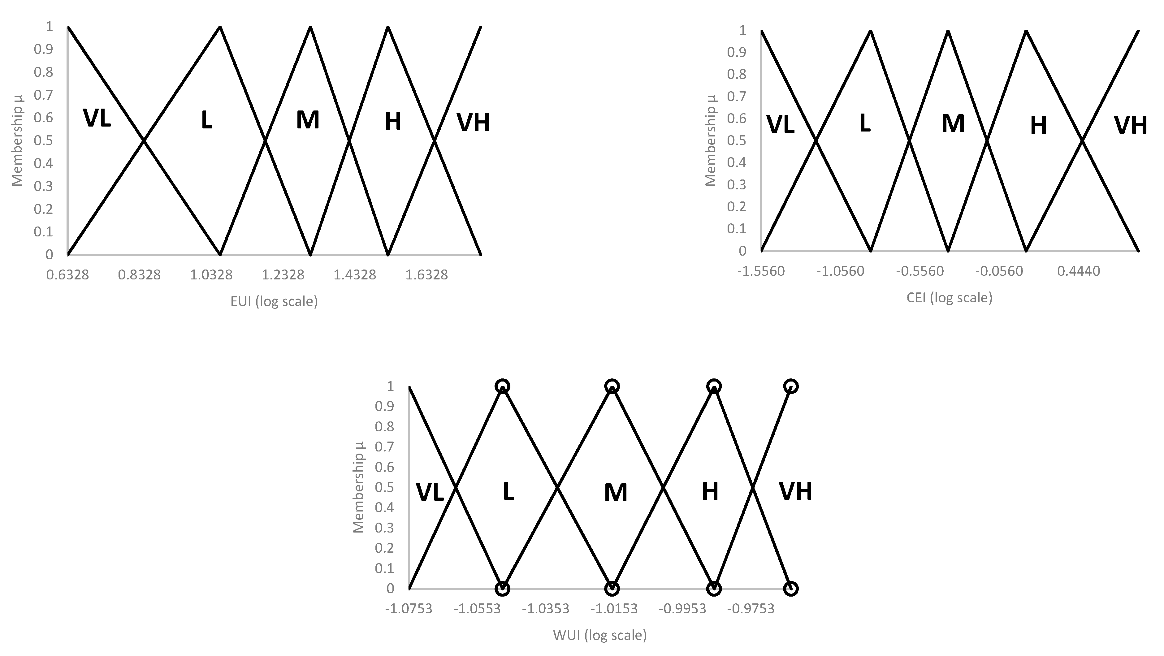
There are two types of uncertainties in reporting sustainability assessment results: Aleatory and epistemic uncertainties [12]. The aleatory uncertainties are generated from the random variation of data and are addressed using probabilistic techniques, such as Monte Carlo simulations, and the epistemic uncertainties are due to the lack of the knowledge vagueness that is a result of using linguistic scoring systems, such as rankings like Gold, Silver, or LEED-certified, and so on [13]. The vagueness of linguistic variables can be addressed using fuzzy set-based techniques [14]. These reporting systems aggregate the scores of indices and provide an overall rating—for instance, the STARS reporting system awards a HEIs a Bronze if the minimum score is 25, silver is below 45, and so on. Credits in the reporting systems cover the full spectrum of sustainability, and the reporting system has bonus scores for some criteria. Some of the credits assessed did not apply to all HEIs [15]. In addition to these uncertainties, the uncertainties associated with occupants’ energy use behaviors in educational buildings are another type of challenge in emission reduction [16].

Despite the significant environmental impacts posed by HEIs, this sector has the least amount of data available for performance assessment [17]. The data gap becomes a significant obstacle in communicating, planning, monitoring, verifying, and even managing the WEC flows. This may be due to the limited technical and financial resources HEIs possess, specifically in small to medium-sized universities [18]. The data gap will lead to uncertainty in the results. Fuzzy techniques have been applied in assessing the sustainability of academic buildings. Alghamdi et al. (2020) assessed singe yearly averages performances of 71 academic buildings in two campuses in two different climatic regions of British Columbia, Canada using fuzzy clustering analysis [5]. Santamouris (2007) used fuzzy clustering techniques to address the uncertainty related to classification in energy benchmarks in schools in Greece [19]. Chung (2006) used fuzzy linear regression to classify and benchmark commercial buildings [20]. Haider et al. (2018) used fuzzy synthetic evaluation to assess sustainability in a small neighborhood [14]. A combination of probabilistic and fuzzy synthetic evaluation has been reported in other risk assessment studies [12,21,22]. These studies assessed the performance of HEIs building using averages of singular years without addressing random uncertainties. A rigorous data collection effort is needed to assess the performance of HEIs over several years. The past studies provided a point-based evaluation in a single year and did not include variability of climatic or occupant trends. Furthermore, these studies did not address the volatility, uncertainty, complexity, and ambiguity (VUCA) in current benchmarking techniques [23].

2. Background

The United Nations Paris Agreement set an ambitious goal to keep global temperature rise within 1.5 °C by 2030 to restrict signatory parties from increasing the release of (GHG) [24]. Today, the curb on emissions is facing daunting challenges [25]. The agreement called upon nations to reduce their GHG emissions by committing to an intended nationally determined contributions (INDC), which are unilateral pledges made by the countries, collectively and individually, to reduce their overall GHG emissions [26]. These INDC targets that once seem attainable are now pushed further to 2040, 2050, and beyond. The agreement has not been a successful model for implementing measurable changes to reduce anthropogenic GHG emissions [27]. To overcome the challenges associated with the agreement, reporting mechanisms have been put under review. Some researchers proposed methods to overcome certain socio-economic challenges imposed by the agreement; for instance, Liu et al. (2017) proposed a metabolic capitalized assessment of emissions through a sectorial full-supply chain [28]. Although similar proposals may be viewed as a reductionist approach (i.e., to view sustainability from a single dimension) to sustainability, they underlay a set of considerations in people’s opinions and judgment. They are also an important attempt to improve the current mechanisms of decision making in the process [8].

Buildings consume large amounts of primary and secondary sources of energy. Electricity and heat generation are the largest contributors to GHG emissions and are the most challenging to address. As of 2018, this sector was responsible for nearly 43% of the global GHG emissions, followed by the use of transportation, industry, residential, commercial, public service sectors [29]. The building sector in the united states accounts for 76% of the electricity usage and nearly 40% of the primary energy and associated GHG emissions [30]. In Greece, the building sector consumes 36% of the country’s energy consumption [31]. Energy consumption of non-domestic buildings accounts for nearly 24% of the total energy consumption in China [32]. In addition to the significant usage of energy, the growth in energy consumption in the building sector is estimated to rise by 50% in the next three decades [17]. As a result of high energy usage, buildings are responsible for more than a third of the total GHG emissions globally [33]. In the UK, building energy generation accounts for 19% of the UK’s emissions [34]. The Canadian building sector is the third-largest GHG emitting source, responsible for 12% of the nation’s total emissions [35]. Buildings emit most of the emissions during the operational phase of their life cycle [36]. Furthermore, the growth in GHG emissions from the building sector resulting from the increased energy consumption is alarming. For instance, Greece’s GHG emissions growth is at 4% per annum [31].

In Canada, educational buildings are grouped under the nation’s largest category, the commercial and institutional sector (C&I). This sector consumes 12% of the nation’s entire energy and is responsible for 11% of the nation’s emissions [37]. Educational buildings are significant emission contributors, due to their high energy consumption [38]. The operational buildings in HEIs consume a vast amount of energy to generate flows that are crucial to meet the requirements of the livable indoor environment. As a result, these buildings produce a significant amount of GHG emissions onsite. They are also responsible for harmful impacts on the environment, such as water resource depletion. Brown and Southworth (2008) reported that buildings are responsible for 43% of the GHG emissions in the US [39]. Faulconbridge (2013) reported a 70% increase in anthropogenic gases in urban areas like London than rural areas resulting from building operations [40]. The extent of the impact of this sector is the least understood to date [41]. A 2004 study on 351 HEIs in Canada, reported that (i) academic buildings consume 50 GJ of energy and emit nearly 2.7 MtCO₂e, (ii) universities on average consume 2.04 GJ/m², (iii) colleges consumed 1.48 GJ/m² [42]. Furthermore, this sector heavily depends on fossil fuels for its primary and secondary energy sources, with 65% of energy is supplied by natural gas and other fuels [42]. This is consistent with reports that indicate that HEIs in china consume 30 million tons of standard coal to meet their energy demands [43]. Academic buildings were found to consume more energy, water, and release carbon compared to other types of buildings on campus [5]. The educational sector in the US spends $7.5 billion on energy in a year; this cost is among the highest expenses the educational sector bears. Due to the limited resources, HEIs face challenges in implementing operational needs, preventative maintenance, and adapt efficient interventions, which often leads to deteriorating equipment and results in high energy costs and environmental impacts [44]. A global increase in energy costs is another challenge faced by HEIs [17].

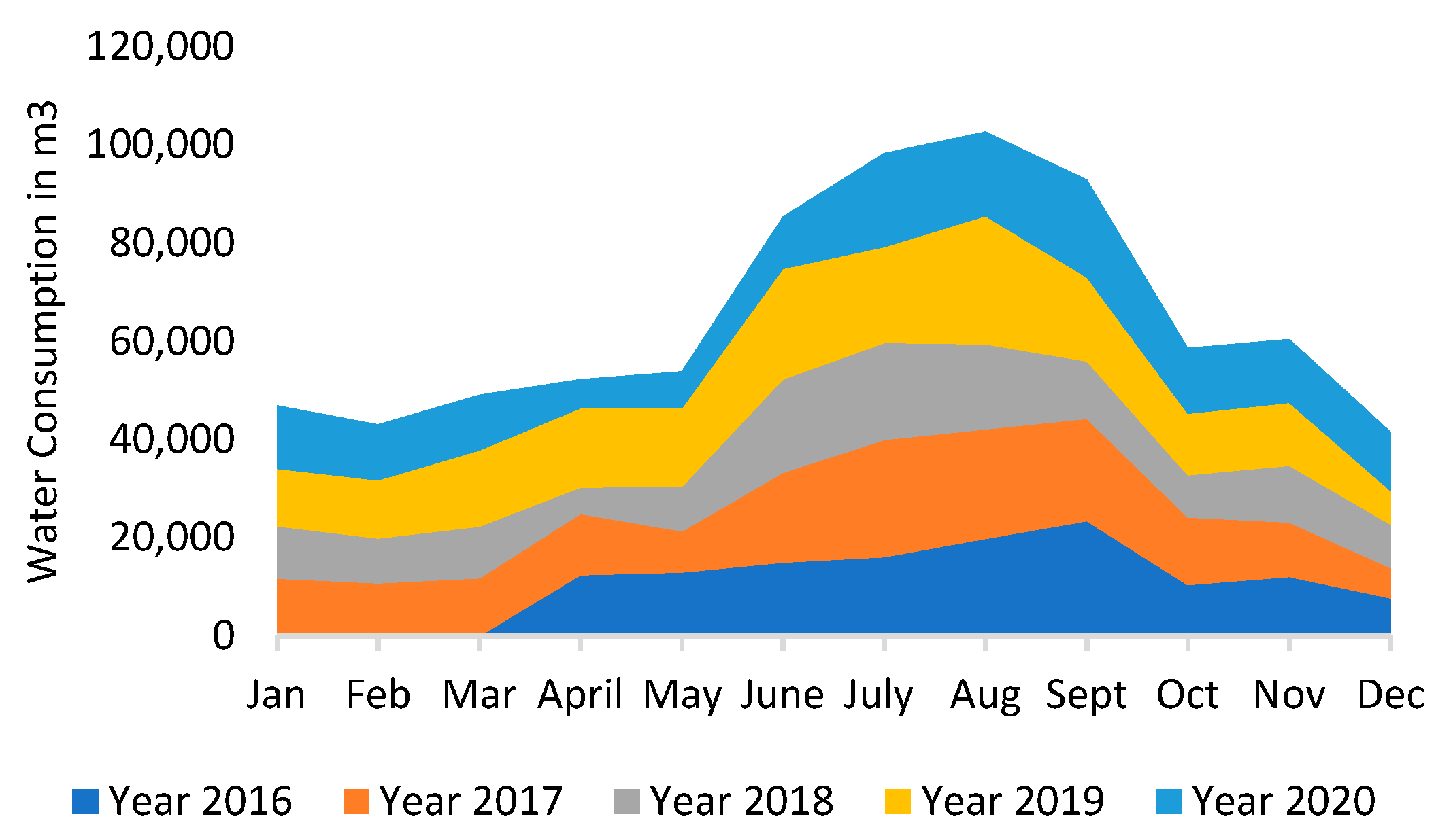
Water undergoes several processes depending on the nature of the water source. In BC, the typical processes are extraction, treatment, distribution, use, and disposal [45]. Different steps involved in these processes use energy and simultaneously emit emissions into the environment. Calculating the entire emissions on the campus needs to take all these steps (all over the water lifecycle) into considerations. This interconnection between water, energy, and carbon (WEC), specifically for the irrigation water used for green areas of a university, will be referred to as the water–energy–carbon (WEC) nexus.

Have complex infrastructure that includes buildings, pumping stations, green spaces, recreational facilities, residential buildings, and operation buildings, HEIs operate like small cities [46]. With 40% consumption of the energy devoted to the public sector, the Chinese HEIs are considered the largest emitter in the entire public sector [47]. The HEIs in British Columbia (Canada) consume 60% of the educational sector energy [42] of the entire province and produce 19% of the total public sector GHG emissions [48]. Water consumption per student in China is found to double that of the average citizen in the country [43]. In the US, educational buildings use 6% of the total public sector water usage [49]. Several studies highlighted water, energy, and carbon challenges of HEIs: In Canada [5], Australia [16], UK [50], China [51], Spain [52], Nigeria [17] Saudi Arabia [53], Poland [54] USA [55], Malaysia [56], Portugal [57], and Norway [58].

HEIs buildings have unique characteristics compared to other types of buildings. First, the growth rates in these institutions are fairly visible. In China, the total floor area of campus buildings grew five times between 1998 and 2011 [43]. In the UK, enrollment is found to increased 33% over a ten-year period between 1996–2005 [59]. Second, energy assessment of HEIs is challenging, due to the uncertainties associated with the occupants’ energy use behavior [16]. For instance, it is reported that the number of users entering and exiting a university building in an hour is equal to the maximum occupancy of those buildings [60]. Another study reported that 92% of the occupants in a university building are visitors [34]. Furthermore, floor area is among many prediction variables used to estimate energy consumption in HEI buildings [61]. Due to these uncertainties, it is believed that energy demand in these buildings is the least understood among all non-domestic buildings [62]. Finally, the energy consumption performance deteriorates with time, due to several building envelopes and HVAC units operating in HEIs [63]. Furthermore, many HEIs buildings were constructed before energy codes were applicable [41]. It is reported that 55% of commercial building (including HEI buildings) projects prior to the construction did not model energy in their design process, and do not adhere to any code compliance or green certification [30]. Therefore, monitoring, reporting, and continuous improvements are needed in HEIs.

Managing the adverse impacts associated with HEIs operations is necessary, due to the intrinsic role of HEIs in leading research, fostering talent, and creating safe and livable neighborhoods [64]. Emission estimation for educational buildings is challenging because energy demands in educational buildings are the least understood among the non-residential buildings, due to their highly variable demand behaviors [10]. Some researchers highlighted the impact of occupancy behavior on energy consumption in buildings [65], while others have reported that the occupancy patterns do not significantly impact energy demand [34]. To promote energy conservation and sustainable use of energy, the European energy performance of building directive proposed reporting as means to effectively assess the institutions’ performances. For example, the UK introduced laws to increase awareness in improving a buildings’ energy performance, which require buildings to report and benchmark their energy consumption performances [66].

Reporting carbon emissions is a legal requirement for many HEIs, due to its role in calculating the carbon taxation imposition. However, HEIs do not consider carbon sequestration as means to mitigate the carbon released from their operations. Carbon sequestration includes both biological (in the form of plantation) and mechanical (in the form of carbon capture technologies) mechanisms and calculates the amount of carbon absorbed by the trees, shrubs, turfs, and soil in a campus. It is believed that carbon sequestration to have a significant impact at the community level [67]. A detailed carbon sequestration calculation involves both the type and area of vegetation.

Sustainability Reporting (SR) can be defined as the formal act of communicating the social, environmental, and financial performances of an organization [68]. The primary aim of the SR is to meet the demands of industrial growth, causing minimum impacts on the environment. This definition embodies the generalized theme of sustainable development (SD) stated by the Word Commission on Environment and Development as one that “meets the needs of the present without compromising the ability of future generations to meet their own needs [69]”. The SR has become a normative practice among HEIs to meet sustainable development goals. Many reporting systems use indicators as the primary tool to make cross-institutional comparations (i.e., benchmarking) [53]. For instance, Martin (2005) stressed the need for developing techniques that can help in advancing SD in universities by using indicators and suggested that ecological footprint could be a useful approach for universities to report their performance [70].

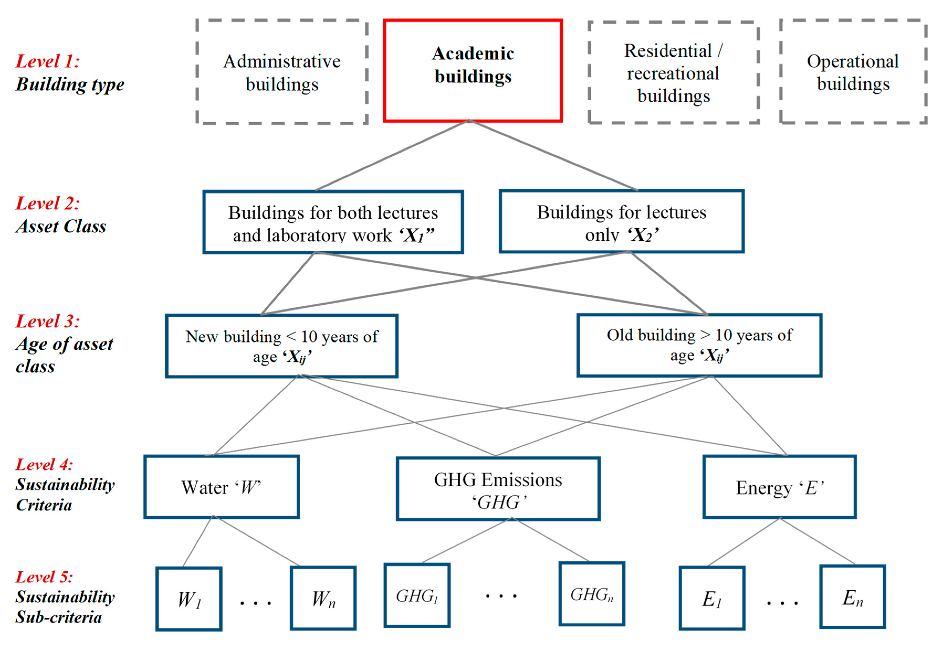
The objective of this study is to propose a framework to assess the spatiotemporal variability in the sustainability of HEIs in terms of water use, energy use, and carbon emissions, incorporating probabilistic and linguistic uncertainties. This paper also proposes a method to estimate and include carbon sequestration by HEIs’ greenery in a campus sustainability rating system for the first time.

3. Methodology

3.1. Evaluation of Water, Energy, and Carbon Emissions

Figure 1 presents the developed probabilistic-fuzzy synthetic evaluation framework (PFSEF) to assess buildings’ performance in terms of WEC flows. The framework consists of three modules, including Module 1: The selection and calculation of indicators, Module 2: Probabilistic assessment, and Module 3: Fuzzy synthetic evaluation assessment. Performance indicators are used to assess water use, energy use, and carbon emissions. The GHG emissions were calculated using the carbon equivalency of each source of energy. The biological carbon sequestration (negative emission) on campus was also estimated for the irrigation activities. The normalized WEC flows per building were then calculated. The probabilistic assessment addresses the aleatory uncertainties with the WEC data collection. The outcomes were then processed in a fuzzy synthetic system to accommodate the uncertainties in linguistic variables that are commonly used in benchmarking. A scenario analysis addressed the preferences to WEC. The fuzzy system consists of a fuzzy set and a fuzzy membership function. The analytical hierarchal process (AHP) accounts for the preference over the three indicators under three scenarios. Finally, the indicators were aggregated to determine the sustainability rank of the buildings in the University of British Columbia (Okanagan Campus).

3.2. Study Area

UBCO investigated in this case study is a branch of the University of British Columbia, located in the interior region of British Columbia. The campus has grown significantly over recent years since 2005—the university started with 12 buildings and an area of 105 Hectares in 2005, and the campus now has 105 buildings within an overall area of 209 Hectares in 2019 [71]. The growth in student enrollment has significantly increased over the years. The growth since 2015 is shown in Figure A1 in Appendix A. The university operating budget also increased from $39 million in 2005/2006 to $175 million in 2019/2020.

The campus is home to 10,708 full-time enrollment (FTE); 49% of the students are in arts and sciences, 18% in applied sciences, 12% in health and social development, 11% in creative and critical studies, 7% in management, and 3% in education. There are 46 buildings on the campus with an operating budget of $175 million in the fiscal year 2019/2020 [71]. Based on the campus FTE the campus may be considered a medium-size HEI [18].

The campus is located in a hemiboreal climate with long cold winters and warm summer [72]. Figure A2 in Appendix A shows the heating and cooling degree days (HDD and CDD) from 2013–2020. The average HDD is 3680.66 and subsequently 201.58 for the CDD [73]. The HDD and CDD measure the number of days where the outside temperature is below or above a set point temperature. It indicates the heating and cooling loads for a building [18,73].

This study investigates 23 buildings on the campus; two buildings are used for operational services and will be classified as operational buildings, while the rest includes 12 academic buildings and 9 residential buildings. The annotation for the buildings and their relative parameters is listed in

Table A1. Buildings investigated in this research.

Building	Annotation	Annotation	Classification	Area in m2
Central heating plant	CHP	O1	Operational building	528
Geothermal plant	GEO	O2	Operational building	454
Administration	ADM	A1	Offices	5792
Arts	ARTS	A2	Academic building	9667
Arts and Science II	ASC	A3	Academic building	7801
Creative and Critical Studies	CCS	A4	Academic building	4797
Engineering, Management and Education	EME	A5	Academic building	16,520
Charles E. Fipke Centre for Innovation Research	FIPKE	A6	Academic building	6725
Gym	GYM	A7	Recreation	4929
Library	LIB	A8	Academic building	6179
Upper Campus Health	MWO	A9	Academic building	1681
Reichwald Health Sciences Centre	RHS	A10	Academic building	5021
Sciences	SCI	A11	Academic building	8952
University Centre Building	UNC	A12	Academic building	7238
Cascade lower	CASU	R1	Residential building	8144
Cascade Upper	CASL	R2	Residential building	4669
Cassiar	CASS	R3	Residential building	3951
Kalamalka	KAL	R4	Residential building	4835
Monashee	MON	R5	Residential building	7684
Nicola	NIC	R6	Residential building	5667
Purcell	PUR	R7	Residential building	6208
Similkameen	SIM	R8	Residential building	3528
Valhalla	VAL	R9	Residential building	4797

in Appendix A.

3.3. Evaluation of Water, Energy, and Carbon Emissions

The first step is the selection of performance indicators. In this study, reported water use and energy use were collected from the university. Carbon emissions were estimated using the carbon emission factors collected from the energy provider of the campus. These flows were then normalized by area as a common factor for comparability. This generates the performance indicators used in this study: water usage intensity (WUI), energy usage intensity (EUI), and carbon emission intensity (CEI). For parameters that were not reported on a building level, such as water utilization and carbon emissions, a proposed methodology is provided for this calculation.

3.3.1. Water

Water utilization data of the entire campus from April 2016 to January 2021 are provided by the university. Two approaches were taken to estimate each building’s consumption of water. In the first approach, a water-to-area ratio was calculated, while in the second approach, water consumption per building was estimated using the Bonneville Environmental business water calculator is a webpage interface calculator. This calculator helps the business owners to estimate the closest approximation to water utilization, based on type and area, in their buildings, e.g., schools, office buildings, and health services, which is based on the type and area of the building [74]. The results yield the closest approximation to the actual reported water values are used.

3.3.2. Energy

Energy data is obtained from the energy facilities of the university from April 2016 to January 2021 as monthly data per source of energy. The amounts of energy generated from different sources are also provided. However, the energy used by water is missing, and to find this energy, this paper will adopt the method proposed by Chhipi-Shrestha et al. (2017), since this study is carried out in closest approximation to Kelowna (i.e., where the campus is located) in terms of energy sources and water sources. Furthermore, both cities are located within the same geographic and climate factors. The ratios used by Chhipi-Shrestha (2017) will be used and derived from Equation (1) will be applied to estimate embodied energy (energy footprint) of necessary irrigation water.

By using the water–energy–carbon nexus model established by [75], the total energy required to deliver the volume of water is calculated:

$$E_w=E{E}_{w{}^{\ast }}{w}_v$$

(1)

where the E_w is the total energy required to deliver the volume of water, EE_w is the embodied energy of supplied drinking water in kWh/m³ and W_v is the volume of water used in m³. This generates the amount of energy needed for that process in kWh. From this energy, the amount of carbon equivalent was calculated as given in the following section.

$$w=Ar\mathrm{e}{a}_{irrigation}\ast IR$$

(2)

Area_irrigation is irrigated area in hectares, and IR is the irrigation rate in L/ha/da, i.e., 977 L/m²/year for the Okanagan [76].

3.4. Carbon Emissions and Carbon Sequestration

The emissions covered in this study are Scope 1 and Scope 2 GHG emissions. Scope 1 emissions include the direct emissions released from the universities (i.e., primary source of energy), such as combusting the natural gas on-site to produce heat. Scope 2 emissions are the indirect emissions released by the electricity provider during the production of electricity (secondary source of energy). The distinction is usually referred to as the amount the university controls. Emissions are reported for the entire campus, including fleet transportation, emissions from electricity, and so on. The carbon emission factors are obtained from the BC Best Practices Methodology for Quantifying GHG Emissions [77]. This method has been used extensively to estimate emission factors for various sources of energy generation [5,18]. Since the UBCO uses natural gas and the local electricity grid as the energy sources, the GHG emission per building is calculated:

$$CE=CEF\times EU$$

(3)

where CE is the carbon emission in CO₂e, CEF is the carbon emission factor for that source of energy CO₂e/kWh, and EU is the energy use in kWh.

The carbon sequestration is estimated based on the previous similar research [67,78] as follows:

$$C_s=SO{C}_s\ast \Delta A_i+C_{st}\ast N_t+C_{ss}\ast N_s$$

(4)

where $C_s$ is the total carbon sequestration it is measured in kg CO₂/m²/year, ${SOC}_S$ is total the total landscape sequestration SOC it is measured in kg CO₂/m²/year, $\Delta A_i$ is the total landscaping area in m² [67], $C_{st}$ and $C_{ss}$ are total carbon sequestration by the trees and shrubs in kg CO₂/m² or by the tree, and $N_t$ and $N_s$ are numbers of trees and shrubs, respectively [75]. The net carbon emission landscaping in a neighborhood can be estimated as,

$$C_s=C_E-{\displaystyle \sum }_{i=1}^n{\left(C_s\right)}_i$$

(5)

where $C_s$ is net carbon emission (kg CO₂/year), $C_E$ is carbon emission and it is measured for each energy source in (CO₂e), $C_s$ is total carbon sequestration by individual landscaping (kg CO₂/m²/year), and n is a number of all landscaping with water supplied [75]. The area was calculated approximately using Google Earth.

3.5. Probabilistic Assessment

Probabilistic methods are used to address uncertainties that result from the randomness and stochastic nature of the data. These types of uncertainties are inherently common in data reporting [13,79]. Probabilistic uncertainties are a result of data selection, for instance using the average usage intensities on a yearly or monthly basis. Uncertainties may be a result of other factors, such as human behavior, occupancy uncertainties which all may affect the readings [16].

Monte Carlo simulation (MCS) is a common technique used to address model-parameter uncertainties. MCA assumes models are random, and it relies on computational representation in the provided data. The overall model can be generated in a probability-density function if “Y” is assumed to be a random variable, with probabilities should be less or equal to “y” for every unknown “Y”, and is illustrated by [13],

$$F\left(y\right)=P\left(Y\le y\right)$$

(6)

and if, Y is continuous, then,

$$f\left(y\right)=\frac{dF\left(y\right)}{dy}.$$

(7)

MCS was performed by assigning a probabilistic distribution for the flows that correspond to percentile values which were used as inputs in the following fuzzy synthetic evaluation. The 90th percentile of the distribution was used to perform the Monte Carlo simulation using 50,000 iterations of @RiskTM 8.1 (Palisade Corporation, Ithaca, NY, USA). A cumulative probability distribution is acquired to determine the corresponding percentiles of each indicator. Monte Carlo simulations propagate the distribution hundreds of times to account for random uncertainty in the data [80]. The outputs of the simulation can be used to determine the fuzzy classes.

3.6. Fuzzy-Based Assessment

Fuzzy-based techniques addressed the uncertainties caused by the vagueness and imprecise judgment in human insights [81]. A fuzzy set consists of a fuzzy number and a membership function. The assessment was done through the following steps:

3.6.1. Developing Membership Function and Fuzzification

A fuzzy set is presented as,

$$A\left(x\right)=\left\{\left(x,{\mu }_A^x\right),x\in X\right\},{\mu }_A^x:X\to \left[0,1\right]$$

(8)

where A(x) is the fuzzy set of X, and X is the universal set of variable x, and ${\mu }_A^x$ ranges between the normalized value of 0 and 1. A smaller ${\mu }_A^x$ indicates a less association between $x$ and $A$. Furthermore, fuzzy sets can be illustrated in many shapes, and a common shape used is the triangular membership (a, m, b), as shown in Figure 2. The ${\mu }_A^x$ of $x\left(x\in \left[a,b\right]\right)$ is the membership function calculated using Equation (9).

$${\mu }_A^x=\{\begin{array}{cc}\hfill 0;& x\le a\hfill \\ \hfill \frac{x-a}{m-a};& a<x\le m\hfill \\ \hfill \frac{b-x}{b-m};& m<x<b\hfill \\ \hfill 0;& x\ge b\hfill \end{array}$$

(9)

The fuzzy membership functions are developed to numerically transform linguistic variables. This can be achieved by using five linguistic variables: Very low (VL), low (L), medium (M), high (H), very high (VH), as shown in Appendix A, Figure A3. The outcomes of the probabilistic assessment are mapped into the membership function to extract fuzzy critical levels. Assuming that the red line in Figure 2 represents the probability of $EU{I}_{01}$ with a normalized value of 0.13, then the memberships to both “VL” and “L” levels are 0.5.

3.6.2. Weighting of Indicators

The AHP is commonly used in planning and multicriteria decision-making, addressing both inductive and deductive reasoning to reach a synthesis [82]. AHP follows a hierarchical structure that generally consists of a well-defined goal, followed by criteria, and ends with an alternative or multiple levels of subcriteria as shown in Figure 3. AHP is commonly used in decision making, due to its ability to deal with complex problems in simple pairwise comparison judgments, which are then used to develop the overall priorities for ranking the alternatives ability to select the best set of numbers of the evaluated alternatives with respect to multiple criteria [83]. The method is based on the pairwise relative importance and could be obtained by several methods, such as the geometric mean [21], least square method, or the characteristic root method [84].

The steps needed to apply AHP to generate preferred weights [84,85]:

• Decompose a complex problem into a hierarchy of goals, criteria, and alternatives.
• Measurement methodology is used to create pairwise comparison priorities among the subcriteria and alternatives, by creating a $n\ast m$ then derive the geometric mean for each criterion.
• Measurement theory to establish the relative importance of a parameter. This is calculated using:

  $$w_i=\frac{1}{z}{\displaystyle \sum }_{j=0}^z\frac{q_{ij}}{{{\displaystyle \sum }}_i^z{q}_{ij}} Where i,j=1,\dots ,Z.$$

  (10)
• To verify the consistency, the following steps are taken:
  • Calculate the maximum eigenvalue ${\lambda }_{max}$;
  • Derive the consistency index CI and consistency ratio CR.

$$CI=\frac{{\lambda }_{\max }-n}{\left(\mathrm{n}-1\right)}.$$

(11)

$$CR=\frac{CI}{\mathrm{RI}}.$$

(12)

where RI is a given random index generated and can be referred to in [86]. If CR > 0.1, then it is inconsistent, the larger the CI implies that the judgment taken by a decision-maker is more inconsistent.

To assess pairwise comparison, Saaty (1980) developed a nine-point intensity scale (i.e., degree of preference) of importance between any pairs of criteria. The nine-point intensity scale and their internment points may be referred to Saaty (1980) [82].

The preference between the elements is conducted through a focus group, expert opinions, or several different and opposing scenarios. The AHP is commonly used in fuzzy synthetic evaluation to establish a set of preference weights based on the relative importance of each attribute using pairwise comparison. The set of preference weights is normalized to a sum of 1. This weighting method has been used to is commonly used in the literature [21,22,87]:

$$\mathrm{W}=(w_1,\dots ,w_n), Where {{\displaystyle \sum }}_{j=1}^n{w}_j=1 .$$

(13)

Assume an importance matrix $\widehat{A}$ is established where each element ${\widehat{A}}_{mn}$ expresses the importance of the attributes $m$ with respect to $n$. These preferences should be assigned based on expert opinions [21]:

$$\widehat{A}=\left(\begin{array}{ccc}{a}_{11}& \cdots & a_{1n}\\ ⋮& \ddots & ⋮\\ a_{m1}& \cdots & a_{mn}\end{array}\right).$$

(14)

The weights can be obtained by taking the geometric mean of the weights vector and the normalization of the matrix.

$$i=\left|w_1\dots w_n\right|$$

(15)

3.6.3. Aggregation and Ranking

The step aggregates all the scopes with their respective weights and ranks them. Because the three criteria used are WEC, and they are not opposing, meaning that the more consumed of any parameter will result in a “worst” sustainability, therefore the higher the number is, the less sustainable it will be.

$$B_i=\left|w_{wui}\hspace{1em}{w}_{eui}\hspace{1em}{w}_{cui}\right|\otimes \left|\begin{array}{ccccc}{\mu }_{wui(i)}^{VL}& {\mu }_{wui(i)}^L& {\mu }_{wui(i)}^M& {\mu }_{wui(i)}^H& {\mu }_{wui(i)}^{VH}\\ {\mu }_{eui(i)}^{VL}& {\mu }_{eui(i)}^L& {\mu }_{eui(i)}^M& {\mu }_{eui(i)}^H& {\mu }_{eui(i)}^{VH}\\ {\mu }_{cui(i)}^{VL}& {\mu }_{cui(i)}^L& {\mu }_{cui(i)}^M& {\mu }_{cui(i)}^H& {\mu }_{cui(i)}^{VH}\end{array}\right|$$

(16)

3.6.4. Defuzzification

The final step is defuzzification, there are many methods listed in the literature to defuzzify. The max method in Equation (17) will be used as means for defuzzification [88]. The score ranges will be between 0 and 1, the higher the numbers are, the worst the sustainability is.

$$x^{*}=max[{\mu }_{VL},{\mu }_L,{\mu }_M,{\mu }_H,{\mu }_{VH}].$$

(17)

4. Results and Discussion

4.1. Water Use, Energy Use, and Carbon Emissions Status

4.1.1. Water Use

Water reporting is on a campus level, on type of buildings: Whether they are academic or residential per month. It is reported that the entire campus consumed a total of 797,968.8 m³ during the period of April 2016–January 2021, with an average water use per year of 163,898.95 m³. In Appendix A, Figure A4 shows the average annual water use of different types of buildings.

In this study, raw water conveyance (from the extraction of water to treatment), water treatment, and water distribution are used to assess the energy for water use on campus, and consequently calculate the associated GHG emissions. Due to the lack of data, the embodied energy (upstream energy) of municipal water supply (potable water) is assumed to be the same as the nearby city (Penticton), which is 0.6053 kWh/m³ [75].

Figure 4 presents the total volumes of water used over the years. Water consumption increases during May–Aug, due to irrigation. The water used for irrigation is included with each building’s water consumption. Irrigation values alone are not metered. A recent commissioning report estimated that the campus uses an average amount of 55,781 m³ of irrigation water per year which was based on the usage of Equation (2).

Water consumptions on campus have not been reported per building usage. To overcome this limitation, two approaches have been considered to estimate the water usage per building. First, a ratio-to-area approach, where the total reported campus water was divided into each building depending on each building’s area. For instance, the CHP (O1) building has an area of 528 m² which is equivalent to 0.37% of the total buildings assessed in this study, and therefore, the corresponding water values are given in Appendix B. An average of six years was considered.

The second approach used the Bonneville Environmental business water calculator, which is based on building type and the area of the building [74]. Both the ratio-to-area and the BEF values are also reported in Appendix B. There is a significant difference between the two methods—for example, the mean of the ratio-to-area method is 6498 m³ whereas, the mean for the BEF is 4570 m³ and the standard deviation of the first method is 3661 and 2575, the standard error of the mean is 763 for the first method and 537 for the latter. Figure 5 shows the total water calculated by the first method is 149,444 m³ and by the second 105,104 m³. The first method was found closer to the actual average reported water consumption of 163,898.95 m³. Water is then normalized by area, and the statistical summary and graph are illustrated in Appendix C.

4.1.2. Energy Use

Monthly energy utilization data (kWh) for each building was obtained from the university for the period between April 2016 and January 2021. The energy is being supplied from two sources, electricity, and natural gas. The first source is connected with the electricity grid of FortisBC, which is predominantly powered by hydroelectricity [89]. Within the campus, there are two operational buildings: A central heating plant and a geothermal plant—both use natural gas to supply energy to each building. The central heating plant serves buildings A1, A2, A7, A8, A9, A11 through a low-temperature district energy system (LDES). The geothermal plant serves academic buildings A1, A2, A3, A4, A5, A6, A7, A8, A10, A11, A12 through a medium temperature district energy system (MDES). The geothermal plant converts ambient temperature water to cold (7 °C) and hot water (45 °C). Moreover, the geothermal plant was built to regulate surplus heat when the outside temperature was lower than −2 °C and heating demand at outside temperatures of 15 °C and higher. By recapturing the excess waste heat of buildings, the plant can achieve reductions in overall emissions [90].

The monthly energy per building is normalized by the area of that building. A box-plot is provided for energy comparison between the buildings in Figure 6, including monthly utilization from April 2016–January 2021. A statistical summary for the normalized energy usage intensity is provided in Appendix C. It is noted that, for instance, the average monthly EUI of operational buildings is 52.99 kWh/m² and the monthly average for academic buildings is 30.21 kWh/m², and finally, 11.45 kWh/m² for the residential buildings. It is important to note that these figures represent a monthly average of the EUI. It is also noted that the energy used for the operational buildings is extensively higher than that of other buildings, due to the nature of these two buildings, where they consume vast amounts of energy to deliver heat, natural gas, and electricity to the other buildings.

4.1.3. Carbon Emissions

UBCO is mandated by law to submit a yearly GHG emission inventory report. The emissions in this report include scope 1 and scope 2 GHG emissions and any offsetable emissions. These emissions include emissions from the energy used in buildings, fleet transportation, paper, and fugitives. A historic layout of the emission from UBCO is illustrated in Figure 7 [91].

Each building carbon emissions are calculated based on BC’s best practices methodology as stated. The emissions factors for natural gas and electricity in Kelowna are 0.1795 kg CO₂e/kWh for natural gas and 0.0026 kg CO₂e/kWh [77]. To illustrate an example of how the emissions are calculated, the Administration buildings

Table A5. Statistical summary of the reported EUI consumption.

Variable	Total Count	Mean	SE Mean	Standard Deviation	Minimum	Q1	Median	Q3	Maximum	IQR	Skewness
O1	58	77.17	1.98	15.08	10.90	75.76	75.76	75.76	111.75	0.00	−1.03
O2	58	28.82	1.50	11.46	14.62	18.74	22.87	40.03	50.98	21.30	0.52
A1	58	31.60	0.98	7.43	16.61	26.05	29.28	38.02	51.13	11.97	0.55
A2	58	18.46	1.25	9.52	5.70	11.12	15.18	25.55	45.23	14.43	0.93
A3	58	41.87	1.98	15.07	25.44	29.17	37.52	53.21	83.43	24.04	0.94
A4	58	21.95	1.81	13.79	7.24	10.06	18.28	31.97	60.15	21.92	0.85
A5	58	29.65	0.77	5.83	21.41	25.67	27.86	31.55	50.10	5.88	1.54
A6	58	33.93	1.38	10.47	19.48	25.33	28.92	42.62	54.55	17.30	0.65
A7	58	23.12	1.17	8.95	7.63	15.50	21.71	30.62	40.40	15.12	0.37
A8	58	20.76	0.89	6.81	9.59	16.12	18.39	25.41	36.58	9.29	0.64
A9	58	25.29	1.44	10.97	11.17	16.39	22.31	34.48	61.24	18.08	0.93
A10	58	34.54	1.75	13.32	14.24	24.16	28.70	44.15	75.48	19.99	0.96
A11	58	44.85	3.48	26.47	18.24	21.60	36.74	62.69	113.57	41.09	0.94
A12	58	36.52	1.82	13.83	13.61	24.34	33.71	47.30	68.70	22.96	0.47
R1	58	12.41	0.77	5.87	3.96	7.39	11.33	17.33	26.38	9.94	0.48
R2	58	10.05	0.71	5.40	2.38	5.44	8.93	14.13	22.24	8.70	0.40
R3	58	10.89	0.83	6.36	1.88	5.45	9.65	15.72	27.65	10.28	0.51
R4	58	10.15	0.69	5.28	2.71	5.22	9.80	14.98	21.42	9.76	0.28
R5	58	12.58	0.99	7.52	0.91	6.35	11.33	17.77	28.26	11.42	0.48
R6	58	9.96	0.64	4.87	3.66	5.77	8.35	13.33	23.29	7.57	0.72
R7	58	9.78	0.47	3.58	2.22	6.64	9.06	12.77	17.40	6.13	0.19
R8	58	17.13	1.81	13.79	3.41	5.33	13.99	22.19	64.32	16.86	1.42
R9	58	10.14	0.71	5.38	2.33	5.17	9.63	14.68	21.60	9.51	0.37

and

Table A6. Summary statistics of the CUI.

Variable	Total Count	Mean	SE Mean	Standard Deviation	Minimum	Q1	Median	Q3	Maximum	IQR	Skewness
O1	58	0.30	0.03	0.20	0.13	0.20	0.20	0.37	1.07	0.17	2.04
O2	58	0.07	0.00	0.03	0.04	0.05	0.06	0.10	0.13	0.06	0.52
A1	58	1.62	0.17	1.25	0.12	0.51	1.41	2.59	4.67	2.08	0.48
A2	58	1.38	0.21	1.59	0.02	0.03	0.69	2.54	5.75	2.51	1.12
A3	58	2.47	0.27	2.03	0.48	0.87	1.79	3.75	8.60	2.88	1.31
A4	58	2.11	0.31	2.36	0.02	0.05	1.03	3.74	8.99	3.69	1.09
A5	58	0.67	0.11	0.82	0.06	0.08	0.39	0.81	3.99	0.73	2.10
A6	58	1.11	0.17	1.27	0.05	0.07	0.47	1.77	4.09	1.70	1.00
A7	58	1.52	0.18	1.35	0.07	0.22	1.17	2.60	4.57	2.38	0.71
A8	58	0.76	0.12	0.92	0.03	0.04	0.33	1.51	3.71	1.46	1.25
A9	58	2.75	0.25	1.91	0.12	1.12	2.41	4.19	8.93	3.07	0.83
A10	58	1.69	0.24	1.83	0.18	0.32	0.90	2.73	9.83	2.41	1.98
A11	58	3.84	0.60	4.57	0.05	0.07	1.99	6.64	16.48	6.57	1.22
A12	58	2.32	0.24	1.84	0.17	0.59	1.95	3.58	6.92	2.99	0.66
R1	58	0.03	0.00	0.02	0.01	0.02	0.03	0.05	0.07	0.03	0.48
R2	58	0.03	0.00	0.01	0.01	0.01	0.02	0.04	0.06	0.02	0.40
R3	58	0.86	0.09	0.68	0.08	0.27	0.79	1.28	3.18	1.01	1.06
R4	58	0.62	0.06	0.43	0.05	0.21	0.60	0.99	1.50	0.77	0.18
R5	58	1.10	0.13	0.95	0.00	0.34	0.60	1.89	3.16	1.55	0.84
R6	58	0.51	0.04	0.34	0.09	0.19	0.43	0.79	1.41	0.60	0.54
R7	58	0.53	0.03	0.22	0.16	0.35	0.55	0.71	1.08	0.35	0.12
R8	58	1.16	0.24	1.86	0.04	0.13	0.45	1.04	8.62	0.91	2.46
R9	58	0.66	0.06	0.45	0.07	0.21	0.70	0.96	1.57	0.75	0.36

in Appendix C used in April 2016 226,933.9 kWh of energy from electricity and natural gas. Natural gas accounts for 78,678.7 kWh, and electricity accounts for 148,255.1 kWh, therefore by applying Equation (3), the overall emissions released by the building in April 2016 are estimated to be 14.5 tCO₂e. Subsequently, the remaining emission for each building is calculated. After that, the total emissions are divided by each building’s area to attain the carbon usage intensity per month. Figure 8 shows the box-plots for each building.

A detailed statistical summary of the CEI is also calculated in Appendix C. The average CEI for the operational buildings is 0.19 tCO₂e/m², for academic buildings is 1.85 tCO₂e/m² and finally for the residential buildings 0.61 tCO₂e/m². Academic buildings, on average, produce 70% of the campus’ entire GHG emissions.

Similar to water usage, GHG emissions are reported on the campus level. By using the normalized average outputs in the literature. The total energy needed to convey, treat, and distribute the estimated irrigation water of 55,781 m³ on campus is estimated to be 33,764 kWh/year. Since the water facilities use the local electrical grid as an energy source, the total carbon emitted, due to irrigation, is 87.79 kgCO₂e/year using the carbon equivalency and by using Equation (3).

The energy from water usage in the first three stages proposed by [45] includes raw water conveyance, water treatment, and water distribution use a total of 4172 MWh of energy to produce a water value of 6893 ML or 6.893 Mm³ of water. This results in 0.6053 kWh/m³ of energy needed to meet the demand in the city of Penticton in the Okanagan Valley in BC. Therefore, to calculate the amount of energy used by the irrigation water on campus, the model in the graph will be used to assess the energy and consequently the amount of carbon equivalent emitted. The total water consumption for the UBCO includes the water used in academic buildings, residential buildings, and the water used for irrigation. The entire campus consumed 797,969 m³ from April 2016–January 2021 by using the ratio of 0.6053, as generated from Equation (1) from [75], the total energy required is 483,010.6 kWh, and since the water utility uses the electricity grid as a main source of energy, the corresponding GHG emissions are 1255.83 kgCO₂e. Figure 9 illustrates the box-plot graph of the energy and water nexus in the campus during the period from April 2016 to January 2021.

Carbon is also sequestrated naturally through the growth of trees, vegetation, and shrubs. To calculate the total carbon sequestration from in the campus, as shown in Equation (4). The parameters in the equation are listed in

Table 1. Carbon sequestration parameter and results.

Parameter	Description	Unit	Turf	Shrub	Trees
$SO{C}_s$	Net sequestration	kg CO2e/m2/year	0.0254	0.05853	3.4 kg CO2e/tree/year
$\Delta A_1$	Landscape Area	m2	238,331	39,055	89,318.52
$N_t,N_s$	Number of trees				1340
$C_{st},C_{ss}$	Net carbon sequestration	Kg/CO2e	6054	3270	4556
$C_s$	Total carbon sequestration	kg CO2e/year	13,879

, which are modified from [67]. The total sequestration is around 13.879 tCO₂e/year. The tree density in Kelowna is assumed to be 150 stems/ha [92]. UBCO releases a vast amount of carbon, making the sequestration carry a minimal effect, if any, on the total performance.

4.2. Probabilistic Assessment

The probabilistic distribution was generated using Monte Carlo simulation (MCS) with 50,000 iterations using @Risk^TM 8.1 student version [93]. The probabilistic distributions of the three parameters are listed in Appendix D. The distribution of EUI is Gama, for CEI is Lognorm and for WUI is Uniform. The probabilistic assessment addressed uncertainties related to the randomness of data. The 5%, 25%, 50%, 75%, and 95% percentiles are used to generate the fuzzy numbers. For example, for the EUI, the 5% is 4.293; a log-normal is taken, and the corresponding 5% is 0.6328. Similarly, for CEI, it is 0.0278, and the log for it is −1.5560; for WUI it is 0.0841, and the log is −1.07534, as shown in

Table 2. Fuzzy classes and their corresponding percentiles.

Percentile	Fuzzy Class	Log EUI	Log CUI	Log WUI
5%	VL	0.6328	−1.5560	−1.0753
25%	L	1.0569	−0.8665	−1.0479
50%	M	1.3089	−0.3788	−1.0158
75%	H	1.5249	0.1123	−0.9860
95%	VH	1.7835	0.8203	−0.9635

. These generated values were obtained from the Monte Carlo simulations to address the random uncertainties.

4.3. Fuzzy-Based Assessment

The fuzzy classes are then mapped onto their corresponding fuzzy sets, as shown in Appendix A, Figure A5, which will generate the corresponding membership for each building.

4.3.1. Scenario and Criteria Weights

AHP is used to assign weights for water, energy, and carbon emissions considering three scenarios, namely, water, energy, and carbon preferences. In the underwater preference scenario, water is strong importance (i.e., five) compared to the energy, and water is very strong (i.e., seven) compared to CUI.

Table A2. AHP weights and the scenarios.

Scenaior 1: Water Preference Weight
Criteria	WUI	EUI	CUI	Weights	CI	RI	CR
WUI	1	5	7	0.7235	−0.97806	0.58	−1.68631
EUI	1/5	1	3	0.1932
CUI	1/7	1/3	1	0.0833
Scenario 2: Energy Preference Weight
Criteria	WUI	EUI	CUI	Weights	CI	RI	CR
WUI	1	1/3	5	0.2828	−0.97806	0.58	−1.68631
EUI	3	1	7	0.6434
CUI	1/5	1/7	1	0.0738
Scenario 3: Carbon Preference Weight
Criteria	WUI	EUI	CUI	Weights	CI	RI	CR
WUI	1	1/3	5	0.0986	−0.88347	0.58	−1.52323
EUI	3	1	1/9	0.1716
CUI	5	9	1	0.7298
Scenario S4, S6, S8, S10, S12, S14, S16, S18, S20 Energy Preference Weight
		Criteria	EUI	CUI	Weights
		EUI	1	5	0.833
		CUI	1/5	1	0.167
Scenario S5, S7, S9, S11, S13, S15, S19, S21 Carbon Preference Weight
		Criteria	EUI	CUI	Weights
		EUI	1	7	0.125
		CUI	1/7	1	0.875

in Appendix A shows the weights and consistency ratios. For the final two scenarios, because it is two parameters, so the consistency ratio is 0. Water is excluded because water values are not reported per building level, and in this study, a close approximation is used to estimate water (i.e., based on ratio); therefore, water value will hold a single class under any scenario and will not explain the variability in the buildings.

In all AHP scenarios, the CR is less than 0.1 making the weights consistent. Buildings will be benchmarked spatially and temporally. These seasons are selected at a time when occupancy in the university is at its peak during the winter season, and low in the summer, due to the limited enrollment in the summer programs. Winter is assumed to being from October till the end of April of the next year because it is when the corresponding HDD and CDD figures, shown in Appendix A, become dominant, while the summer averages are taken from May until the end of September, each year.

Table 3. Temporal classification of the seasons.

No	Season Begin	Season Ends	Code
1	May 2016	September 2016	Summer 1
2	October 2016	April 2017	Winter 1
3	May 2017	Septermber 2017	Summer 2
4	October 2017	April 2018	Winter 2
5	May 2018	September 2018	Summer 3
6	October 2018	April 2019	Winter 3
7	May 2019	September 2019	Summer 4
8	October 2019	April 2020	Winter 4
9	May 2020	September 2020	Summer 5

presents the seasons selected for this study and their duration.

The aggregation is obtained by using Equation (16). Defuzzifiying is done by using Equation (17).

Table 4. Spatiotemporal fuzzy classes of all the data.

Scenario	S1	S2	S3	Scenario	S1	S2	S3
Scenario Preference	W	E	C	Scenario Preference	W	E	C
O1	M	VH	M	A11	M	VH	VH
O2	M	M	L	A12	M	H	H
A1	M	H	H	R1	M	L	VL
A2	M	M	H	R2	M	L	VL
A3	M	H	H	R3	M	L	H
A4	M	M	H	R4	M	L	M
A5	M	H	M	R5	M	L	H
A6	M	H	H	R6	M	L	M
A7	M	M	H	R7	M	L	M
A8	M	M	M	R8	M	M	H
A9	M	M	H	R9	M	L	M
A10	M	H	H	-	-	-	-

presents the defuzzifying results for all the three preference scenarios, including water preference, energy preference, and carbon preference. Table 4 includes all the collected data from April 2016 till the end of January 2021. This proposed type of benchmarking classifies buildings into five classes (VL, L, M, H, VH). It can be noted that Scenario 1 classifies all the buildings in the M class. This is due to the use of ratio-based calculation in the water in Section 4.1.1, and due to the highly emphasized weight on water in this scenario. Scenario 2: 65% of the buildings fall in the VL, L, and M class, and 35% fall in the H, VH class in an energy preference scenario. This means that 35% of the buildings fall behind in terms of performance. Finally, in scenario 3, 43% of the buildings fall in the VL, L, and M class, while 57% fall in the H and VH class. Thus, 57% of the buildings highly impact the HEIs goal towards carbon reductions in a carbon scenario. To gain a better understanding of the variability, a temporal analysis is completed by assuming nine seasons are proposed based on seasonality and occupancy load to understand their impact on the overall analysis. These seasons are associated with noticeably high HDD and or CDD. These nine seasons are shown in Table 3.

4.3.2. Spatiotemporal Method

Table 5. Seasonal variation results of energy preference scenarios.

Season/Building	S-1	W-1	S-2	W-2	S-3	W-3	S-4	W-4	S-5
Scenario	S4	S6	S8	S10	S12	S14	S16	S18	S20
O1	VH	VH	VH	VH	VH	VH	VH	VH	VH
O2	M	H	M	H	M	H	M	H	M
A1	M	H	M	H	M	H	M	H	M
A2	L	H	L	M	L	M	L	M	L
A3	H	VH	H	VH	H	VH	H	VH	H
A4	L	H	L	H	L	H	L	H	L
A5	M	H	M	H	H	H	H	H	M
A6	M	H	M	H	M	H	H	H	H
A7	M	H	M	H	M	H	M	H	L
A8	M	H	M	H	M	H	L	M	L
A9	M	H	L	H	M	H	M	H	M
A10	M	H	M	VH	M	H	M	H	M
A11	M	VH	M	VH	M	VH	M	VH	M
A12	M	VH	M	VH	M	VH	H	H	M
R1	L	M	VL	M	L	M	VL	L	VL
R2	VL	M	VL	L	VL	L	VL	L	VL
R3	VL	M	VL	M	VL	M	VL	L	VL
R4	VL	M	VL	L	VL	L	VL	L	VL
R5	VL	M	VL	M	VL	M	VL	M	VL
R6	VL	L	L	L	L	M	VL	L	VL
R7	VL	L	L	L	L	L	L	L	VL
R8	L	H	VL	M	VL	M	VL	H	VL
R9	VL	M	VL	L	VL	L	VL	L	VL

shows the defuzzification results using Equation (17) for the energy preference scenarios proposed in Table 3.

Table 6. Seasonal variation results of carbon preference scenarios.

Season/Building	S-1	W-1	S-2	W-2	S-3	W-3	S-4	W-4	S-5
Scenario	S5	S7	S9	S11	S13	S15	S17	S19	S21
O1	M	L	M	L	M	L	M	L	M
O2	VL	L	VL	L	VL	L	VL	L	VL
A1	M	VH	M	H	M	H	M	H	M
A2	L	H	L	H	VL	H	L	H	VL
A3	H	VH	H	VH	M	VH	M	H	H
A4	L	VH	L	VH	L	VH	M	VH	L
A5	M	H	M	H	L	H	L	M	L
A6	L	H	L	H	L	H	L	H	L
A7	M	H	M	H	M	H	M	H	L
A8	L	H	L	H	VL	H	VL	H	VL
A9	H	VH	H	VH	H	VH	H	VH	H
A10	M	H	M	VH	M	H	M	H	M
A11	L	VH	M	VH	L	VH	L	VH	L
A12	M	VH	M	VH	M	VH	H	H	M
R1	VL	VL	VL	VL	VL	VL	VL	VL	VL
R2	VL	VL	VL	VL	VL	VL	VL	VL	VL
R3	M	H	M	H	M	H	M	H	L
R4	M	H	M	H	L	H	L	H	L
R5	M	H	M	H	M	H	M	H	L
R6	L	H	L	M	L	H	L	H	L
R7	M	M	M	M	M	H	M	M	M
R8	M	VH	L	M	L	M	L	H	L
R9	M	H	L	H	M	H	L	H	L

shows the carbon preference scenarios based on the same seasonality proposed. It can be noted that buildings tend to underperform in the winter season, due to the increased use of heating which is often supplied via fossil fuels. A graphical presentation of the percentiles of each building in each class is presented in Figure 10a for the energy preference scenarios and for the carbon preference scenarios in Figure 10b. The percentage building in each class under each season. It can be noted that, as shown in Figure 10, during the summer 32% of the buildings fall in the VL class, on average. While in the winter season, none of the buildings is in the VL class.

Figure 11 illustrates the two scenarios that considered energy preference and carbon preference weights for the entire data from April 2016 till January 2021. In the energy preference weighted scenario, none of the buildings fall in the VL class, and the majority of the L class buildings are residential buildings. While in the carbon preference weighted scenario, some of the residential buildings lie in the VL and L classes, due to their dependency on electricity which is generated by hydro sources in BC, and therefore, these buildings have low carbon footprints. These buildings are considered slightly impactful in the energy scenarios, indicating scope for improvements in the overall energy consumption in all buildings (also see Table 5 and Table 6).

Spatiotemporal benchmarking results classify the buildings into five distinctive classes. To understand the performance at the building level, crisp defuzzification ranks the buildings based on the proposed WEC scenarios. Figure 12 shows the building type in the three primary scenarios. Academic buildings underperform residential buildings in all scenarios.

4.4. Ranking of Buildings

To rank individual buildings, crisp numbers were generated by assigning arbitrary weights to each membership, as proposed by Sadiq et al. (2004) [21]. Ideally, this would be set based on the goals, aspirations, and capabilities of each university. By using the order weighted aggregation [94], the assigned weights are (0.1, 0.15, 0.2, 0.25, 0.3). A risk index was developed for each building using Equation (18).

$$RI={\varphi }_1{\mu }_{VL}+{\varphi }_2{\mu }_L+{\varphi }_3{\mu }_M+{\varphi }_4{\mu }_H+{\varphi }_5{\mu }_{VH}$$

(18)

where RI is the risk index is an effective measure of quantifying the risk from a particular building with respect to the weights of importance in each fuzzy class.

Table 7. The three scenario ranks.

Rank	S1	Rank	S2	Rank	S3
R2	0.181	R2	0.156	R2	0.117
R1	0.184	R7	0.164	R1	0.123
R7	0.190	R6	0.164	O2	0.156
R6	0.190	R4	0.165	R6	0.197
R4	0.191	R9	0.165	R7	0.198
R9	0.191	R1	0.166	R4	0.203
R3	0.193	R3	0.169	R9	0.205
R5	0.196	R5	0.177	O1	0.206
R8	0.201	R8	0.194	R3	0.214
O2	0.201	A2	0.198	A8	0.219
A8	0.203	A8	0.203	A5	0.222
A2	0.203	A4	0.210	R5	0.224
A4	0.207	A7	0.212	R8	0.230
A7	0.207	O2	0.217	A2	0.236
A5	0.209	A9	0.219	A6	0.240
A9	0.210	A5	0.226	A7	0.242
A1	0.213	A1	0.233	A4	0.249
A6	0.214	A6	0.236	A1	0.249
A10	0.215	A10	0.238	A10	0.251
A12	0.217	A12	0.242	A9	0.257
O1	0.218	A3	0.249	A12	0.259
A3	0.219	A11	0.254	A3	0.263
A11	0.221	O1	0.263	A11	0.274

shows the rank of the buildings based on water, energy, and carbon preferences of the buildings from most sustainable to the least. Ideally, these weights would be set by a group of experts in the HEIs with a proper understanding of their goals, limitation, budgets, and aspirations.

Occupancy ratios are one of the main limitations of this study, since student enrollment at a building is difficult to quantify, thus conclusions regarding occupancy influence on WEC consumption may not be derived. Furthermore, HEIs usually do not report the amount of water used per building, and even when this is done—it usually includes irrigation and out-of-building scope activities. Therefore, the extent of water performance on buildings and their impact between the building types may not be derived. HEIs need to aggressively pursue data collection to detect failures in the building or deteriorating appliances and address them before they are left unattended and may impact the university’s overall efficiency and performance.

5. Conclusions

Currently, HEIs do not have a technical benchmarking tool that can undressing the two common types of uncertainties associated with benchmarking tools. This may be a result of two factors—firstly, it can be a result of assigning impartial weights to other attributes of sustainability, namely, social and economic aspects [5]. This is achieved through weight judgment uncertainties—as in the case by assigning a higher weight to other indicators in their reporting system, which is conveyed in a linguistic score associated with uncertainties. Secondly, this could be due to the nature of holistic systems’ inability to address specific areas in their reporting systems [11]. This is not to undermine the importance of holistic systems in assessing multi-dimensional tasks, such as sustainability, on the contrary. Instead, this is to give attention to the set of considerations set in these options and to shed light on the need for examining the uncertainty inherent in these reporting systems. In addition, to a need to highlight more attention towards a reductionist approach to sustainability [8].

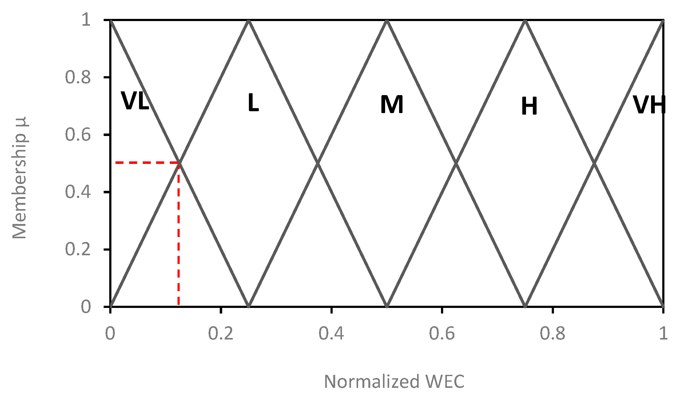
The proposed benchmarking method with both aspects, the spatial and temporal benchmarking approaches, are shown to illustrate how these two types of benchmarking systems can address the uncertainties and their ability to underpin underlying causes that affect HEIs performance. To improve on benchmarking and communicating performance. Twenty-one temporal scenarios are proposed to cover a wide range of judgments in human perception. Which can give a better understanding of the individual underperformer and the set of themes (i.e., climatic factors) that highly affect the university performance. 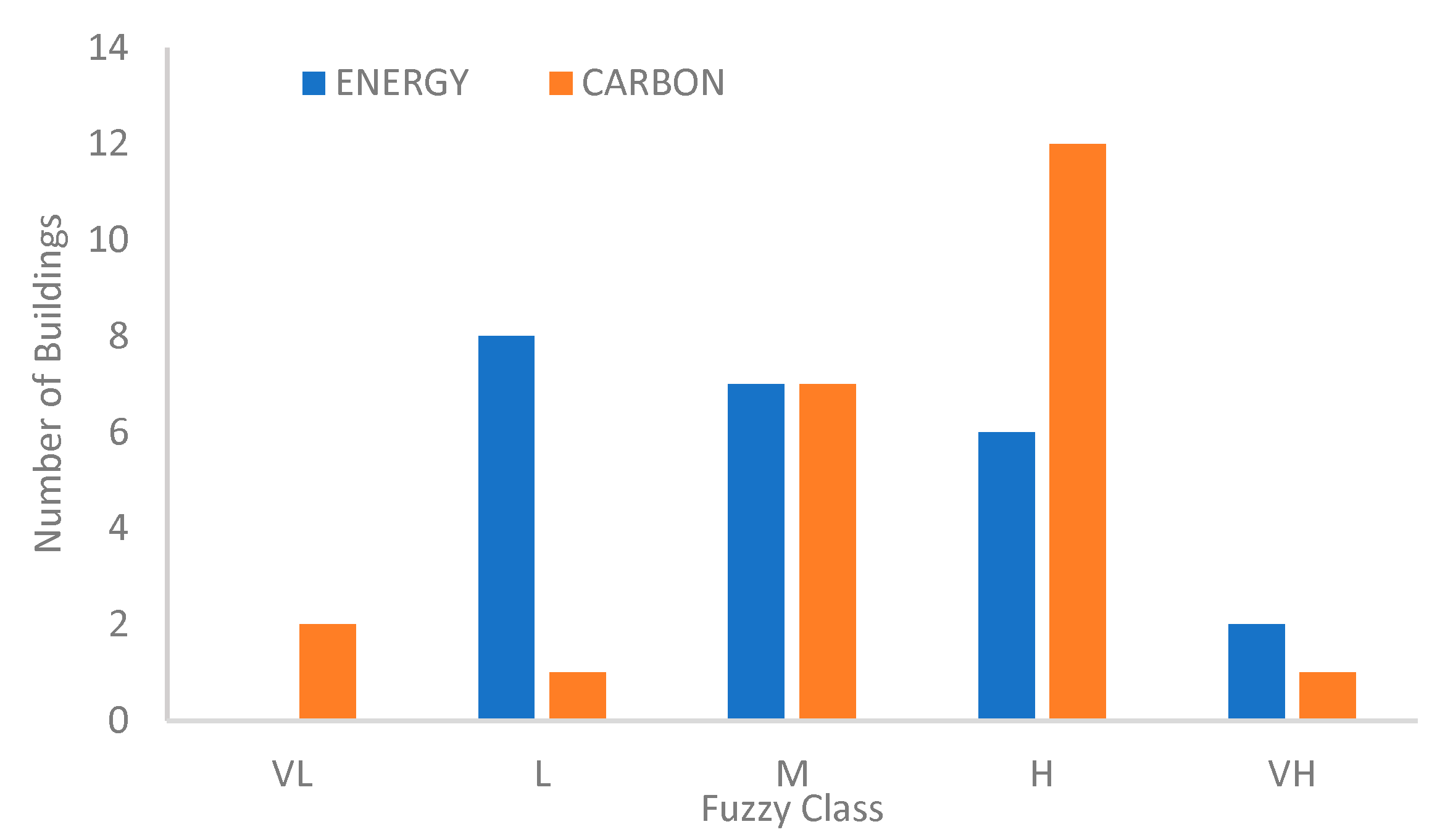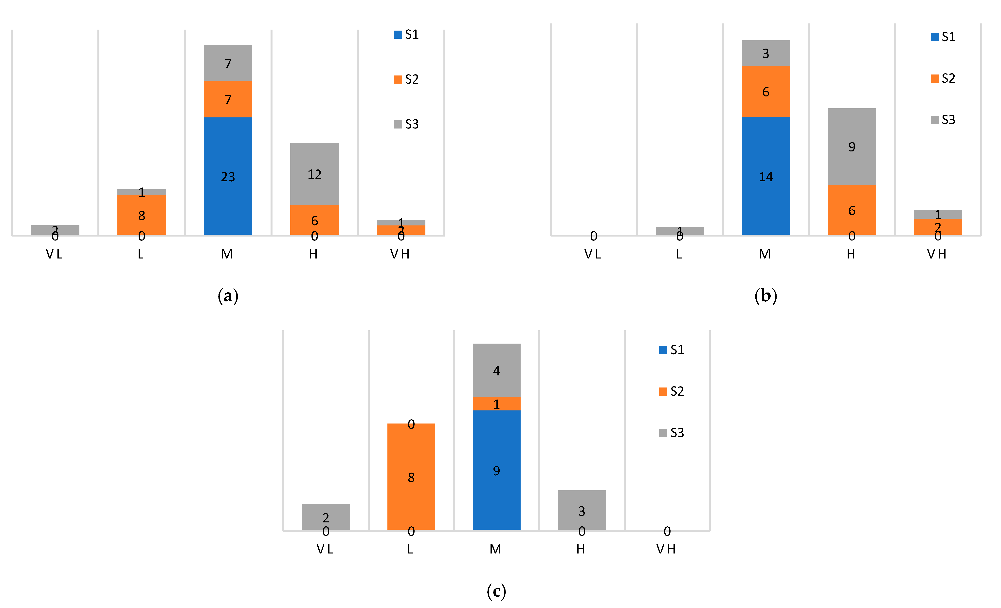Figure 12a–c shows the classification of each building by type in terms of the five classes. It can be noted that academic buildings hold a larger effect on the overall performance within the university compared to residential buildings.

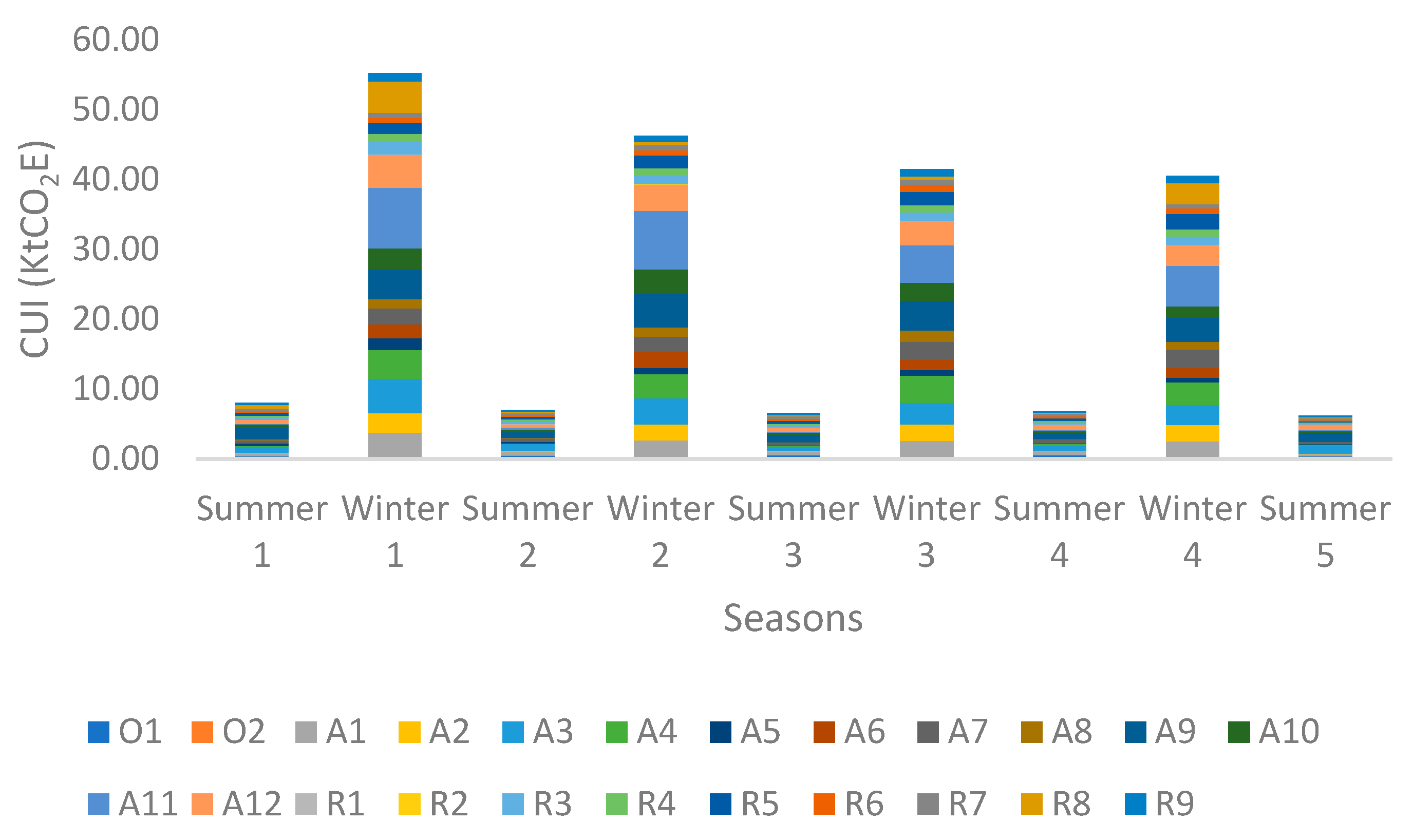
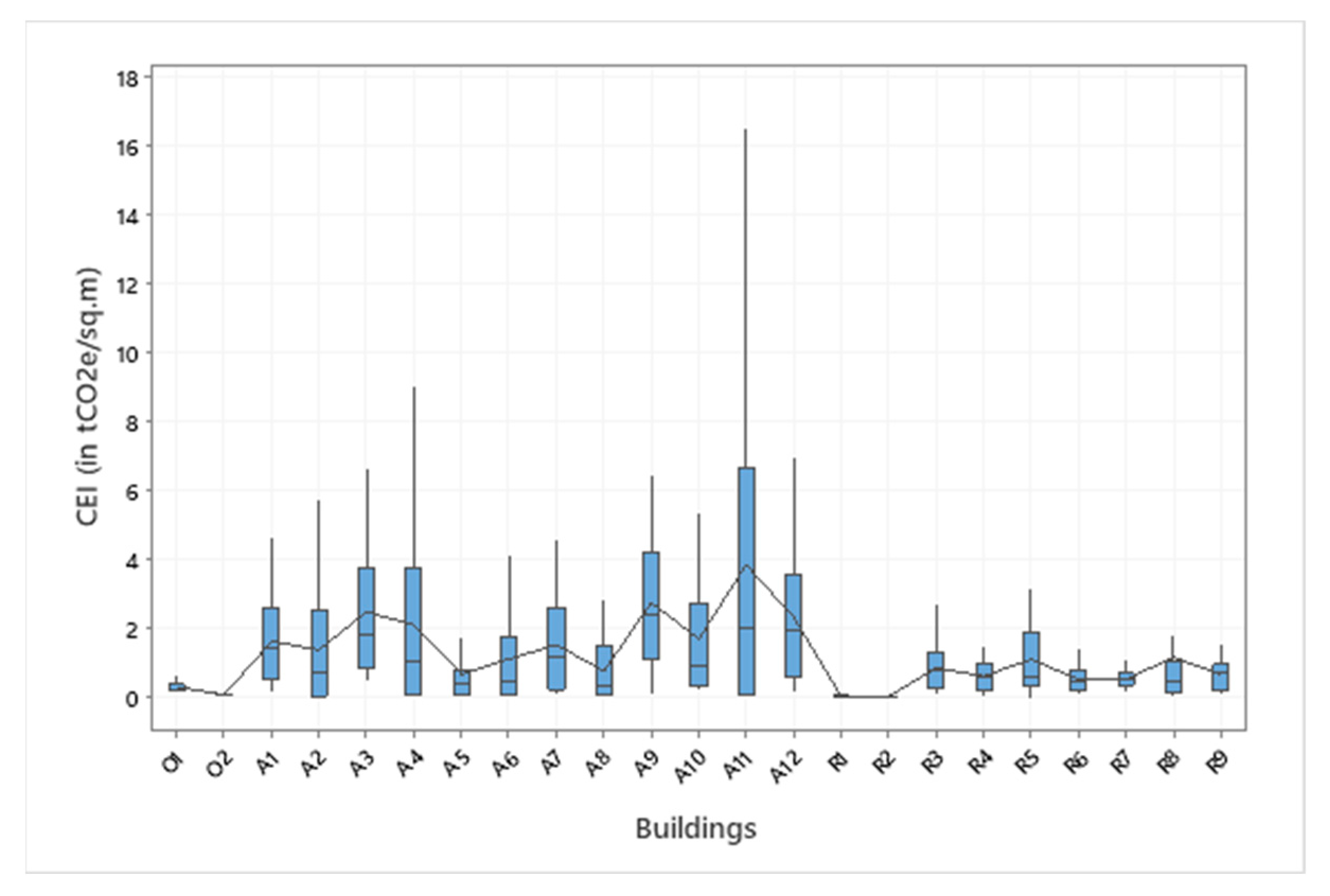
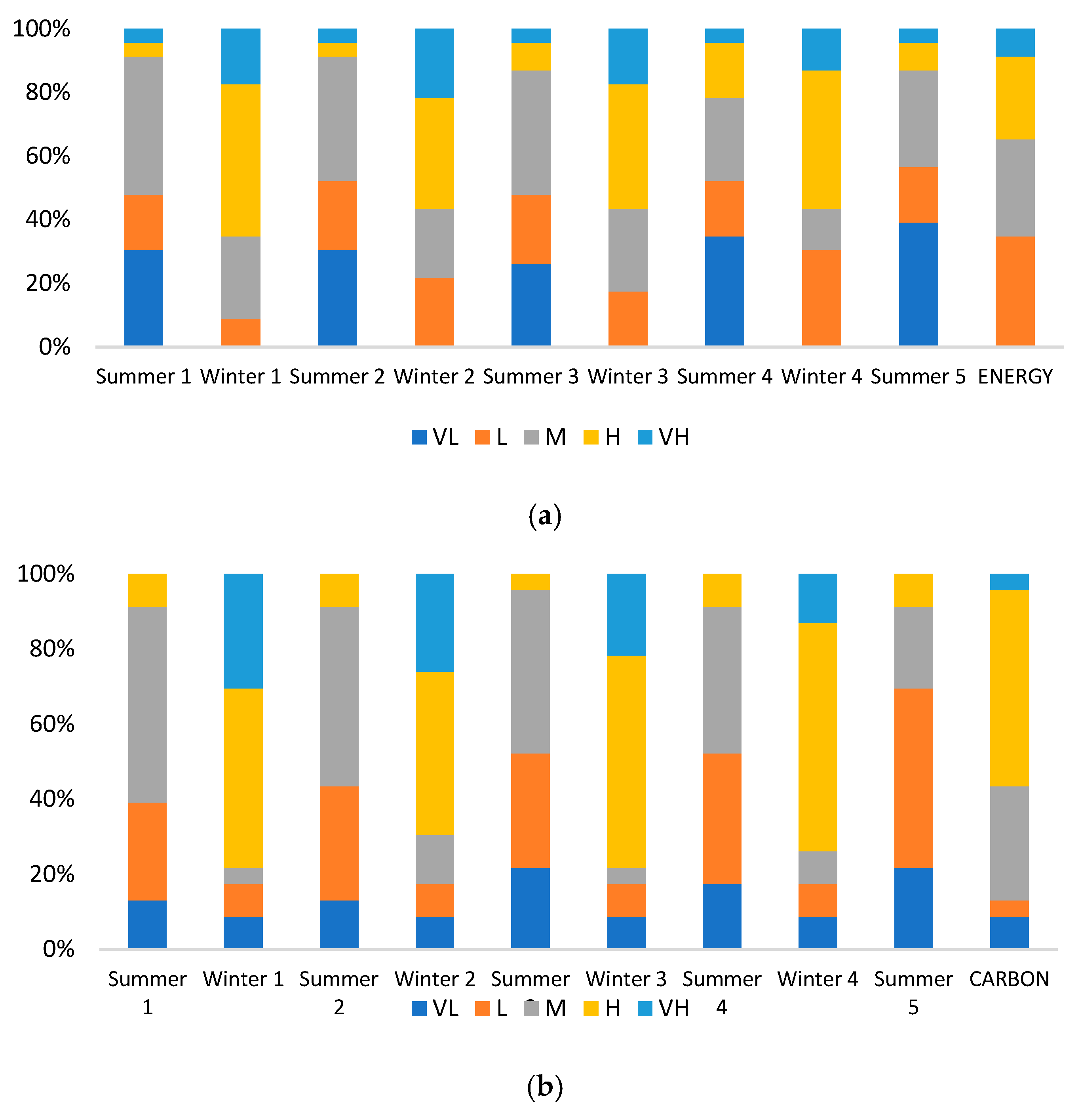
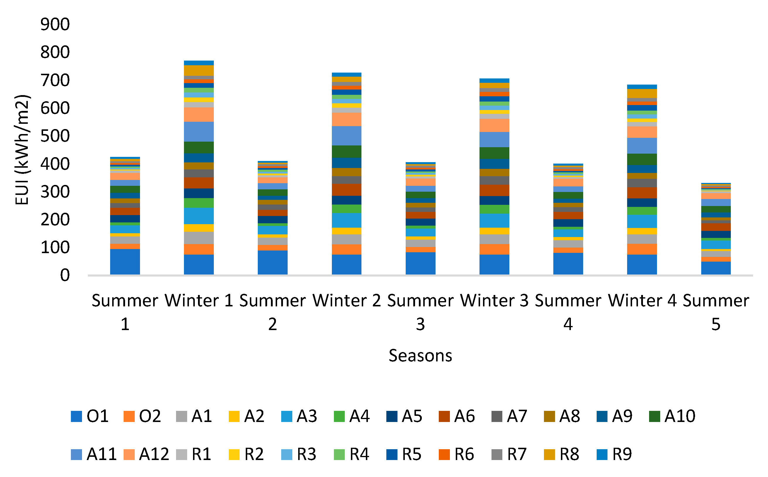
By classifying the buildings in terms of the type of buildings (i.e., academic or residential), academic (which include operational buildings), and residential buildings as a separate class. It is noted that in academic buildings in Scenario 2, 43% of the buildings fall in the (VL, L, M) class, and 57% fall in the (H, VH) class. Similarly, for Scenario 3, 29% of the academic buildings are in the (VL, L, M) class, and 71% are falling behind in the carbon scenario. Residential buildings are less impactful, since all the residential buildings fall in the (VL, L, M) class with 0 buildings in the VL class, eight buildings in the L class, and one building in the M class. In the third scenario, 67% of residential buildings are better performers, and 33% have a considerable impact on the carbon scenario. In the energy preference scenario, two buildings are noted to have VH, which are an operational building and an academic building. These two buildings have high EUI, where O1 monthly average EUI is 77.17 kWh/m² and A11 reports 44.85 kWh/m². Building A11 is reporting a VH class in both scenarios, which means this building is among the least performers in terms of energy and carbon scenarios.

This paper shows that heating requirements may be the main contributor to the energy and carbon impacts. Addressing these high-intensity areas in the buildings is a challenge for universities seeking to minimize their impact on the environment. Finally, this paper illustrated a proposal to the calculation method, based on system dynamic modeling of water–energy–carbon nexus and the carbon sequestration in HEIs. It also showed that, due to the intensive nature of academic buildings, biological sequestration may not be a viable option for universities to pursue—especially in regions where water resources are heavily dependent on fossil fuels.

References

1. Hernandez, P.; Burke, K.; Lewis, J.O. Development of energy performance benchmarks and building energy ratings for non-domestic buildings: An example for Irish primary schools. Energy Build. 2008, 40, 249–254. [Google Scholar] [CrossRef]
2. Hong, S.; Mylona, A.; Davies, H.; Ruyssevelt, P.; Mumovic, D. Assessing the trends of energy use of public non-domestic buildings in England and Wales. Build. Serv. Eng. Res. Technol. 2018, 40, 176–197. [Google Scholar] [CrossRef]
3. EPA. Users Guide to the 2012 CBECS Large Buildings Water Usage Public Use Microdata File; EPA: Washington, DC, USA, 2017.
4. Zhang, J. UC Berkeley Water Usage & Conservation Study Report; University of California: Berkeley, CA, USA, 2010. [Google Scholar]
5. Alghamdi, A.; Hu, G.; Haider, H.; Hewage, K.; Sadiq, R. Benchmarking of Water, Energy, and Carbon Flows in Academic Buildings: A Fuzzy Clustering Approach. Sustainability 2020, 12, 4422. [Google Scholar] [CrossRef]
6. Meda, A.; Lensch, D.; Schaum, C.; Cornel, P.; Lazarova, V.; Choo, K. Energy and water: Relations and recovery potential. In Water-Energy Interactions in Water Reuse; IWA Publishing: London, UK, 2012; pp. 21–35. ISBN 9781843395416. [Google Scholar]
7. Van Dijk, M.P.; Mingshun, Z. Sustainability indices as a tool for urban managers, evidence from four medium-sized Chinese cities. Environ. Impact Assess. Rev. 2005, 25, 667–688. [Google Scholar] [CrossRef]
8. Gasparatos, A.; El-Haram, M.; Horner, M. A critical review of reductionist approaches for assessing the progress towards sustainability. Environ. Impact Assess. Rev. 2008, 28, 286–311. [Google Scholar] [CrossRef]
9. Nardo, M.; Saisana, M.; Saltelli, A.; Tarantola, S.; Hoffman, A.; Giovannini, E. Handbook on Constructing Composite Indicators: Methodology and User Guide; OCED: Paris, France, 2005. [Google Scholar]
10. Agdas, D.; Srinivasan, R.S.; Frost, K.; Masters, F.J. Energy use assessment of educational buildings: Toward a campus-wide sustainable energy policy. Sustain. Cities Soc. 2015, 17, 15–21. [Google Scholar] [CrossRef] [Green Version]
11. Gasparatos, A.; Scolobig, A. Choosing the most appropriate sustainability assessment tool. Ecol. Econ. 2012, 80, 1–7. [Google Scholar] [CrossRef]
12. Hu, G.; Bakhtavar, E.; Hewage, K.; Mohseni, M.; Sadiq, R. Heavy metals risk assessment in drinking water: An integrated probabilistic-fuzzy approach. J. Environ. Manag. 2019, 250, 109514. [Google Scholar] [CrossRef] [PubMed]
13. Darbra, R.M.; Eljarrat, E.; Barceló, D. How to measure uncertainties in environmental risk assessment. Trac Trends Anal. Chem. 2008, 27, 377–385. [Google Scholar] [CrossRef] [Green Version]
14. Haider, H.; Hewage, K.; Umer, A.; Ruparathna, R.; Chhipi-Shrestha, G.; Culver, K.; Holland, M.; Kay, J.; Sadiq, R. Sustainability assessment framework for small-sized urban neighbourhoods: An application of fuzzy synthetic evaluation. Sustain. Cities Soc. 2018, 36, 21–32. [Google Scholar] [CrossRef]
15. AASHE. STARS Technical Manual Version 2.1. Available online: http://www.aashe.org/files/documents/STARS/2.0/stars_2.1_technical_manual_-_administrative_update_two.pdf (accessed on 4 November 2017).
16. Khoshbakht, M.; Gou, Z.; Dupre, K. Energy use characteristics and benchmarking for higher education buildings. Energy Build. 2018, 164, 61–76. [Google Scholar] [CrossRef] [Green Version]
17. Nunayon, S.S.; Olanipekun, E.A.; Famakin, I.O. Determining key drivers of efficient electricity management practices in public universities in Southwestern Nigeria. Int. J. Sustain. High. Educ. 2020, 21, 281–314. [Google Scholar] [CrossRef]
18. Alghamdi, A.; Haider, H.; Hewage, K.; Sadiq, R. Inter-University Sustainability Benchmarking for Canadian Higher Education Institutions: Water, Energy, and Carbon Flows for Technical-Level Decision-Making. Sustainability 2019, 11, 2599. [Google Scholar] [CrossRef] [Green Version]
19. Santamouris, M.; Mihalakakou, G.; Patargias, P.; Gaitani, N.; Sfakianaki, K.; Papaglastra, M.; Pavlou, C.; Doukas, P.; Primikiri, E.; Geros, V.; et al. Using intelligent clustering techniques to classify the energy performance of school buildings. Energy Build. 2007, 39, 45–51. [Google Scholar] [CrossRef]
20. Chung, W.; Hui, Y.V.; Lam, Y.M. Benchmarking the energy efficiency of commercial buildings. Appl. Energy 2006, 83, 1–14. [Google Scholar] [CrossRef]
21. Sadiq, R.; Rodriguez, M.J. Fuzzy synthetic evaluation of disinfection by-products—A risk-based indexing system. J. Environ. Manag. 2004, 73, 1–13. [Google Scholar] [CrossRef] [Green Version]
22. Khan, F.I.; Sadiq, R. Risk-Based Prioritization of Air Pollution Monitoring Using Fuzzy Synthetic Evaluation Technique. Environ. Monit. Assess. 2005, 105, 261–283. [Google Scholar] [CrossRef] [PubMed] [Green Version]
23. Kaivo-oja, J.R.L.; Lauraeus, I.T. The VUCA approach as a solution concept to corporate foresight challenges and global technological disruption. Foresight 2018, 20, 27–49. [Google Scholar] [CrossRef]
24. IPCC. Climate Change 2014: Mitigration of Climate Change; Cambridge University Press: Cambridge, UK, 2014. [Google Scholar]
25. Smith, C.J.; Forster, P.M.; Allen, M.; Fuglestvedt, J.; Millar, R.J.; Rogelj, J.; Zickfeld, K. Current fossil fuel infrastructure does not yet commit us to 1.5 °C warming. Nat. Commun. 2019, 10, 101. [Google Scholar] [CrossRef] [Green Version]
26. Den Elzen, M.; Admiraal, A.; Roelfsema, M.; van Soest, H.; Hof, A.F.; Forsell, N. Contribution of the G20 economies to the global impact of the Paris agreement climate proposals. Clim. Change 2016, 137, 655–665. [Google Scholar] [CrossRef] [Green Version]
27. Wang, X.-C.; Klemeš, J.J.; Ouyang, X.; Xu, Z.; Fan, W.; Wei, H.; Song, W. Regional Embodied Water-Energy-Carbon Efficiency of China. Energy 2021, 224, 120159. [Google Scholar] [CrossRef]
28. Liu, X.; Klemeš, J.J.; Varbanov, P.S.; Čuček, L.; Qian, Y. Virtual carbon and water flows embodied in international trade: A review on consumption-based analysis. J. Clean. Prod. 2017, 146, 20–28. [Google Scholar] [CrossRef]
29. IEA. CO2 Emissions from Fuel Combustion: Annual Time Series of CO2 Emissions from Fossil Fuel Combustion a Major Source of Anthropogenic Greenhouse Gas Emissions. Available online: https://www.iea.org/data-and-statistics/data-product/co2-emissions-from-fuel-combustion (accessed on 4 May 2021).
30. DOE. Chapter 5: Increasing efficiency of building systems and technologies. In Quadrennial Technology Review: An Assessment of Energy Technologies and Research Opportunities; DOE: Washington, DC, USA, 2015. [Google Scholar]
31. Asimakopoulos, D.A.; Santamouris, M.; Farrou, I.; Laskari, M.; Saliari, M.; Zanis, G.; Giannakidis, G.; Tigas, K.; Kapsomenakis, J.; Douvis, C.; et al. Modelling the energy demand projection of the building sector in Greece in the 21st century. Energy Build. 2012, 49, 488–498. [Google Scholar] [CrossRef]
32. Zhang, A.; Bokel, R.; Van den Dobbelsteen, A.; Sun, Y.; Huang, Q.; Zhang, Q. The Effect of Geometry Parameters on Energy and Thermal Performance of School Buildings in Cold Climates of China. Sustainability 2017, 9, 1708. [Google Scholar] [CrossRef] [Green Version]
33. Papadopoulos, S.; Kontokosta, C.E. Grading buildings on energy performance using city benchmarking data. Appl. Energy 2019, 233–234, 244–253. [Google Scholar] [CrossRef]
34. Gul, M.S.; Patidar, S. Understanding the energy consumption and occupancy of a multi-purpose academic building. Energy Build. 2015, 87, 155–165. [Google Scholar] [CrossRef] [Green Version]
35. Canada, E. Pan-Canadian Framework on Clean Growth and Climate Change: Canada’s Plan to Address Climate Change and Grow the Economy; Environment and Climate Change Canada: Gatineau, QC, Canada, 2016. Available online: http://publications.gc.ca/site/eng/9.828774/publication.html (accessed on 24 October 2020).
36. Scheuer, C.; Keoleian, G.A.; Reppe, P. Life cycle energy and environmental performance of a new university building: Modeling challenges and design implications. Energy Build. 2003, 35, 1049–1064. [Google Scholar] [CrossRef]
37. NRC. Energy Efficiency Trends in Canada 1990–2010; National Research Council Canada: Ottawa, ON, Canada, 2013; pp. 1926–8254.
38. Chung, M.H.; Rhee, E.K. Potential opportunities for energy conservation in existing buildings on university campus: A field survey in Korea. Energy Build. 2014, 78, 176–182. [Google Scholar] [CrossRef]
39. Brown, M.A.; Southworth, F. Mitigating Climate Change through Green Buildings and Smart Growth. Environ. Plan. Econ. Space 2008, 40, 653–675. [Google Scholar] [CrossRef] [Green Version]
40. Faulconbridge, J. Mobil ‘gree’ design knowledge: Institutions, bricolage and the relational production of embedded sustainable building design. Trans. Inst. Br. Geogr. 2013, 38, 339–353. [Google Scholar] [CrossRef] [Green Version]
41. Mahmoodzadeh, M.; Gretka, V.; Blue, A.; Adams, D.; Dallimore, B.; Mukhopadhyaya, P. Evaluating Thermal Performance of Vertical Building Envelopes: Case Studies in a Canadian University Campus. J. Build. Eng. 2021, 40, 102712. [Google Scholar] [CrossRef]
42. NRC. Consumption of Energy Survey for Universities, Colleges and Hospitals 2003. Available online: http://oee.nrcan.gc.ca/corporate/statistics/neud/dpa/data_e/consumption03/universities.cfm?attr=0 (accessed on 18 November 2020).
43. Tan, H.; Chen, S.; Shi, Q.; Wang, L. Development of green campus in China. J. Clean. Prod. 2014, 64, 646–653. [Google Scholar] [CrossRef]
44. ENERGYSTAR. Facility Type: K-12 Schools; 2006. Available online: https://www.energystar.gov/sites/default/files/buildings/tools/EPA_BUM_CH10_Schools.pdf (accessed on 10 October 2017).
45. Gyan, C.-S.; Kasun, H.; Rehan, S. Water–Energy–Carbon Nexus Modeling for Urban Water Systems: System Dynamics Approach. J. Water Resour. Plan. Manag. 2017, 143, 04017016. [Google Scholar] [CrossRef]
46. Alshuwaikhat, H.M.; Abubakar, I. An integrated approach to achieving campus sustainability: Assessment of the current campus environmental management practices. J. Clean. Prod. 2008, 16, 1777–1785. [Google Scholar] [CrossRef] [Green Version]
47. Geng, Y.; Liu, K.; Xue, B.; Fujita, T. Creating a “green university” in China: A case of Shenyang University. J. Clean. Prod. 2013, 61, 13–19. [Google Scholar] [CrossRef]
48. Ministy of Environment BC. Carbon Neutral Government Year in Review 2018: Summary. 2018. Available online: https://www2.gov.bc.ca/assets/gov/environment/climate-change/cnar/2018/347953_attachment_cng_annual_report_summary_2018.pdf (accessed on 11 January 2020).
49. EPA. Educational Facilities. 2012. Available online: https://www.epa.gov/watersense/types-facilities (accessed on 7 December 2019).
50. Ward, I.; Ogbonna, A.; Altan, H. Sector review of UK higher education energy consumption. Energy Policy 2008, 36, 2939–2949. [Google Scholar] [CrossRef]
51. Li, X.; Tan, H.; Rackes, A. Carbon footprint analysis of student behavior for a sustainable university campus in China. J. Clean. Prod. 2015, 106, 97–108. [Google Scholar] [CrossRef]
52. Chihib, M.; Salmerón-Manzano, E.; Manzano-Agugliaro, F. Benchmarking Energy Use at University of Almeria (Spain). Sustainability 2020, 12, 1336. [Google Scholar] [CrossRef] [Green Version]
53. Alghamdi, N.; den Heijer, A.; de Jonge, H. Assessment tools’ indicators for sustainability in universities: An analytical overview. Int. J. Sustain. High. Educ. 2017, 18, 84–115. [Google Scholar] [CrossRef]
54. Wichowski, P.P.; Rutkowska, G.; Kamiński, N.; Trach, Y. Analysis of Water Consumption in the Campus of Warsaw University of Life Sciences—SGGW in Years 2012–2016. J. Ecol. Eng. 2019, 20, 193–202. [Google Scholar] [CrossRef]
55. Hu, M. Life-cycle environmental assessment of energy-retrofit strategies on a campus scale. Build. Res. Inf. 2020, 48, 659–680. [Google Scholar] [CrossRef]
56. Misni, A.; Buyadi, S.N.A.; Kamaruddin, S.M.; Ahmad, P. Quantifying Carbon Footprint Review in University Campus. Environ. Behav. Proc. J. 2019, 4, 131–138. [Google Scholar] [CrossRef] [Green Version]
57. Bernardo, H.; Oliveira, F. Estimation of Energy Savings Potential in Higher Education Buildings Supported by Energy Performance Benchmarking: A Case Study. Environments 2018, 5, 85. [Google Scholar] [CrossRef] [Green Version]
58. Larsen, H.N.; Pettersen, J.; Solli, C.; Hertwich, E.G. Investigating the Carbon Footprint of a University—The case of NTNU. J. Clean. Prod. 2013, 48, 39–47. [Google Scholar] [CrossRef]
59. Ramsden, B. Patterns of Higher Education Institutions in the UK: Seventh Report; University of London: London, UK, 2007. [Google Scholar]
60. Davis, J.A.; Nutter, D.W. Occupancy diversity factors for common university building types. Energy Build. 2010, 42, 1543–1551. [Google Scholar] [CrossRef]
61. Sharp, T.R. Benchmarking energy use in schools. In Proceedings of the ACEEE 1998 Summer Study on Energy Efficiency in Buildings, Washington, DC, USA, 1 October 1998; Volume 3, pp. 3305–3316. [Google Scholar]
62. Gallachóir, B.Ó.; Keane, M.; Morrissey, E.; O’Donnell, J. Using indicators to profile energy consumption and to inform energy policy in a university—A case study in Ireland. Energy Build. 2007, 39, 913–922. [Google Scholar] [CrossRef]
63. Mazzarella, L. Energy retrofit of historic and existing buildings. The legislative and regulatory point of view. Energy Build. 2015, 95, 23–31. [Google Scholar] [CrossRef]
64. Caeiro, S.; Filho, W.L.; Jabbour, C.; Azeiteiro, U.M. Sustainability Assessment Tools in Higher Education Institutions; Springer International Publishing: Berlin/Heidelberg, Germany, 2013; p. 432. [Google Scholar] [CrossRef]
65. Juodis, E.; Jaraminiene, E.; Dudkiewicz, E. Inherent variability of heat consumption in residential buildings. Energy Build. 2009, 41, 1188–1194. [Google Scholar] [CrossRef]
66. Hartungi, R.; Jiang, L. Energy efficiency and conservation in an office building: A case study. Int. J. Energy Sect. Manag. 2012, 6, 175–188. [Google Scholar] [CrossRef]
67. Zirkle, G.; Lal, R.; Augustin, B.; Follett, R. Modeling Carbon Sequestration in the U.S. Residential Landscape. In Carbon Sequestration in Urban Ecosystems; Lal, R., Augustin, B., Eds.; Springer: Dordrecht, The Netherlands, 2012; pp. 265–276. [Google Scholar] [CrossRef]
68. Bass, S.; Dalal-Clayton, B. Sustainable Development Strategies: A Resource Book/Compiled by Barry Dalal-Clayton and Stephen Bass; Routledge: London, UK, 2002.
69. WCED. Our Common Future: The World Commission on Environment and Development; United Nations Environmental Program Oxford University Press: Oxford, UK, 1987; p. 300. [Google Scholar]
70. Martin, S.; Jucker, R. Educating Earth-literate Leaders. J. Geogr. High. Educ. 2005, 29, 19–29. [Google Scholar] [CrossRef]
71. UBCO. Campus Facts 2019; The University of British Columbia Okanagan: Kelowna, BC, Canada, 2019. [Google Scholar]
72. Climatemps. Vancouver British Columbia and Kelowna BC Climate & Distance in Between. Available online: http://www.vancouver.climatemps.com/vs/kelowna.php (accessed on 18 January 2020).
73. WeatherStats. About Kelowna. Available online: https://kelowna.weatherstats.ca/about.html (accessed on 4 July 2021).
74. BEF. Calculate Your Business Water Use. Available online: https://store.b-e-f.org/calculate-business-footprint/water/#water_use (accessed on 1 March 2021).
75. Chhipi Shrestha, G.K. Water-Energy-Carbon Nexus: A System Dynamics Approach for Assessing Urban Water Systems. Doctoral Dissertation, University of British Columbia, Vancouver, BC, Canada, 2017. [Google Scholar]
76. OBWB. Agriculture Water Demand Model; Okanagan Basin Water Board: Kelowna, BC, Canada, 2010. [Google Scholar]
77. British Columbia Ministry of Environment. 2016/2017 B.C. Best Practices Methodology for Quanitifying Greenhouse Gas Emissions; Ministry of Environment: Victoria, BC, Canada, 2016.
78. Chhipi-Shrestha, G.; Hewage, K.; Sadiq, R. Impacts of neighborhood densification on water-energy-carbon nexus: Investigating water distribution and residential landscaping system. J. Clean. Prod. 2017, 156, 786–795. [Google Scholar] [CrossRef]
79. Uricchio, V.F.; Giordano, R.; Lopez, N. A fuzzy knowledge-based decision support system for groundwater pollution risk evaluation. J. Environ. Manag. 2004, 73, 189–197. [Google Scholar] [CrossRef]
80. Schuhmacher, M.; Meneses, M.; Xifró, A.; Domingo, J.L. The use of Monte-Carlo simulation techniques for risk assessment: Study of a municipal waste incinerator. Chemosphere 2001, 43, 787–799. [Google Scholar] [CrossRef]
81. Hu, G.; Kaur, M.; Hewage, K.; Sadiq, R. An integrated chemical management methodology for hydraulic fracturing: A fuzzy-based indexing approach. J. Clean. Prod. 2018, 187, 63–75. [Google Scholar] [CrossRef]
82. Saaty, R.W. The analytic hierarchy process—What it is and how it is used. Math. Model. 1987, 9, 161–176. [Google Scholar] [CrossRef] [Green Version]
83. Saaty, T.L.; Vargas, L. Models, Methods, Concepts & Applications of the Analytic Hierarchy Process; Springer: Berlin/Heidelberg, Germany, 2012. [Google Scholar]
84. Wind, Y.; Saaty, T.L. Marketing Applications of the Analytic Hierarchy Process. Manag. Sci. 1980, 26, 641–658. [Google Scholar] [CrossRef]
85. Reza, B.; Sadiq, R.; Hewage, K. Sustainability assessment of flooring systems in the city of Tehran: An AHP-based life cycle analysis. Constr. Build. Mater. 2011, 25, 2053–2066. [Google Scholar] [CrossRef]
86. Raharjo, H.; Endah, D. Evaluating Relationship of Consistency Ratio and Number of Alternatives on Rank Reversal in the AHP. Qual. Eng. 2006, 18, 39–46. [Google Scholar] [CrossRef]
87. Lu, R.-S.; Lo, S.-L.; Hu, J.-Y. Analysis of reservoir water quality using fuzzy synthetic evaluation. Stoch. Environ. Res. Risk Assess. 1999, 13, 327–336. [Google Scholar] [CrossRef]
88. Cheng, C.-H.; Lin, Y. Evaluating the best main battle tank using fuzzy decision theory with linguistic criteria evaluation. Eur. J. Oper. Res. 2002, 142, 174–186. [Google Scholar] [CrossRef]
89. FortisBC. Public Sector Organizations: Reducing GHF emissions with RNG. Available online: https://www.fortisbc.com/services/sustainable-energy-options/renewable-natural-gas/public-sector-organizations-reducing-ghg-emissions-with-rng (accessed on 1 September 2020).
90. UBCO. Geoexchange. Available online: https://facilities.ok.ubc.ca/geoexchange/ (accessed on 21 September 2020).
91. UBCO. Carbon Neutral Action Report; UBCO-Sustainability Office: Kelowna, BC, Canada, 2019; Available online: https://sustain.ok.ubc.ca/reports/cnar/ (accessed on 27 October 2020).
92. COK. City of Kelowna Sustainable Urban Forest Strategy 2011–2021; Kelowna Municipality: Kelowna, BC, Canada, 2011. [Google Scholar]
93. PalisadeCorp. At Risk Version 8.1 Palisade Corporation; PalisadeCorp: Ithaca, NY, USA, 2021. [Google Scholar]
94. Fuller, R. On Obtaining OWA Operator Weights: A Sort Survey of Recent Developments. In Proceedings of the 2007 IEEE International Conference on Computational Cybernetics, Gammarth, Tunisia, 19–21 October 2007; pp. 241–244. [Google Scholar]
Figure 1. Probabilistic fuzzy synthetic framework.
Environments 08 00072 g001
Figure 2. Fuzzification and fuzzy memberships.
Environments 08 00072 g002
Figure 3. AHP hierarchy structure.
Environments 08 00072 g003
Figure 4. The trend of water consumption.
Environments 08 00072 g004
Figure 5. Ratio-to-area and BEF box-plot.
Environments 08 00072 g005
Figure 6. Box-plots of EUIs calculated for different buildings on campus.
Environments 08 00072 g006
Figure 7. Historic GHG emissions in the campus.
Environments 08 00072 g007
Figure 8. Box-plot of the calculated CUI in the university.
Environments 08 00072 g008
Figure 9. Water–energy–carbon nexus of the supplied water at campus (a) water quantity, (b) energy from water usage, (c) carbon emission from the energy needed to use water at the campus level, and its corresponding energy use.
Environments 08 00072 g009
Figure 10. Temporal preference scenarios: (a) Energy, (b) carbon.
Environments 08 00072 g010
Figure 11. Energy and carbon preference scenarios classification per building.
Environments 08 00072 g011
Figure 12. Results of scenario analysis, (a) buildings per proposed class, (b) academic buildings per class, and (c) residential buildings per class.
Environments 08 00072 g012