Convolutional Neural Network-Based Gear Type Identification from Automatic Identification System Trajectory Data

Abstract

Marine resources are valuable assets to be protected from illegal, unreported, and unregulated (IUU) fishing and overfishing. IUU and overfishing detections require the identification of fishing gears for the fishing ships in operation. This paper is concerned with automatically identifying fishing gears from AIS (automatic identification system)-based trajectory data of fishing ships. It proposes a deep learning-based fishing gear-type identification method in which the six fishing gear type groups are identified from AIS-based ship movement data and environmental data. The proposed method conducts preprocessing to handle different lengths of messaging intervals, missing messages, and contaminated messages for the trajectory data. For capturing complicated dynamic patterns in trajectories of fishing gear types, a sliding window-based data slicing method is used to generate the training data set. The proposed method uses a CNN (convolutional neural network)-based deep neural network model which consists of the feature extraction module and the prediction module. The feature extraction module contains two CNN submodules followed by a fully connected network. The prediction module is a fully connected network which suggests a putative fishing gear type for the features extracted by the feature extraction module from input trajectory data. The proposed CNN-based model has been trained and tested with a real trajectory data set of 1380 fishing ships collected over a year. A new performance index, DPI (total performance of the day-wise performance index) is proposed to compare the performance of gear type identification techniques. To compare the performance of the proposed model, SVM (support vector machine)-based models have been also developed. In the experiments, the trained CNN-based model showed 0.963 DPI, while the SVM models showed 0.814 DPI on average for the 24-h window. The high value of the DPI index indicates that the trained model is good at identifying the types of fishing gears.

1. Introduction

Almost 37% of the global population depends on fish and fish products for their protein intake [1]. Global warming and exponential population growth have largely reduced the food supply from marine environments, and there are concerns about the sustainability of proteins obtained from these marine environments. According to FAO [2], the fishing industry has faced various challenges such as fish stock preservation from overfishing and biodiversity loss and financial sustainability management from profit reduction due to depletion of fish resources. Illegal, unreported, and unregulated (IUU) fishing and overfishing are severe threats to the sustainability of marine ecosystems and fish stock preservation [3,4,5]. IUU fishing may cause fishing stock collapse and is not economically viable.

Two important IUU fishing types are fishing in areas that have been designated as no-fishing water areas and fishing with unpermitted fishing gears. It is relatively easy for fishery monitoring officers to determine whether a fishing ship is fishing in a no-fishing water area based on its location and speed [6]. In Korea, each fishing ship has its fishing gear license, which is officially registered into the Korean Fishing Ship Register Database [7]. It is illegal for a fishing ship to use some unlicensed fishing gears. Even though a fishery monitoring officer knows the location, speed, and course of a fishing ship in real-time, it is difficult to identify the type of fishing gear being used because fishing ships with a specific type of fishing gear may show many variations in movement trajectories and such identification requires examination of a long trajectory over upwards of 24 h. Hence it is crucial to identify the types of fishing gear used on fishing ships from the available monitoring data for the prevention of IUU fishing. Fishing gear type identification allows to estimate fishing type and fish catch and further helps to detect IUU fishing. Hence such activities are valuable for preserving marine resources and preventing from overfishing. A computerized automatic fishing type identification system with the fishing ship register database can monitor fishing activities in the surveillance regions and detect IUU fishing activities with no risks of collusion between fishers and inspectors [8,9].

Fishing ships are usually equipped with a VMS (vessel monitoring system)-based communication device, which sends voice and digital messages through a satellite or MF/HF communication channel [10]. As in European countries, Korea has established VHF-DSC and satellite-based VMS system for fishery monitoring in accordance with the FAO guideline for IUU prevention.

A VMS device automatically sends status data such as location, speed, and course to fishery monitoring agencies at long intervals such as 1 h or 2 h [11,12]. There has been some work focused on using VMS data for the identification of fishing activities such as fishing/non-fishing or setting/hauling/others [13,14,15,16,17,18]. It is, however, inappropriate to use VMS data for fishing gear type identification because the sparsely available data on ship movement does not provide sufficient information.

In accordance with the IMO’s (International Maritime Organization) regulations for navigation safety, it is mandatory for fishing ships of minimum length 10 m to be equipped with an AIS (automatic identification system) device which broadcasts messages about location and course at intervals of 2 to 12 s. Most countries including Korea enforce fishing ships to be equipped with AIS devices.

Such fine-resolution AIS messages contain information for recovering accurate ship trajectories. Hence AIS data are more advantageous than VMS data for fishing gear-type identification. On the other hand, the movements of fish schools are affected by environmental factors such as water temperature, pH, dissolved oxygen, and food availability (like micro-plankton). Such environmental data are helpful for fishing gear-type identification of fishing ships.

This paper presents a deep-learning based method for fishing gear-type identification which uses both AIS data and marine environmental data. It introduces a preprocessing method for AIS data to handle different messaging intervals, missing messages, and contaminated messages. It uses a sliding window-based data slicing method to capture complicated dynamic patterns over trajectories depending on the fishing gear type. The developed deep-learning based method uses two 1D CNN (one dimensional convolutional neural network) submodules and a fully connected network module for feature extraction and a fully connected network-based prediction module which suggests a promising fishing gear type from the input trajectory data. The trained model classifies the fishing works into six fishing gear types, i.e., purse seine, stow net, longline, drift gill nets, traps, and trawl. The model has been trained and tested using real trajectory data of 1380 fishing ships over the one year. It presents a new performance index, DPI, which stands for total performance of day-wise performance index. In the experiments, the trained model showed a 0.963 DPI value for a 24-h window. The high value of the DPI index indicates that the trained model is good at identifying fishing gear types.

The remainder of this paper is organized as follows. Section 2 presents some work related to ship activity identification. Section 3 describes how to preprocess AIS data and label the training and testing data and how to prepare the training data and organize a deep-learning model for activity identification. Section 4 shows some experimental results of the proposed method. Finally, Section 5 draws conclusions from the previously presented information.

2. Related Work

Most fishing activity identification methods have been developed for VMS data. VMS data allows for proper monitoring of the movements of fishing ships with a temporal resolution of hourly order. VMS data are useful for the estimation of fishing effort, which is fundamental data for inventory management in fisheries [13]. Fishing ships broadcast messages containing their unique identifier, like a maritime mobile service identities (MMSI) number, with which their associated information like fishing gear type can be retrieved from the vessel register (VR) database. To identify the fishing activities, such as fishing or non-fishing and setting or hauling, the VMS data analysis methods interpolate the trajectories of fishing ships over a long period of time (e.g., 30 days). The methods discriminate fishing activities from the interpolated trajectories data by exploiting the information on fishing gear type retrieved from the VR database.

There have been some works that have focused on determining whether a fishing ship of a specific type is engaging in a fishing activity or on a non-fishing activity from the speed profile information extracted from the interpolated trajectory data. Marzuki proposed a method to identify the three fishing activities such as setting, hauling, and others (streaming, soak-time) for longliners [14]. He conducted the statistical analysis fishing ship speed for each fishing activity, and found out the speed ranges of each activity as follows: setting (4–6 knots), hauling (2–4 knots), and others (less than 2 knots or greater than 6 knots). His method is only applicable to a specific fishing gear type (i.e., longliners) and his results cannot be directly applied to other fishing gear types. In addition, there are no guarantees that other fishing gear types have such simple speed profiles for activity discrimination. Piet et al. [15] used VMS data to extract information on the fishing ship fleet at three levels. The first-level analysis is conducted to determine the number of fishing ships in a fleet. The second-level analysis is made to estimate the fishing effort of fishing ships, and the third-level analysis is conducted to estimate such fishing parameters as the proportion of time spent fishing, fish speed, or gear characteristics like specific gear size.

Vermard et al. [16] proposed a Bayesian hierarchical model-based method using a hidden Markov process to identify three fishing activities (i.e., steaming, fishing, or stopping) for pelagic trawlers. Their hidden Markov model (HMM) defines the observed positions conditioned on the latent variables of fishing ship activities and movement parameters which are modeled by a Bayesian model. Their method uses the amount of time spent in the fishing state to estimate the fishing effort of a pelagic trawler from the VMS data. Joo et al. [17] proposed a hidden semi-Markov model (HSMM) to discriminate three fishing activities (i.e., searching, fishing, or cruising) from VMS data of purse-seiners used for anchovy fishing. They claimed that their HSMM model outperformed the HMM model and as well as other classification methods like support vector machine, random forest, and artificial neural network with one hidden layer. Emilly et al. [18] proposed a probabilistic state-space model to discriminate three fishing activities (i.e., fishing, stopping, or cruising) from the VMS data of tuna purse-seiners.

Russo et al. [19] proposed a neural network model which classifies the fishing work into three fishing gear types of passive gears, towed gears, and mobile gears. The method uses coarsely-grained VMS data which contains information about ship speed, course change, water depth statistics of water depths, trip duration, and maximum distance from the coast over an entire fishing trip duration of about two weeks. Their method achieved a 94.4% classification accuracy. However, their method takes into account only three fishing gear types and requires fishing trip data over about two weeks.

Sparse broadcasting of VMS data intrinsically requires interpolation of trajectories for future prediction of ship position, heading, and speed changes. Such interpolation unavoidably contains some errors or noises and its spatial resolution is sparse. The VMS data-based activity prediction methods usually are applicable to fishing activity identification but not applicable to the identification of the fishing gear type. That is, the VMS data-based method is effective for discriminating between fishing activities but is not effective for determining the type of fishing. Hence, it is hard to detect illegal fishing activities from VMS data. Nowadays many countries pay attention to illegal fishing monitoring and systematic analysis of fish catch. It is necessary for their maritime administrative party to keep monitor and analyze the fishing states for each fishing gear type. It is hence important to determine the fishing gear types from monitored trajectories data. This paper introduces a new deep-learning based identification of fishing gear types from ship trajectories data.

3. Fishing Gear Type Identification from Automatic Identification System Trajectory Data

3.1. Fishing Gear Type Identification

Marine fish generally make periodic or seasonal movements for favored conditions like temperature, pH, dissolved oxygen, food like micro-planktons, and spawning. For example, when there is little tidal range, croakers stay near the bottom floor because planktons sink down; when there is a large tidal range, planktons float around and croakers swim around at middle-depth water. Hence different tidal ranges might require fishing ships to use different fishing gears. Different fishing gear types have different fishing patterns in movements and timings for net setting, waiting, and net hauling [11]. Figure 1 shows the trajectories of a fishing ship on a fishing trip, depicted from the AIS data. A fishing trip is composed of non-fishing activities and fishing activities. In Figure 1, (a) streaming and (b) waiting are non-fishing activities while (c) setting and (d) hauling are fishing activities.

A fishing gear type is indicated by a fishing method requiring special gear. Offshore fishing methods include drift gill net, bottom trawl, longline, midwater longline, and purse seine, and so on. Each fishing gear type shows some unique patterns due to its setting and hauling styles. On the other hand, non-fishing activities such as steaming and waiting are included in all fishing gear types. Despite the existence of such unique patterns in fishing activities, the long sequences of mixed non-fishing and fishing activities for a fishing trip look very complicated and entangled. The complexity and irregularities of trajectories make it hard for fishery monitoring officers to determine the fishing gear types used on fishing ships from the ship trajectories.

Fishing ships send out AIS messages and such messages are collected and monitored by the fishery authority or vessel traffic service stations. If the fishing gear types of ships are identified from their AIS messages, fishery authorities can control IUU fishing activities and overfishing [20]. Here we propose a method to identify the fishing gear types of ships from their AIS message data.

3.2. Automatic Identification System and Its Messages

The AIS is an automated tracking device used by a ship to broadcast its state and display all the ships in its vicinity while at sea. The international maritime treaty SOLAS (Safety Of Life At Sea) sets minimum safety standards, in which merchant ships of more than 300 tonnage and all passenger ships are required to be equipped with an AIS transponder [21]. For safe navigation, some countries recently began requiring fishing ships of more than 10 m in length to have an AIS transponder. An AIS message consists of static, semi-static, and dynamic information. Static information indicates permanent information such as ship name, call sign, ship type, and ship specification. Voyage-related information is semi-static because it does not change over one voyage from departure port to destination port. It consists of data like freight details, ship draught, and the estimated time of arrival (ETA), and so on. Dynamic information in an AIS message indicates the situational information of a ship such as speed, heading, and GPS coordinates. Both static and semi-static information of a ship are broadcasted through AIS messages at a low rate, e.g., every 6 min. Dynamic information is broadcasted at different rates depending on a ship’s navigation status.

Table 1. Transmission rates of automatic identification system (AIS) messages with dynamic information.

Navigation Status	Ship Speed	Transmission Period
At anchor or moored	<3 knots	3 min
	>3 knots	10 s
Cruising	0–14 knots	10 s
	0–14 knots and changing course	3.3 s
	14–23 knots	6 s
	14–23 knots and changing course	2 s
	>23 knots	2 s

shows typical transmission rates of AIS messages with dynamic information.

3.3. Preprocessing of Trajectories from AIS Data

As mentioned in Section 3.2, AIS messages contain several types of information about ships and their movements and they are broadcast at different rates over very high frequency (VHF) channels. AIS messages are sometimes contaminated with noises caused by radio inferences with neighboring ships’ radio signals or geographic obstacles like islands. A shore-based AIS device can receive contaminated messages in which some AIS messages are missing, duplicated, erroneous, or delayed. To determine the fishing gear type of a fishing trip, a trajectory needs to be constructed from a sequence of such contaminated AIS messages [22]. Hence, the AIS message data are first cleaned to remove unreliable, erroneous, or meaningless data as follows. First, we remove adjacent duplicated AIS messages and AIS messages of which longitude or latitude difference from adjacent messages are larger than a pre-specified threshold. Second, we remove AIS messages of which locations are close to a harbor or in a harbor area where fishing is not possible.

After cleaning, the remaining AIS messages appear to be sampled at random time intervals. The proposed deep-learning based method assumes that AIS messages are generated at a specific time interval. Therefore, we first interpolate the trajectory for a sequence of AIS messages and then sample the locations on the interpolated path, courses and speeds at the specified time interval. Figure 2 shows the real data (positions, courses, speeds) of a ship at irregular time intervals and the sampled data (positions, courses, speeds) on an interpolated path at a specific time interval. In the figure, the reference time points indicate the sampling time for which the sampling period is $\mathsf{\Delta }t$ (e.g., 60 s). For computational efficiency, the linear interpolation method is generally used to interpolate the adjacent positions.

The following interpolation method computes the interpolated positions at the sampling time points. Let $t_k$ indicate the $k$-th sampling time and $time \left(M_i\right)$ indicate the arrival time of the AIS message$M_i$. If an AIS message $M_i$ occurs in the time interval between the $k$-th sampling time and the ($k+1$)-th sampling time, the position [$la{t}_i$, $lo{n}_i$] of the ship for $M_i$ is replaced with the position at time $t_{k+1}$. Let $\mathsf{\Delta }t=t_{k+1}-time\left(M_i\right)$. The following equations are used to obtain the positions from the trajectory data at the sampling time points.

$$lo{n}_{i+\mathsf{\Delta }t}=lo{n}_i+\arctan \left[\frac{\frac{\sin \left(m_k\right)}{\mathsf{\Delta }{t}^2}·\sin \frac{V·\mathsf{\Delta }t}{R}·\cos \left(la{t}_i\right)}{\cos \frac{V·\mathsf{\Delta }t}{R}·\sin \left(la{t}_i\right)·\sin \left(la{t}_{i+\mathsf{\Delta }t}\right)}\right]$$

(1)

Fishing ships usually are equipped with low-cost, low-fidelity AIS devices having a GPS sensor and gyro compass, meaning that ship course, speed, and position data are not very accurate, and AIS packets are frequently lost. The course and speed data in the AIS packets are measured at a particular moment and as such, they are prone to containing errors [23]. Due to this, the proposed method does not use those data from the AIS packets. Instead, it estimates the course and speed from the interpolated position data of which position at a specific moment is estimated by interpolating the positions of the trajectory window.

Let $\mathsf{\Delta }lat$ and $\mathsf{\Delta }lon$ denote the latitude distance and the longitude distance between the interpolated neighboring positions $\mathrm{pp}\left(t_i\right)$ and $\mathrm{pp}\left(t_{i+1}\right)$, respectively. The angle between the movement direction of a ship and a latitude line can be calculated by Equation (2). The estimated course $Co\left(t_i\right)$ is computed by Equation (3).

$$\theta ={\tan }^{-1}\left(\frac{\mathsf{\Delta }lat}{\mathsf{\Delta }lon}\right)$$

(2)

$$Co\left(t_i\right)=\{\begin{array}{l}90-\theta (\mathsf{\Delta }lon>0 and \mathsf{\Delta }lat>0)\\ 90+\theta (\mathsf{\Delta }lon>0 and \mathsf{\Delta }lat<0)\\ 270-\theta (\mathsf{\Delta }lon<0\mathrm{and}\mathsf{\Delta }lat<0)\\ 270+\theta \left(\mathsf{\Delta }lon<0\mathrm{and}\mathsf{\Delta }lat>0\right)\end{array}$$

(3)

The estimated speed $Spd\left(t_i\right)$ is computed by Equation (4) which divides the movement distance by the elapsed time.

$$Spd\left(t_i\right)=\frac{\sqrt{{\left(\mathsf{\Delta }lon\right)}^2+{\left(\mathsf{\Delta }lat\right)}^2}}{t_{i+1}-t_i}$$

(4)

Marzuki [14] proposed a rule-based model for classifying the fishing activities of long liner ships according to their speed: hauling fishing activity for 2 to 4 knots speed, setting fishing activity for 4 to 6 knots speed, and non-fishing activities for over 6 knots speed. Ferrà et al. [24] treated the trawl ships of 2 to 4 knots speed as being in fishing activity. From these observations, the proposed method treats fishing ships with speed of more than 6 knots as being in non-fishing activity.

Figure 3 shows the ship speed distributions for fishing gear types over morning time, afternoon time, and night time, which are obtained from the data set used in the experiments.

In Figure 3, all fishing gear types except traps (e) are in fishing activities at the speed of under 6 knots. Trap ship cast nets at the speed of 6 to 9 knots and haul them at the speed of under 6 knots.

3.4. The Proposed Deep Neural Network Model for Fishing Gear Type Identification

Each fishing gear type has its own unique fishing activity which can be characterized by the fishing ship movement and marine environment data changes such as position, ship course, speed, and sea depth. To determine the fishing gear types of a fishing ship, it is necessary to examine its local motions and sequential motion changes over a given voyage. Even though each fishing gear type exhibits some patterns, it is difficult to directly determine the fishing gear type of a ship. Machine learning is an excellent tool to address this kind of problem and is an effective technique for extracting or identifying patterns within a complicated data set. Deep learning is a kind of machine-learning technique that has recently created many success stories in complicated application domains with many types of data. It is one excellent approach for finding ideal models using neural network models [25].

This paper proposes a deep-learning based fishing gear type identification method that uses a deep neural network model, of which front parts are a combination layer of a convolutional neural network and a fully connected neural network and the backend is a fully connected neural network. The fishing gear type identification problem is a classification problem in which the input is the AIS trajectory data of a fishing ship trip, and the output is the label of fishing gear type. The proposed deep neural network model reads in AIS trajectory and marine environment data and determines the corresponding fishing gear type class.

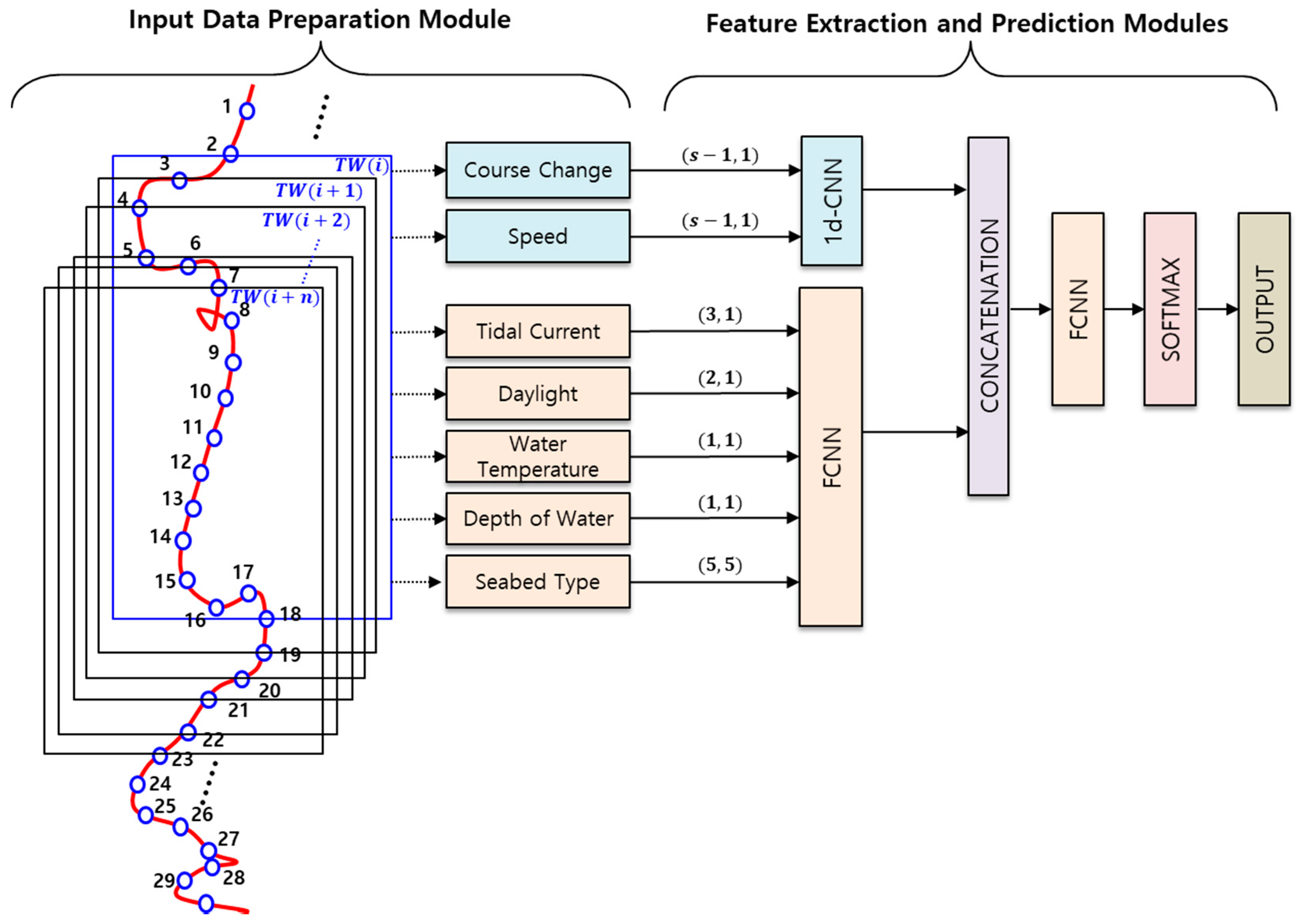
The proposed deep neural network model combines both the 1D CNN model for fishing ship movement and sequential trajectory-pattern learning and the fully connected neural network (FCNN) model for fishing-environment feature extraction, as shown in Figure 4. The proposed model consists of the input data preparation module, the feature extraction module for fishing activity and environments, and the fishing gear type prediction module.

3.4.1. Input Data Preparation Module

AIS data are received in discrete but not regular intervals, and we want to use the processed trajectory data sampled at a regular rate. To handle this problem, we sample the AIS trajectory data. Such sampled trajectory data are pseudo-sample (interpolated) dynamic data which consists of ship position ($pp \left(t_i\right)$), speed ($spd \left(t_i\right)$), and course ($co \left(t_i\right))$ where $t_i$is the $i$-th reference time at which sampling is made according to Section 3.3. A trajectory window $TW\left(i\right)$ consists of a specific number s of consecutive pseudo-sample dynamic data. The reference time points corresponding to trajectory windows are referred to as boundary reference time ($rt$) points. Let $rt\left(i\right)$ denote the boundary reference time point which splits the trajectory segments $TW\left(i-1\right)$ and $TW\left(i\right)$. Suppose that $TW\left(i\right)$ contains consecutive $s$ pseudo-samples. If the boundary reference time point $rt\left(i\right)$ of the trajectory segment $TW\left(i\right)$ is $t_i$, the trajectory segment $TW\left(i\right)$ can be expressed in the sequence of s pseudo-sample dynamic data as follows:

$$TW\left(i\right)=\left(\left[pp\left(t_i\right),co\left(t_i\right),spd\left(t_i\right)\right], \left[pp\left(t_{i+1}\right),co\left(t_{i+1}\right),spd\left(t_{i+1}\right)\right],\dots ,\left[pp\left(t_{i+s}\right),co\left(t_{i+s}\right),spd\left(t_{i+s}\right)\right]\right)$$

(5)

The trajectory windows are constructed by a sliding window scheme in which the following trajectory window starts at the next second segment of the preceding trajectory window. Suppose that the $i$-th trajectory window $TW\left(i\right)$ of size $s$ consists of $TW\left(i\right)=(\left[pp\left(t_i\right),co\left(t_i\right),spd\left(t_i\right)\right],\left[pp\left(t_{i+1}\right),co\left(t_{i+1}\right),spd\left(t_{i+1}\right)\right],\dots ,\left[pp\left(t_{i+s}\right),co\left(t_{i+s}\right),spd\left(t_{i+s}\right)\right]$). Then the next trajectory window $TW\left(i+1\right)$ is set to $W\left(i+1\right)=(\left[pp\left(t_{i+1}\right),co\left(t_{i+1}\right),spd\left(t_{i+1}\right)\right],$ $\left[pp\left(t_{i+2}\right),co\left(t_{i+2}\right),spd\left(t_{i+2}\right)\left],\dots ,\right[pp\left(t_{i+s+1}\right),co\left(t_{i+s+1}\right),spd\left(t_{i+s+1}\right)\right]$). Here, the number of pseudo-samples for a TW window is determined to sufficiently cover the trajectory patterns encompassing their setting, waiting, and hauling phases. In the experiments, a TW window is set to contain 1440 psuedo-samples over about 24 h. Figure 5 represents trajectory window data over the sliding trajectory window.

A ship in fishing activity exhibits a specific trajectory pattern for the fishing gear type while making frequent course direction changes at a low speed. The course change CC ($t_i$) of a ship at a time point $t_i$is defined as the absolute course difference $Cd$($t_i$) between$Co\left(t_{i+1}\right)$ and $Co\left(t_i\right)$ as in Equation (6).

$$\begin{array}{c}Cd(t_i)=\left|Co\left(t_{i+1}\right)-Co\left(t_i\right)\right|\\ CC\left(t_i\right)=\{\begin{array}{cc}360-Cd\left(t_i\right)& \mathrm{if} Cd\left(t_i\right) \ge 180 \\ Cd\left(t_i\right)& \mathrm{otherwise}\end{array}\end{array}$$

(6)

The training data set $FAD\left(i\right)$for the proposed deep-learning model consists of both the sequence of course changes and the sequence of speeds at each sampling time point in the sampling window $TW\left(i\right)$.

$$FAD\left(i\right)=\left(\left[CC\left(t_i\right),CC\left(t_{i+1}\right),\dots ,CC\left(t_{i+s-1}\right)\right], \left[Spd\left(t_i\right),Spd\left(t_{i+1}\right),\dots ,,Spd\left(t_{i+s-1}\right)\right]\right)$$

(7)

There are some environmental factors that affect fishing activities such as daylights, tidal current, water temperature, water depth, and seabed type. The proposed method uses an environmental dataset that contains information of such environmental factors. Some fish are phototactic and hence daylight information is expressed as a binary value where 0 indicates daytime and 1 indicates nighttime. Tidal current speed affects the distributions of planktons of which fish move along, and hence the tidal current speed difference information is used, which is set to the difference between maximum tidal current speed and minimum tidal current speed in the trajectory window. Each fish species has its own favorite water temperature. The environmental data set contains a field for the water temperature, which is a binary value 1 for a temperature of higher than 25° and 0 for other temperatures. Some fish live near the water surface, some live in mid-depth water, and some live near the seabed. The water depth is kept in the environmental data set, where values are set from the range [0, 500] m. The seabed is an important habitat for fish, and some fish like to live in a specific seabed type. The proposed method keeps the information of seabed type for each trajectory window, in which seabed type is one of mud, shell, rock, sand, or gravel.

Table 2. Constitution of training data set.

	Field	Type	Data Size
Ship Movement	Course Change	Continuous	($\mathrm{s}-1$) $\times$ 1
	Speed	Continuous	($\mathrm{s}-1$) $\times$ 1
Fishing Environment	Tidal Current	Continuous	1 $\times$ 1
	Daylight	Categorical (0: Day, 1: Night)	1 $\times$ 1
	Water Temperature	Continuous	1 $\times$ 1
	Water Depth	Continuous	1 $\times$ 1
	Seabed Type	Categorical (0: Mud, 1: Shell, 2: Rock, 3: Sand, 4: Gravel)	5 $\times$ 1

shows the fields of the training data set used in the proposed method. Data consists of fields for ship movement and fishing environment.

3.4.2. Feature Extraction and Prediction Modules

This section describes the feature extraction and prediction modules which extract meaningful features from the preprocessed data and makes predications for fishing gear types. The 1D CNN submodules for the fishing ship movement module extracts $k$features from $\mathrm{s}-1$ preprocessed data records of course change and speed using the deep-learning model of the following architecture:

Input$\left(s-1,1\right)$ − [1D Conv (30) $\times$ ReLU Activation] $\times 2$ − Max Pooling − [1D Conv (30) $\times$ ReLU Activation] $\times 2$ − Max Pooling − Flatten Layer − Output$\left(k,1\right)$

In the architecture, 1D Conv(30) indicates a convolution layer that extracts features from one-dimensional data using 30 convolution filters. 1D Conv is used because input data of course change and speed can be treated as one-dimensional data.

A convolution operation extracts features for an input with the kernel as follows. Suppose that input data ${\mathit{C}}^{n-1}$is one-dimensional data and the kernel ${\mathit{W}}^n$is a one-dimensional array of size, i.e., $K$. Let * denote the convolution operation and $f$ is an activation function with ReLU function [26]. When the convolution kernel ${\mathit{W}}^n$is applied to input ${\mathit{C}}^{n-1}$ then the output ${\mathit{C}}^n$ is computed as follows. Here, ${\mathit{b}}^n$ is a bias term. The parameters of convolution kernels are automatically trained from the training data.

$${\mathit{C}}^n=f\left({\displaystyle \sum }_{i=1}^{{\mathit{C}}_x^{n-1}}{\mathit{C}}_i^{n-1}*{\mathit{W}}_i^n+{\mathit{b}}^n\right)$$

(8)

Max pooling indicates the max pooling operation, and [ ] × 2 indicates the repetition number in the bracket [ ]. It plays the role of selecting maximum feature values and of reducing input into a smaller one. The convolution layers use a $3\times 1$convolution kernel, and max pooling operations are carried out with the $4\times 1$ window. The input is given as $\left(s-1\right)\times 1$ array which represents the fishing ship course change or speed vectors expressed in one channel. Here $s$ is the number of pseudo-samples for the trajectory in a trajectory window data. In the experiments, the length of the trajectory window is 24 h, the sliding trajectory window moves the trajectory down by 3 min, and thus, the number $s$ of pseudo-samples is 480. On the other hand, the output is produced in a $k\times 1$array. Here $k$ is the number of nodes at the output layer of the feature extraction module. In the experiments, $k$ is 3570 (119 × 30).

In the feature extraction module, the other feature extraction component for speed shares the same architecture for the feature extraction component of course change. Figure 6 shows those component outputs which are concatenated into a one-dimensional feature.

The fishing environment data such as tidal current, daylight, water temperature, water depth, seabed type are aggregated into one-dimensional data and then fed into the following FCNN (fully connected neural network) which extracts fishing environment features:

$$Input(9,1)-FCL\left(20\right)-Dropout\left(0.2\right)-FCL\left(20\right)-Dropout\left(0.2\right)-Output\left(20,1\right)$$

here FCL(p) indicates a fully connected layer with $p$ nodes. For each node of a fully connected layer, the input dimension is $m\times 1$ where m is the number of nodes in the preceding layer, and the output dimension is $p\times 1$. In the fully connected layers, each node is connected to all nodes of the preceding layer. The output $N_i^{l+1}$of the $i$-th node at layer l is computed as follows:

$$N_i^{l+1}=f\left({\displaystyle \sum }_{j=1}^n{w}_i^{l+1}{N}_j^l+b_i^{l+1}\right)$$

(9)

here, $w_{\left(i,j\right)}^{l+1}$ is the connection weight between the $i$-th node at layer l and the $j$-th node at layer l +1, $b_i^{l+1}$ is the bias term for the $i$-th node at layer l + 1, and $f$ denotes the activation function. In FCNN, the ReLU activation function is used.

The outputs of the 1D CNN-based feature extraction submodule for ship movement data and the FCNN-based feature extraction module for environmental data are concatenated and passed to the prediction module with the following architecture:

$$Input(60,1)-FCL\left(50\right)-Dropout\left(0.2\right)-FCL\left(30\right)-Dropout\left(0.2\right)-SOFTMAX-Output\left(6,1\right)$$

The prediction module consists of a fully connected network with two hidden layers, each of which has 50 and 30 nodes, respectively, and the output layer has 6 nodes, which equals the number of fishing gear types. The final output is computed by applying the Softmax operation to the computed results of output nodes. Moreover, in order to improve the performance, the proposed modules contain some additional operational layers for batch normalization and dropout operations.

The Softmax operation [27] is computed using Equation (10), which makes the final outputs nonnegative and sum to one.

$$f_k=\frac{\exp ({{\displaystyle \sum }}_{j=1}^m{w}_{jk}{x}_j)}{{{\displaystyle \sum }}_{l=1}^K\exp ({{\displaystyle \sum }}_{j=1}^m{w}_{jl}{x}_j)}$$

(10)

where $f_k$ denotes the final output for the $k$-th node, which corresponds to the probability of the input belonging to the $k$-th fishing gear type. $x_i$ is the output of the i-th node at the preceding layer, $w_{jk}$is the weight between the $j$-th node at the preceding layer and the $k$-th node at the output layer, $m$ is the number of nodes at the preceding layer, and $K$ is the number of nodes (i.e., the number of fishing gear types) at the output layer.

The proposed model is trained to minimize the error function using a gradient descent-based training algorithm. The fishing gear-type classification problem is a kind of multi-class classification problem. The proposed method hence uses the categorical cross-entropy function as the error function $E,$ which is defined as follows [28]:

$$E=-{\displaystyle \sum }_{i=1}^K{t}_i\log f_i$$

(11)

where $t_i$ is the ground truth value for the i-th fishing gear type, and $f_i$ is the final output for the $i$-th fishing gear type, which is computed by the prediction module.

For the performance evaluation of the trained model, the test data was generated from the trajectory data of the days from which the training data was not generated. A total of 480 trajectory window data records $TW\left(i\right)$ of each fishing ship were generated by moving the sliding trajectory window TW by 3 min (length of 24 h per each day) for testing as shown in Figure 4. Among the generated trajectory window records, the records for non-fishing activity are ignored.

We used the performance index TPI, called the trajectory window-wise performance index, which is defined in Equation (12).

$$\mathrm{TPI}=\frac{{{\displaystyle \sum }}_{d=1}^{D_{te}}{{\displaystyle \sum }}_{s=1}^{S_d}{{\displaystyle \sum }}_{n=1}^{K_s^d}\delta \left(f\left(T{W}_s^d\left(n\right)\right), t_s^d\left(n\right)\right)}{{{\displaystyle \sum }}_{d=1}^{D_{te}}{{\displaystyle \sum }}_{s=1}^{S_d}{K}_s^d}$$

(12)

where $D_{te}$ is the number of days for which trajectory data are used for testing, $S_d$ is the number of ships engaged in fishing activity in a specific day $d$, and $K_s^d$ is the number of trajectory window data records for day $d$ and ship $s$. $T{W}_s^d\left(n\right)$ is the n-th trajectory data for day $d$ and ship $s$, $f\left(T{W}_s^d\left(n\right)\right)$ is the fishing gear type for $T{W}_s^d\left(n\right)$, and $t_s^d\left(n\right)$ is the ground-truth fishing gear type for $T{W}_s^d\left(n\right)$. δ (a, b) indicates a function which gives 1 if a = b, otherwise 0. Hence TPI has the range [0, 1]. A higher TPI indicates better accuracy of the trained model.

We also used another performance index DPI, called the day-wise performance index, which is defined in Equation (13).

$$\mathrm{DPI}=\frac{{{\displaystyle \sum }}_{d=1}^{D_{te}}{{\displaystyle \sum }}_{s=1}^{S_d}\delta \left(g\left(T{W}_s^d\right), t_s^d\right)}{{{\displaystyle \sum }}_{d=1}^{D_{te}}{S}_d}$$

(13)

where $g\left(T{W}_s^d\right)$ is the fishing gear type that has the maximum frequency among the fishing gear types, which are suggested by the proposed model for the trajectory window data records of day $d$ and ship $s$. $t_s^d$ is the ground-truth fishing gear type for day $d$ and ship $s$. The fishing gear type of a specific ship is assumed to be fixed on a specific day because it is hard for a ship to carry more than one type of fishing gear at a time. The higher the DPI, the better the accuracy of the trained model.

4. Experiments

4.1. Data Preparation

For the experiments of the proposed method, we used an AIS trajectory data set collected over the one year (year 2016) in a Southern part of the Korean peninsula water area, which covers the Jeju island. The AIS data of size 2.5 giga bytes were collected daily over the water area, and the total size of the data set is approximately 900 giga bytes. The AIS data set contains all types of ships in the water area, of which approximately one-third are fishing ships and the remaining are merchant and other ships. The number of fishing ship records in the AIS data set is 5,865,696,000, including both dynamic and static data for 1380 fishing ships. All the AIS data for each fishing ship are sorted out and trajectories are interpolated according to the method explained in Section 3.3. For training and testing of the classification model, the trajectory data for each ship was created by sampling its interpolated trajectory every 1 min over the trajectory window length of 24 h, where the trajectory window slides over the trajectory by 3 min. The number of trajectory window data was 52,560,000. Eighty percent (292 days) of the data set was used for training, and twenty percent (73 days) of the data set was used for testing. The correlation between the neighboring trajectory windows is very high and hence, in the experiments, the data set was divided into a training data set and a testing data set in a day-wise manner. For example, the trajectory data set of the first 24 days of a month is used for training, and the remaining data set for the following 6 days of the month is used for testing. Among the data sets, the trajectory data records for non-fishing activities like high-speed navigation, and in-harbor area berthing or movements were ignored. Out of the total trajectories, 24,966,000 trajectory windows were used for training and testing.

The AIS data contains information about ship type, in which the fishing ships are labeled with the code ‘30′ that indicates ‘fishing ship’, but the AIS data does not contain information about fishing gear type for the fishing ships. The fishing gear-type information is mandatory for training a fishing gear-type classification model. To get this information, we searched for the fishing gear type of each fishing ship in the Korean Fishing Ship Register Database, which is managed by the National Federation of Fisheries Cooperatives of Korea and to which all fishing ships must register their information, including fishing gear type. In the experiments, we grouped the fishing gear types into 6 classes. Figure 7 shows the experimental procedure for the proposed methods. First, it extracts the AIS data for ships whose ship type is ‘30′ and maintains them for each fishing ship separately. Next, it looks up the Korean Fishing Ship Register Database for the fishing gear type of each ship and augments the fishing gear-type information to the AIS data. After that, it interpolates the trajectories of ships and creates the trajectory data over the sliding window of 24 h. Finally, it partitions the trajectory data set into a training data set and testing data set while ignoring the non-fishing-activity trajectory data.

In the experiments we have used the environmental data set of tidal current, water temperature, water depth, and seabed type, which was collected by the Korea Hydrographic and Oceanographic Agency (KHOA) that conducts ocean observation and hydrographic survey in the Korean waters [29]. KHOA measured those environmental factors in the grid of 5 ${\mathrm{km}}^2$ rectangular regions and stored them in NetCDF (network common data form) format.

4.2. Labeling the Fishing Gear Type

There are 34 fishing gear types in the Korean Fishing Ship Register Database. We ignored 10 fishing gear types for fish-catch transportation ship, fish farm-operating ship, and low-frequency ships in Korean waters, such as long back set net ship, shrimp beam trawl ship, lift net ship, and hanging culture ship. According to their fishing gear similarity, the remaining 21 fishing gear types are grouped into 6 classes: purse seine, stow net, longline, drift gill nets, traps, and single trawl.

Table 3. Fishing gear classification.

Fishing Gear License Type	Fishing Gear Class Groups
The offshore large-scale purse seine	Purse seine
The medium-sized purse seine
The coastal purse seine
The offshore stow net	Stow net
The elver stow net
The improved stow net
The longline	Longline
The offshore longline
The offshore drill gill net	Drift gill net
The offshore drill gill net
The set gill net
The drift gill net
The offshore set gill net
The offshore eel trap	Traps
The offshore trap
The coastal trap
The large-scale trawl	Single trawl
The large-scale bottom trawl
The large steamer’s bottom trawl
The east-sea medium-scale bottom trawl
The large steamer’s pair bottom trawl

shows the groupings of fishing gear license types which are grouped according to their similarities. Each grouped fishing gear type has its own unique characteristics as follows.

For the purse seine gear, the fishing mostly work takes place at night. However, both daytime and night time data for purse seine gear ships have been used for model training and evaluation. The purse seine net is set in a circle and thus the fishing ship makes a cyclic trajectory. It takes less than one hour to set a net and about 3 h to haul the net. The purse seine gear ship catches fish that live near the surface regardless of the depth of the water. The purse seine gear class includes the offshore large-scale purse seine, the medium-sized purse seine, and the coastal purse seine.

For the stow net gear, a stow net tied with anchors is set into the waters where the difference in the tidal range is large, and fish that roam along the tidal current are caught. It takes less than an hour for a stow net gear ship to set the net. The ship waits about 10 h before hauling the net. It takes three to five hours to haul the net. The stow net gear class includes the offshore stow net, the elver stow net, and the improved stow net.

For the longline, the net has many hooks hanging from branching ropes tied to a long rope. The fishing gear is used to catch fish that live at the deep level of the waters. It takes about an hour for a longline ship to set several net lines and five to eight hours to haul them. The longline class includes the longline and the offshore longline.

For the drift gill net gear, drift nets are hung vertically in the water column by floats or a sea anchor attached to a rope. These nets are set when the tidal range difference is mall and where fish pass in the middle and deep depth. It takes two to three hours for a grill net gear ship to set the nets. The ship waits eight to ten hours before hauling the nets. It takes eight to ten hours for the ship to haul the nets. The drift gill net gear class include the offshore drill gill net, the offshore drill gill net, the set gill net, the drift gill net, and the offshore set gill net.

For the trap gear, the nets are funnel-like devices which allow a fish to enter but make it impossible to leave the catching chamber. They are set at regular intervals to catch fish like eels which live on the bottom. It takes one to two hours to set the nets and about 8 h to haul them. The trap gear class includes the offshore eel trap, the offshore trap, and the coastal trap.

For the trawl gear, one or two fishing ships pull a net to catch fish that live in the middle or deep depth of the water. It takes 30 min for setting and hauling the nets and one to three hours to pull the nets. The trawl gear ships moves at the speed of 2 to 4 knots while they are in fishing activities [24]. The trawl gear class includes the large-scale trawl, the large-scale bottom trawl, the large steamer’s dragnet, the large steamer’s pair dragnet, the east-sea medium-scale bottom trawl, and the southwestern-sea bottom pair trawl.

Figure 8 shows the spatial trajectory distributions for each fishing gear types.

4.3. Taining and Performance Evaluation of the Proposed Model

To train the proposed model and evaluate its performance, we used as the training data the 19,972,800 (80%) trajectory window data records for the first 292 days in the available data set and as the test data, the remaining 4,993,200 (20%) trajectory window data records for the following 73 days. For the training data, the portions of each fishing gear type were not uniform as follows: purse seine class 21.2% (4,234,234 records), stow nets class 15.7% (3,135,730 records), longline class 12.4% (2,476,627 records), drift gill nets class 9.2% (1,837,498 records), traps class 18.4% (3,674,995 records), and trawls class 23.1% (4,613,717 records). To resolve the class imbalance problem, we randomly selected 1,000,000 records for each fishing gear type at each training epoch. The portions of each fishing gear type in the test data were also not uniform. Hence, we randomly selected 300,000 records for each fishing gear type from the test data as the validation data set. Once the trained model was obtained, we used the entire test data set to evaluate the trained model.

The performance of the trained models was evaluated with respect to the proposed performance indices TPI and DPI. In the experiment, the proposed model performance was significantly affected by the size of the trajectory window. Figure 9 shows the performance of each type of fishing gear class when the size of the trajectory window is set to 1, 5, 10, 15, 20 and 25 h, respectively.

To evaluate the validity of the proposed method, we also developed an SVM (support vector machine)-based model for the same data set, and compared the performances of the proposed model and the SVM-based model. For the SVM-based model, both course change and speed were discretized into 10 intervals and their histograms were constructed. The histograms and environmental data were used as the input to the SVM-based model. To handle multiple fishing gear classes in the SVM-based model which is a binary classifier, we used the one-versus-rest (OVR) scheme where the classes are fitted against all other classes [30]. There are several kernel functions which can be applied in an SVM model. In the experiments, the following three kernel functions had been examined: sigmoid, polynomial, and linear kernels. For each kernel type, the same experiments had been conducted and the performance of the trained SVM models has been measured. Among the kernel functions, the linear kernel gave the best performance with the hyperparameters of C = 1 and $\mathsf{\gamma }=0.5$.

Table 4. The comparative experiments results of the support vector machine (SVM) model kernel.

	SVM-Based Fishing Gear Type Identification
	Kernel = ‘sigmoid’	Kernel = ‘poly’	Kernel = ‘linear’
Purse Seine	0.917	0.819	0.922
Stow nets	0.670	0.130	0.679
Longline	0.962	0.927	0.953
Drift gill nets	0.728	0.401	0.743
Traps	0.242	0.152	0.399
Trawls	0.922	0.874	0.918
average	0.740	0.525	0.769

shows the performances of the SVM models for different kernel functions. According to the applied kernel function, the SVM models have shown significantly different performances in the experiments.

Table 5. TPI scores for the SVM-based and the convolutional neural network (CNN)-based model.

Label	The Number of Test Data in TW (Percentage)	The SVM-Based Model	The Proposed CNN-Based Model
Purse Seine	1,058,558 (21.2%)	0.922	0.924
Stow Nets	783,932 (15.7%)	0.679	0.845
Longline	619,157 (12.4%)	0.953	0.873
Drift Gill Nets	459,374 (9.2%)	0.743	0.857
Traps	918,749 (18.4%)	0.399	0.931
Trawls	1,153,430 (23.1%)	0.918	0.925
Total	4,993,200	0.769	0.901

shows the TPI scores of the SVM–based model and the CNN-based model for the test data set in which the size of the TW is 24 h. The purse seine, trap, and trawl fishing gear types have TPI scores of more than 0.92 for the CNN-based model. We understand that they seem to have unique characteristic trajectory patterns for setting, hauling and pulling phases. The SVM-based model gave similar performances to the CNN-based model for the purse seine, longline, and trawl types, but the CNN-based model showed superior performance to the SVM-based model for stow net and trap types. The stow net, longline, and gill net fishing gear types have relatively lower TPI scores for the CNN-based model. They seem to have somewhat similar trajectories in their fishing-time spans. The SVM-based model showed worse performance for traps than for purse seine, stow nets, and longline. Fishing ships of trap type have shorter periods for both fishing gear setting and hauling compared to other fishing gear types, and in addition they slow down for fishing gear setting and then move to other trap sites at a speed of more than 6 knots. Hence, the speed histograms of trap type show tall heights both in a high speed range for fishing gear setting and in a low speed range for fishing gear setting and hauling which are also observed in the histograms for stow net, longline, and drift gill net types. The similarities in the histograms of trap type with those of those types and the absence of trajectory information in the speed histograms seem to make it difficult for the SVM model to tell trap type from those types. The SVM-based model classified correctly 39.9% of traps into traps, but incorrectly 2.1% of traps into purse seine, 15.7% into stow nets, 21.4% into longline, 16.4% into drift gill nets, and 2.1% into trawls. The histogram-based features used for the SVM model seems not to be sufficiently good enough to extract meaningful features for traps. On the contrary, the CNN-based model seems to be better at taking into account the continuous changes in speed and course than the SVM-based model. For the longline type, the SVM-based model showed slightly better performance than the CNN-based model. The CNN-based model seems to make some false classification for trajectory windows of longline type due to the temporarily occurring non-fishing periods and the trajectory patterns partially similar to those of stow net and drift gill net types. As shown in

Table 6. Day-wise performance index (DPI) scores for the SVM-based and the CNN-based model.

Label	The Number of Test Data in Days (Percentage)	The SVM-Based Model	The Proposed CNN-Based Model
Purse Seine	7111 (21.4%)	0.935	0.965
Stow Nets	5226 (15.7%)	0.721	0.941
Longline	4195 (12.6%)	0.971	0.955
Drift Gill Nets	3077 (9.3%)	0.782	0.936
Traps	6060 (18.3%)	0.512	0.971
Trawls	7550 (22.7%)	0.968	0.985
Total	33,187	0.814	0.963

, however, the performance of CNN-based model for the longline type comes close to that of the SVM-based model when they were evaluated for TPI scores.

The performance index DPI identifies the fishing gear type for a given trajectory over a day by taking the major gear type for all trajectory window data of which time span are, even partially, overlapped with the time span of the day. Table 6 shows the DPI scores for the trained model. The total performance of DPI is improved by 0.062 compared to that of TPI. The performance for stow net, longline, and drift gill net gear type has been greatly improved by almost 0.5 or more.

Work by Russo et al. [19] used a fishing trip of about two weeks for training and testing and handles three fishing gear types. Their method achieved 94.4% accuracy for the three fishing gear types. Our method achieved 0.963 DPI for a six gear-type classification. Here DPI corresponds to the accuracy for Russo et al.’s method. Our method is superior to their method in that our method uses only fishing trip data over 24 h, handles six fishing gear types, and achieves higher accuracy than their method.

Table 7. Confusion matrix for the experiments of TPI.

		Predicted Label
		Purse Seine	Stow Nets	Longline	Drift Gill Nets	Traps	Trawls
Actual Label	Purse Seine	92.4% (978,213)	1.2% (12,385)	1.9% (20,218)	1.5% (15,349)	1.7% (17,678)	1.4% (14,714)
	Stow Nets	1.2% (9329)	84.5% (662,501)	5.4% (41,940)	6.7% (52,288)	1.3% (9956)	1.0% (7918)
	Longline	0.7% (4582)	5.9% (36,345)	87.4% (541,019)	4.9% (30,772)	0.8% (4829)	0.3% (1610)
	Drift Gill Nets	0.7% (3262)	6.7% (30,824)	5.0% (22,785)	85.7% (393,775)	1.5% (7074)	0.4% (1653)
	Traps	1.3% (11,484)	1.1% (10,106)	2.1% (18,834)	1.2% (10,749)	93.1% (855,723)	1.3% (11,851)
	Trawls	1.7% (19,262)	1.4% (15,687)	1.5% (16,725)	1.5% (17,071)	1.5% (17,417)	92.5% (1,067,268)

shows the confusion matrix for the experiments on TPI. The proposed method has shown good performance with respect to purse seine, trap, and trawl fishing gear type. However, for the stow net, longline, drift gill net fishing gear types, they seem to be confused, and their performance is relatively low.

Figure 10 shows the classification results of the trained model for a trajectory of each fishing gear type. The red tracks indicate the correct classification by the trained model, the sky blue tracks indicate the trajectories of ships with a speed more than 6 knots, which are ignored in the classification, and the tracks in other colors indicate false classification for the corresponding sections.

5. Conclusions

In the marine industry, it is important to estimate the fish catch and to prevent illegal, unreported, and unregulated (IUU) fishing and overfishing. The existing VMS system allows the Vessel Traffic Service officers to monitor the ship movements in real time and to guess their fishing activities only based on their expertise. The proposed fishing gear type identification method allows to identify the fishing activities of ships from their fishing trajectories collected at the VMS system in real time. It makes it possible to compare the identified fishing gear type with the registered fishing gear type which is maintained at the VMS system. The comparison can detect the suspicious ships of IIU fishing. If the times of fishing activities of each ships are maintained at the VMS system, it is also possible to detect the overfishing ships with the help of some estimation method of fishing catch from the fishing activity times.

AIS data of fishing ships provide information of their locations, speeds, and course changes on the fishing journey at a high sampling rate. It is important to identify the fishing gear types of fishing ships from AIS data because they reflect real fishing status for fish catch estimation, IUU fishing, and overfishing.

This paper proposed a deep-learning based method to classify fishing trajectory data into six fishing gear groups. The proposed method has the following characteristics. First, an interpolation method is introduced for trajectory estimation to reduce the noises in AIS data and to recover the missing AIS data. Second, the proposed method makes use of fishing movement and environmental factors such as water temperature, daylight, tidal current, water depth, and seabed type as well as trajectory data. Third, it uses a sliding window technique to capture time series characteristics into the spatial domain and to capture various dynamic movements in trajectories. Fourth, the proposed deep-learning model consists of two feature extraction modules and a prediction module, where a 1D CNN model is used for extracting features from fishing ship movement data, a FCNN is used for extracting features from environmental data, and the FCNN-based prediction module is used to make prediction of fishing gear type from the two feature-extraction modules.

The proposed model was evaluated with respect to the new proposed performance indices TPI and DPI. It showed good performance for purse seine, trap, and trawl fishing gear types, but relatively poor performance for stow net, longline, and drift gill net fishing gear types. In the experiments, we labeled the fishing gear types of fishing ships with the fishing gear type registered to the Korean Fishing Ship Register Database and assumed that fishing ships do not change their fishing gears. The fishing ships using purse seine, trap, and trawl fishing gear types usually do not change their fishing gears. However, fishing ships using stow net, longline, and drift gill net fishing gear types usually have both a primary fishing gear license and a secondary fishing gear license but register only the primary license to the Korean Fishing Ship Register Database. They may change their fishing gears according to fishing ban periods and fish catch, meaning that some trajectory data might be labeled with false fishing gear types for fishing ships with licenses for purse seine, trap, or trawl fishing gear. This may be the cause for the relative poor performance for those fishing gear types. It is expected to have better performances for those fishing gear types once the correct gear types are labeled to the data set.

This paper claims the following contributions. We developed a new classification method for fishing gear type from real-time AIS and environmental data that helps to estimate fish catch from real fishing activities. It also helps to detect IUU fishing and overfishing for preserving marine resources. It allows for monitoring of the fishing activities of unregistered foreign fishing ships and to enforce the regulations applicable to them. When a fishing ship’s fishing gear type is determined, the proposed method only needs to use an AIS trajectory data of 24 h, while the previous VMS data-based method [19] has to use a trajectory data set of more than 15 days.

There remain opportunities for further studies to improve upon the proposed deep-learning model to reduce the sliding window size. In addition, we need to develop the model to deal with more fishing gear types larger than the current 6 fishing gear types. We have used a data set collected over one year, but a larger data set would help to develop a more improved model. We are currently collecting more data sets for further studies.

References

- Fagan, B. Fish on Friday: Feasting, Fasting, and the Discovery of the New World; Basic Books: New York, NY, USA, 2007. [Google Scholar]
- Cochrane, K.; De Young, C.; Soto, D.; Bahri, T. Climate Change Implications for Fisheries and Aquaculture; FAO Fisheries and aquaculture technical paper 530; FAO: Rome, Italy, 2009; 212p. [Google Scholar]
- Polacheck, T. Assessment of IUU fishing for southern bluefin tuna. Mar. Policy 2002, 36, 1150–1165. [Google Scholar] [CrossRef]
- Botsford, L.W.; Castilla, J.C.; Peterson, C.H. The management of fisheries and marine ecosystems. Science 1997, 277, 509–515. [Google Scholar] [CrossRef] [Green Version]
- Pramod, G.; Nakamura, K.; Pitcher, T.J.; Delagran, L. Estimates of illegal and unreported fish in seafood imports to the USA. Mar. Policy 2014, 48, 102–113. [Google Scholar] [CrossRef]
- Marzuki, M.I.; Gaspar, P.; Garello, R.; Kerbaol, V.; Fablet, R. Fishing gear identification from vessel-monitoring-system-based fishing vessel trajectories. IEEE J. Ocean. Eng. 2017, 43, 689–699. [Google Scholar] [CrossRef]
- Um, S.H.; Lee, W.S.; Beak, Y.S.; Lee, K.H. A Study on the Introduction of a New Fishing Vessel Registration System; Korea Maritime Institute: Busan, Korea, 2019; pp. 9–28. [Google Scholar]
- Sundström, A. Covenants with broken swords: Corruption and law enforcement in governance of the commons. Glob. Environ. Change 2015, 31, 253–262. [Google Scholar] [CrossRef] [Green Version]
- Sundström, A. Corruption in the commons: Whfy bribery hampers enforcement of environmental regulations in South African fisheries. Int. J. Commons 2013, 7, 454–472. [Google Scholar] [CrossRef]
- Davie, S.; Lordan, C. Using a Multivariate Approach to Define Irish Métiers in the Irish Sea. Ir. Fish. Investig. 2009, 21, 1–49. [Google Scholar]
- Deng, R.; Dichmont, C.; Milton, D.; Haywood, M.; Vance, D.; Hall, N.; Die, D. Can vessel monitoring system data also be used to study trawling intensity and population depletion? The example of Australia’s northern prawn fishery. Can. J. Fish. Aquat. Sci. 2005, 62, 611–622. [Google Scholar] [CrossRef]
- Mills, C.M.; Townsend, S.E.; Jennings, S.; Eastwood, P.D.; Houghton, C.A. Estimating high resolution trawl fishing effort from satellite-based vessel monitoring system data. ICES J. Mar. Sci. 2007, 64, 248–255. [Google Scholar] [CrossRef] [Green Version]
- Ortiz, M.; Justel-Rubio, A.; Parrilla, A. Preliminary Analyses of the ICCAT VMS Data 2010–2011 to Identifiy Fishing Trip Behavior and Estimate Fishing Effort. Collect. Vol. Sci. Pap. ICCAT 2013, 69, 462–481. [Google Scholar]
- Marzuki, M.I. VMS Data Analyses and Modeling for the Monitoring and Surveillance of Indonesian Fisheries. Ph.D. Thesis, Universite Bretagne Loire, Rennes, France, March 2017. [Google Scholar]
- Piet, G.J.; Quirijns, F.J.; Robinson, L.; Greenstreet, S.P.R. Potential pressure indicators for fishing, and their data requirements. ICES J. Mar. Sci. 2007, 64, 110–121. [Google Scholar] [CrossRef] [Green Version]
- Vermard, Y.; Rivot, E.; Mahevas, S.; Marchal, P.; Gascuel, D. Identifying fishing trip behavior and estimating fishing effort from VMS data using Bayesian Hidden Markov Models. Ecol. Model. 2010, 221, 1757–1769. [Google Scholar] [CrossRef] [Green Version]
- Joo, R.; Bertrand, S.; Tam, J.; Fablet, R. Hidden Markov models: The best models for forager movements? PLoS ONE 2013, 8. [Google Scholar] [CrossRef] [PubMed] [Green Version]
- Bez, N.; Walker, E.; Gaertner, D.; Rivoirard, J.; Gaspar, P. Fishing activity of tuna purse seiners estimated from vessel monitoring system (VMS) data. Can. J. Fish. Aquat. Sci. 2011, 68, 1998–2010. [Google Scholar] [CrossRef]
- Russo, T.; Parisi, A.; Prorgi, M.; Boccoli, F.; Cignini, I.; Tordoni, M.; Cataudella, S. When behaviour reveals activity: Assigning fishing effort to métiers based on VMS data using artificial neural networks. Fish. Res. 2011, 111, 53–64. [Google Scholar] [CrossRef]
- Tassetti, A.N.; Ferrà, C.; Fabi, G. Rating the effectiveness of fishery-regulated areas with AIS data. Ocean Coast. Manag. 2019, 175, 90–97. [Google Scholar] [CrossRef]
- International Maritime Organization (IMO). Guidelines for the Onboard Operational Use of Shipborne Automatic Identification Systems (AIS); Res A.917; International Maritime Organization (IMO): London, UK, 2002. [Google Scholar]
- Kim, K.I.; Lee, K.M. Deep learning-based caution area traffic prediction with automatic identification system sensor data. Sensors 2018, 18, 3172. [Google Scholar] [CrossRef] [Green Version]
- Sang, L.Z.; Yan, X.P.; Wall, A.; Wang, J.; Mao, Z. CPA calculation method based on AIS position prediction. J. Navig. 2016, 69, 1409–1426. [Google Scholar] [CrossRef]
- Ferrà, C.; Tassetti, A.N.; Grati, F.; Pellini, G.; Polidori, P.; Scarcella, G.; Fabi, G. Mapping change in bottom trawling activity in the Mediterranean Sea through AIS data. Mar. Policy 2018, 94, 275–281. [Google Scholar] [CrossRef]
- Kim, D.S.; Arsalan, M.; Park, K.R. Convolutional Neural Network-Based Shadow Detection in Images Using Visible Light Camera Sensor. Sensors 2018, 18, 960. [Google Scholar] [CrossRef] [Green Version]
- Nair, V.; Hinton, G.E. Rectified linear units improve restricted boltzmann machines. In Proceedings of the 27th International Conference on Machine Learning (ICML-10), Haifa, Israel, 21–24 June 2010; pp. 807–814. [Google Scholar]
- Gao, B.; Pavel, L. On the Properties of the Softmax Function with Application in Game Theory and Reinforcement Learning. arXiv 2017, arXiv:1704.00805. [Google Scholar]
- Robert, C. Machine Learning, a Probabilistic Perspective; The MIT Press: Cambridge, MA, USA, 2014; pp. 62–63. [Google Scholar]
- Korea Hydrographic and Oceanographic Agency. Available online: http://www.khoa.go.kr (accessed on 24 February 2020).
- Xu, J. An extended one-versus-rest support vector machine for multi-label classification. Neurocomputing 2011, 74, 3114–3124. [Google Scholar] [CrossRef]
Figure 1.
Trajectories of fishing and non-fishing activities. (a) Steaming (non-fishing), (b) waiting (non-fishing), (c) setting (fishing), and (d) hauling (fishing): the black tracks indicate a section with a speed of 6 knots or more and red tracks indicate ones with a speed of less than 6 knots.
Figure 2.
Real positions and sampled positions on the interpolated path.
Figure 3.
Ship speed distributions for fishing gear types over the time spans: the morning time span of 5:00 to 12:00 in blue, the afternoon time span of 12:00 to 20:00 in black, and the night time span of 20:00 to 5:00 in red.