Numerical Study of a Customized Transtibial Prosthesis Based on an Analytical Design under a Flex-Foot® Variflex® Architecture

 , ,
, , 
 and
and
Abstract
:Featured Application
Abstract
1. Introduction
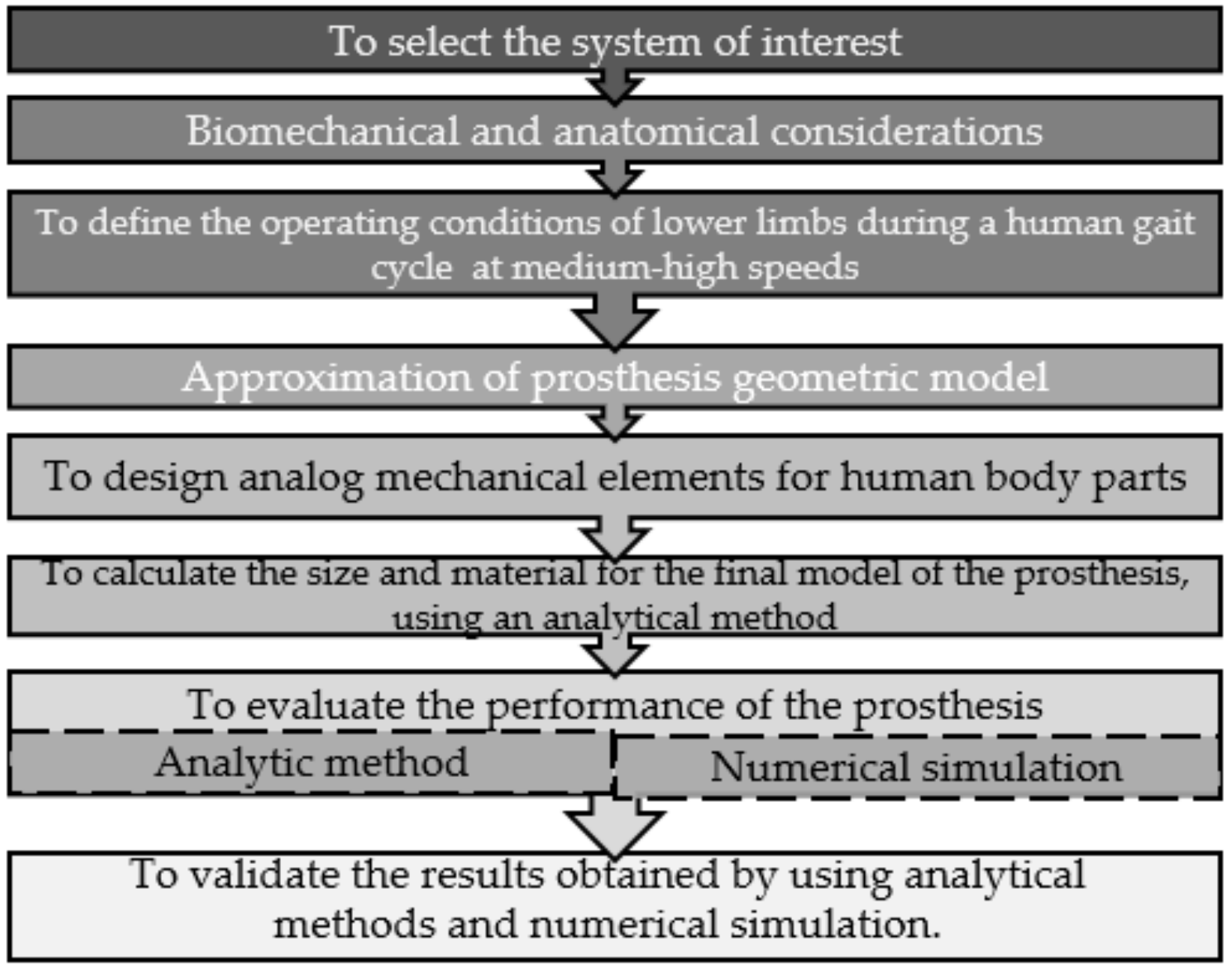
2. Materials and Methods
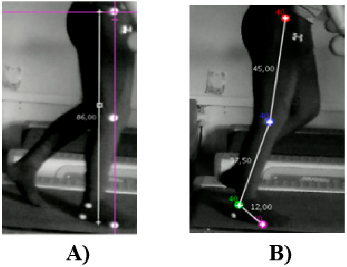
2.1. Biomechanical and Anatomical Considerations
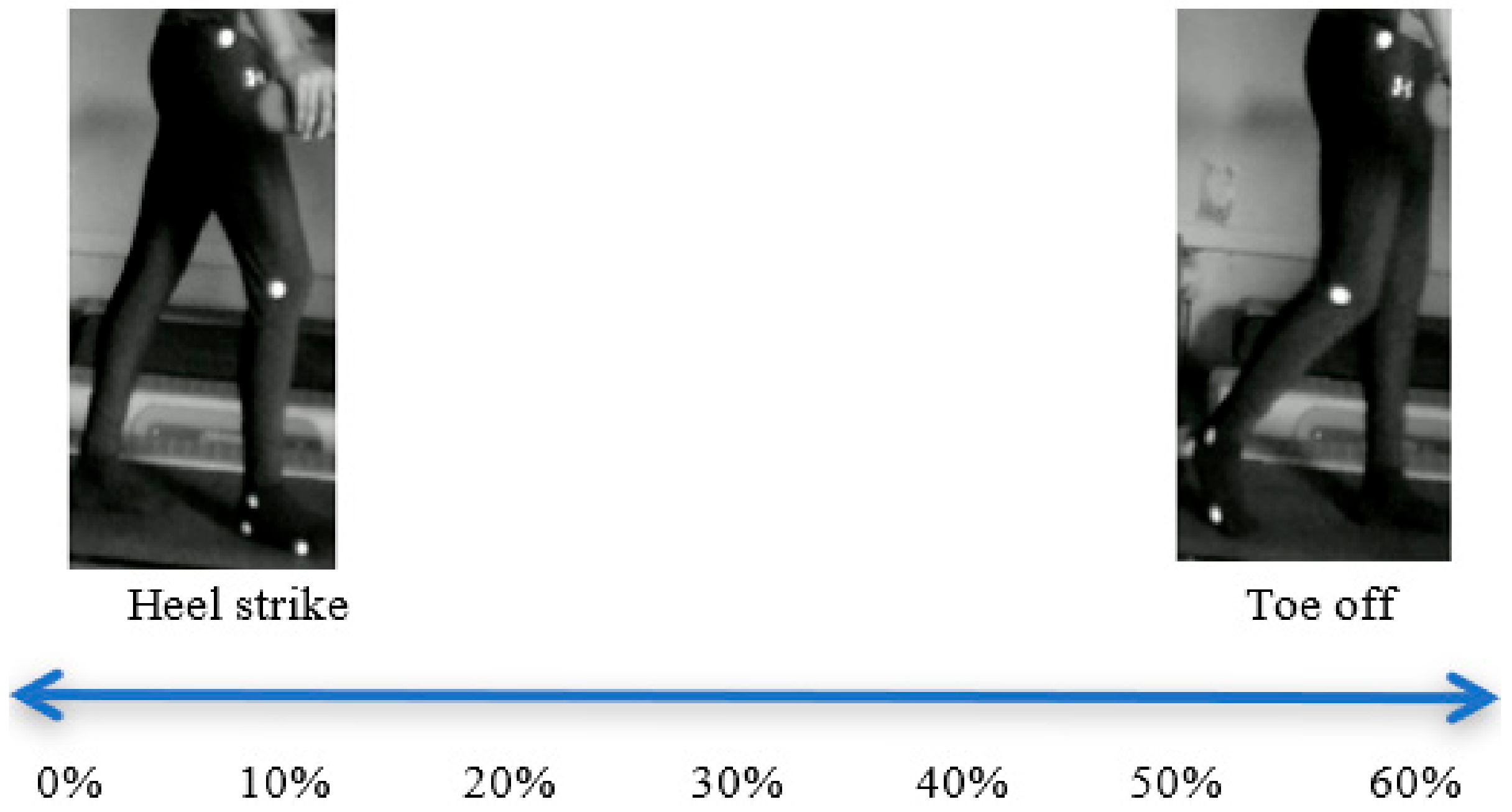
2.2. Conditions of the Lower Limbs during the Gait Cycle
2.2.1. Kinematics
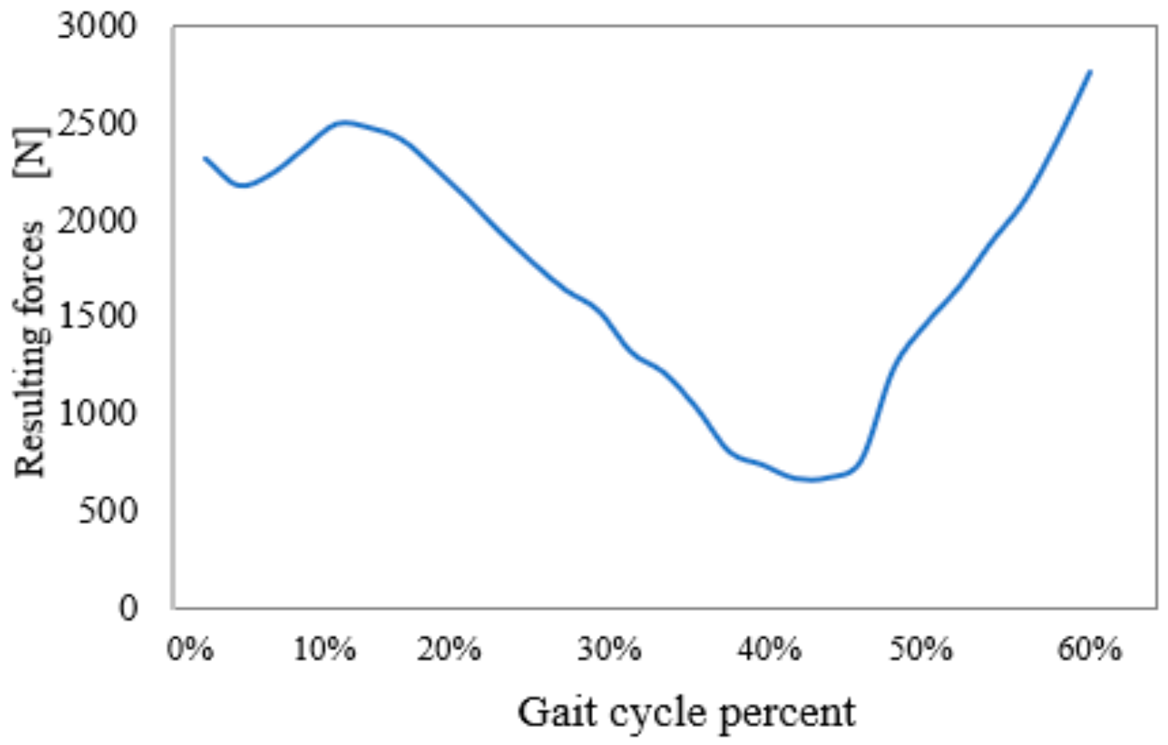
2.2.2. Kinetics
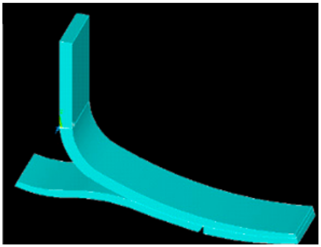
2.3. Approximation of the Geometric Model of the Prosthesis
2.4. Analogy between the Human Body Parts and Mechanical Elements
Material Selection
2.5. Analytical Behavior of the Prosthesis
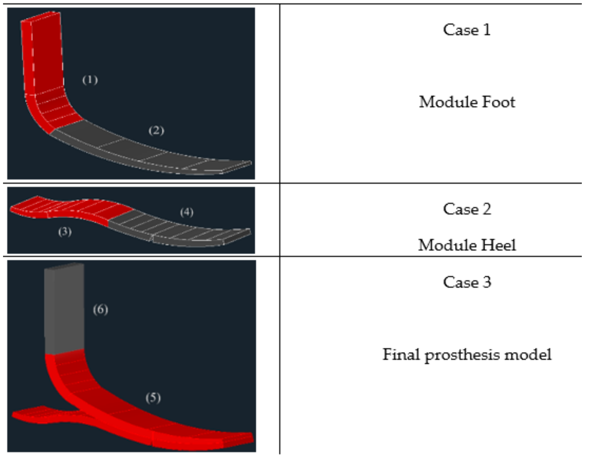
2.5.1. Case 1: Summation of Forces on the Foot Module

2.5.2. Case 4: Articulated Section

2.6. Numerical Prosthesis Assessment
Case 3: Final Prosthesis Model
- Case 3.1: Analysis in the gait subphase when the heel contacts the ground.
- Case 3.2: Analysis in the gait subphase when the heel does not contact the ground.
3. Results
3.1. Lower Limb Operating Conditions during a Gait Cycle at a Medium Speed
3.2. Analytical Assessment of Prosthesis Behavior
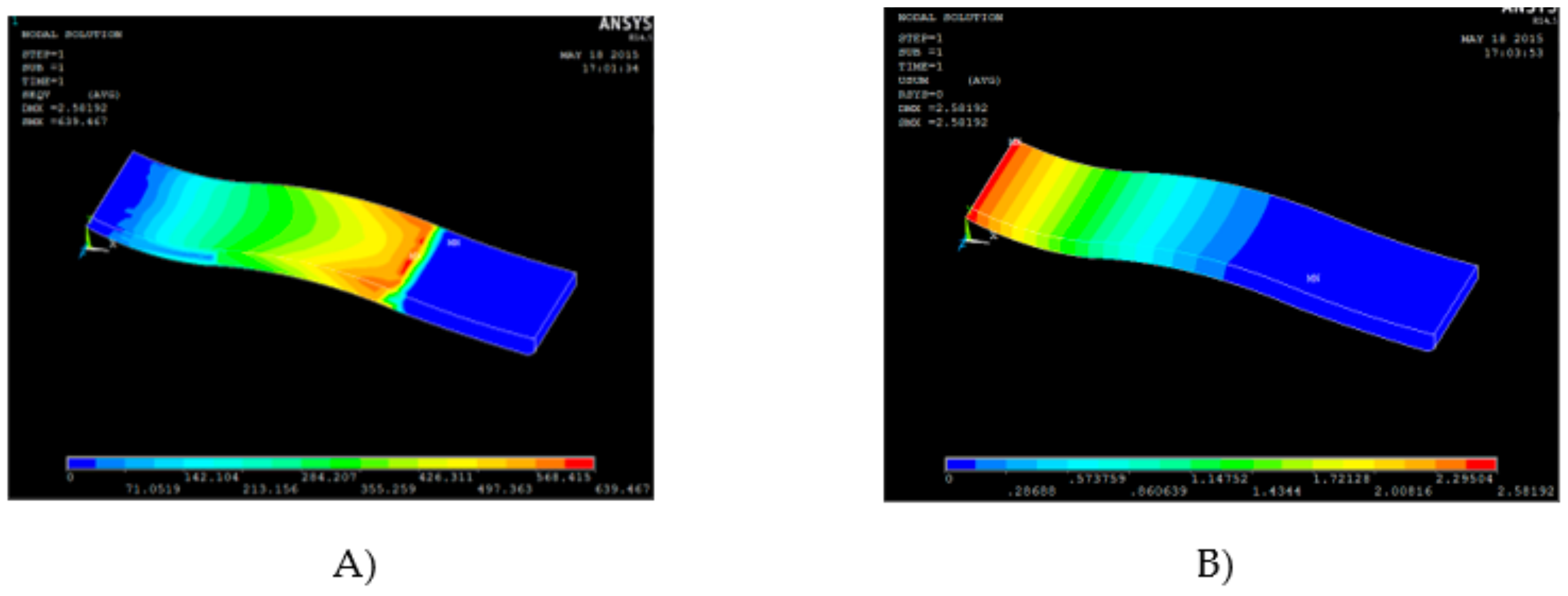
3.3. Numerical Assessment of Prosthesis Behavior
4. Discussion
5. Conclusions
Author Contributions
Funding
Acknowledgments
Conflicts of Interest
References
- International Diabetes Federation. Atlas de Diabetes, 5th ed.; International Diabetes Federation: Brussels, Belgium, 2012; Available online: https://www.idf.org/e-library/epidemiology-research/diabetes-atlas/20-atlas-5th-edition.html (accessed on 1 May 2020).
- Hernández-Ávila, M.; Gutiérrez, J.P.; Reynoso-Noverón, N. Diabetes Mellitus en México. El Estado de la Epidemia. Salud Publica de México 2013, 5, 129–136. Available online: http://www.scielo.org.mx/scielo.php?script=sci_arttext&pid=S0036-36342013000800009 (accessed on 1 May 2020). [CrossRef] [Green Version]
- Su, P.-F.; Gard, S.A.; Lipschutz, R.D.; Kuiken, T.A. Gait characteristics of persons with bilateral transtibial amputations. J. Rehabil. Res. Dev. 2007, 44, 491–502. [Google Scholar] [CrossRef] [PubMed]
- Wang, J.; Zielińska, T. Gait features analysis using artificial neural networks testing the footwear effect. Acta Bioeng. Biomech. 2017, 19. [Google Scholar] [CrossRef]
- Bober, T.; Dziuba, A.; Kobel-Buys, K.; Kulig, K. Gait characteristics following Achilles tendon elongation: The foot rocker perspective. Acta Bioeng. Biomech. 2008, 10, 37. Available online: http://www.actabio.pwr.wroc.pl/Vol10No1/Art_05.pdf (accessed on 1 May 2020).
- Fridman, A.; Ona, I.; Isakov, E. The influence of prosthetic foot alignment on transtibial amputee gait. Prosthet. Orthot. Int. 2003, 27, 17–22. [Google Scholar] [CrossRef] [PubMed] [Green Version]
- Lemaire, E.D.; Samadi, R.; Goudreau, L.; Kofman, J. Mechanical and biomechanical analysis of a linear piston design for angular-velocity-based orthotic control. J. Rehabil. Res. Dev. 2013, 50, 43–52. [Google Scholar] [CrossRef] [PubMed]
- Umberger, B.R.; Martin, P.E. Mechanical power and efficiency of level walking with different stride rates. J. Exp. Biol. 2007, 210, 3255–3265. [Google Scholar] [CrossRef] [PubMed] [Green Version]
- Dorn, T.W.; Schache, A.G.; Pandy, M.G. Muscular strategy shift in the human running: Dependence of running speed on hip and ankle muscle performance. J. Exp. Biol. 2012, 215, 1944–1956. [Google Scholar] [CrossRef] [PubMed] [Green Version]
- Noce-Kirkwood, R.; de Alencar-Gomes, H.; Ferreira-Sampaio, R.; Culham, E.; Costigan, P. Biomechanical analysis of hip and knee joints during gait in elderly subjects. Acta Ortop. Bras. 2007, 15, 267–271. [Google Scholar] [CrossRef] [Green Version]
- Wolf, E.J.; Everding, V.Q.; Linberg, A.L.; Schnall, B.L.; Czerniecki, J.M.; Gambel, J.M. Assessment of transfemoral amputees using C-Leg and Power Knee for ascending and descending inclines and steps. J. Rehabil. Res. Dev. 2012, 49, 831–842. [Google Scholar] [CrossRef] [PubMed]
- McGibbon, C.A. A biomechanical model for encoding joint dynamics: Applications to transfemoral prosthesis control. J. Appl. Physiol. 2012, 112, 1600–1611. [Google Scholar] [CrossRef] [PubMed] [Green Version]
- Zhang, M.; Mak, A.F.T.; Roberts, V.C. Finite element modelling of a residual lower limb in a prosthetic socket: A survey of the development in the first decade. Med. Eng. Phys. 1998, 20, 360–373. [Google Scholar] [CrossRef]
- Silverthorn, M.B.; Childress, D.S. Parametric analysis using the finite element method to investigate prosthetic interface stresses for persons with trans-tibial amputation. J. Rehabil. Res. Dev. 1996, 33, 227–238. Available online: https://0-www-ncbi-nlm-nih-gov.brum.beds.ac.uk/pubmed/8823671 (accessed on 1 May 2020).
- Zhang, M.; Lord, M.; Turner-Smith, A.R.; Roberts, V.C. Development of a nonlinear finite element modeling of the below-knee prosthetic socket interface. Med. Eng. Phys. 1995, 17, 559–566. [Google Scholar] [CrossRef]
- Zachariah, S.G.; Sanders, J.E. Finite element estimates of interface stress in the transtibial prosthesis using gap elements are different from those using automated contact. J. Biomech. 2000, 33, 895–899. [Google Scholar] [CrossRef]
- Lee, W.C.C.; Zhang, M.; Jia, X.; Cheung, J.T. Finite element modeling of the contact interface between transtibial residual limb and prosthetic socket. Med. Eng. Phys. 2004, 26, 655–662. [Google Scholar] [CrossRef] [PubMed] [Green Version]
- Jia, X.; Zhang, M.; Lee, W.C.C. Load transfer mechanics between transtibial prosthetic socket and residual limb—Dynamic effects. J. Biomech. 2004, 37, 1371–1377. [Google Scholar] [CrossRef] [PubMed] [Green Version]
- Saunders, M.M.; Schwentker, E.P.; Kay, D.B.; Bennett, G.; Jacobs, C.R.; Verstraete, M.C.; Njus, G.O. Finite element analysis as a tool for parametric prosthetic foot design and evaluation. Technique development in the solid ankle cushioned heel (SACH) foot. Comput. Method Biomech. Biomed. Eng. 2003, 6, 75–87. [Google Scholar] [CrossRef] [PubMed]
- Mara, G.E.; Harland, A.R.; Mitchell, S.R. Virtual modelling of a prosthetic foot to improve footwear testing. Institution of Mechanical Engineers. Part L J. Mater. Des. Appl. 2006, 22, 207–213. [Google Scholar] [CrossRef] [Green Version]
- Özkaya, N.; Nordin, M.; Goldsheyder, D.; Leger, D. Fundamentals of Biomechanics: Equilibrium, Motion, and Deformation, 3rd ed.; Springer-Verlag: New York, NY, USA, 2012. [Google Scholar] [CrossRef] [Green Version]
- Voegeli, A.V. Lecciones Básicas de Biomecánica del Aparato Locomotor, 1st ed.; Springer-Verlag Iberica: Barcelona Spain, 2004; pp. 35–47, 67–74. [Google Scholar]
- Boresi, P.A.; Schmidt, R.J. Advanced Mechanics of Materials, 6th ed.; John Wiley & Sons, New york, USA 2003. Available online: https://www.brijrbedu.org/Brij%20Data/Advance%20Mechanics%20of%20Solids/Book/Advanced%20Mechanics%20of%20Solids%20By%20Arthur%20P%20Boresi%20&%20Schmidth%206%20Ed.pdf (accessed on 1 May 2020).


| Patient | Subject of Study | ||
|---|---|---|---|
| Age | 23 years | Age | 24 years |
| Weight | 70.5 kg | Weight | 73 kg |
| Total height | 173 m | Total height | 174 m |
| Hip to knee length | 44.8 cm | Hip to knee length | 45 cm |
| Knee to ankle length | 37.4 cm | Knee to ankle length | 37.5 cm |
| Ankle to heel length | 8.5 cm | Ankle to heel length | 8.5 cm |
| Hip to heel length | 90.7 cm | Hip to heel length | 91 cm |
| Type of amputation | Transtibial Burgess |
| Study Cases | Maximum Stress Angle (Degrees) | Maximum Stress in Tension (N/m2) | Maximum Stress in Compression (N/m2) |
|---|---|---|---|
| Case 1: Foot Module | 54° | 357,984,296 | −319,161,066 |
| Case 2: Heel Module | 27° | 675,166,712 | −664,295,733 |
| Case 3: Heel Module | 31° | 936,355,844 | −8989,98,77 |
| Prosthesis Section | Max. Deformation (Meters) | |
|---|---|---|
| Cross Section Minimum | Cross Section Maximum | |
| Case 1: Foot Module | 1.02 × 10⁻³ | 0.794 × 10⁻³ |
| Case 2: Heel Module | 2.07 × 10⁻³ | 0.776 × 10⁻³ |
| Case 3: Heel Module | 2.64 × 10⁻³ | 1.79 × 10⁻³ |
| Prosthesis Section | Stress in MPa | ||
|---|---|---|---|
| Analytical Method | Numerical Simulation | Error Rate | |
| Foot module | 357.984296 | 382.812 | 6.4856% |
| Heel module | 675.166712 | 639.467 | 5.2875% |
| Prosthesis Section | Deformations in m | ||
|---|---|---|---|
| Analytical Method | Numerical Simulation | Error Rate | |
| Foot module | 1.02 × 10⁻³ | 9.9866 × 10⁻⁴ | 2.0914% |
| Heel module | 2.64 × 10⁻³ | 2.5819 × 10⁻³ | 2.2% |
© 2020 by the authors. Licensee MDPI, Basel, Switzerland. This article is an open access article distributed under the terms and conditions of the Creative Commons Attribution (CC BY) license (http://creativecommons.org/licenses/by/4.0/).
Share and Cite
Hernández-Acosta, M.A.; Torres-San Miguel, C.R.; Piña-Díaz, A.J.; Paredes-Rojas, J.C.; Aguilar-Peréz, L.A.; Urriolagoitia-Sosa, G. Numerical Study of a Customized Transtibial Prosthesis Based on an Analytical Design under a Flex-Foot® Variflex® Architecture. Appl. Sci. 2020, 10, 4275. https://0-doi-org.brum.beds.ac.uk/10.3390/app10124275
Hernández-Acosta MA, Torres-San Miguel CR, Piña-Díaz AJ, Paredes-Rojas JC, Aguilar-Peréz LA, Urriolagoitia-Sosa G. Numerical Study of a Customized Transtibial Prosthesis Based on an Analytical Design under a Flex-Foot® Variflex® Architecture. Applied Sciences. 2020; 10(12):4275. https://0-doi-org.brum.beds.ac.uk/10.3390/app10124275
Chicago/Turabian StyleHernández-Acosta, Marco Antonio, Christopher René Torres-San Miguel, Armando Josue Piña-Díaz, Juan Carlos Paredes-Rojas, Luis Antonio Aguilar-Peréz, and Guillermo Urriolagoitia-Sosa. 2020. "Numerical Study of a Customized Transtibial Prosthesis Based on an Analytical Design under a Flex-Foot® Variflex® Architecture" Applied Sciences 10, no. 12: 4275. https://0-doi-org.brum.beds.ac.uk/10.3390/app10124275