Assessing the Performance of the Multi-Beam Echo-Sounder Bathymetric Uncertainty Prediction Model


Acoustics Group, Faculty of Aerospace Engineering, Delft University of Technology, 2629 HS Delft, The Netherlands
*
Author to whom correspondence should be addressed.
Appl. Sci. 2020, 10(13), 4671; https://0-doi-org.brum.beds.ac.uk/10.3390/app10134671
Submission received: 10 June 2020
/
Revised: 1 July 2020
/
Accepted: 3 July 2020
/
Published: 7 July 2020
(This article belongs to the Special Issue Modelling, Simulation and Data Analysis in Acoustical Problems Ⅱ)
Abstract
:Realistic predictions of the contribution of the various sources affecting the quality of the bathymetric measurements prior to a survey are of importance to ensure sufficient accuracy of the soundings. To this end, models predicting these contributions have been developed. The objective of the present paper is to assess the performance of the bathymetric uncertainty prediction model for modern Multi-Beam Echo-Sounder (MBES) systems. Two datasets were acquired at water depths of 10 and 30 with three pulse lengths equaling 27, 54, and 134 in the Oosterschelde estuary (The Netherlands). The comparison between the bathymetric uncertainties derived from the measurements and those predicted using the current model indicated a relatively good agreement except for the most outer beams. The performance of the uncertainty prediction model improved by accounting for the most recent insights into the contributors to the MBES depth uncertainties, i.e., the Doppler effect, baseline decorrelation (accounting for the pulse shape), and the signal-to-noise ratio.
1. Introduction
Reliable representation of the sea- and river-floor bathymetry is of high importance for a large number of applications, such as maintaining safe navigation, marine geology, off-shore construction, and habitat mapping [1,2,3]. Acoustic remote sensing with Multi-Beam Echo-Sounder (MBES) systems has been extensively used for delivering such information due to the systems’ capability to map large areas in a relatively short period of time. The system transmits an acoustic pulse (ping) in a wide swath perpendicular to the sailing direction [4]. Beamforming at reception enables determining the Two-Way Travel Time (TWTT) of the received signal for a set of predefined beam angles. The depth measurements are derived from the TWTT per beam and speed of sound in the water [5]. However, similar to any type of measured parameter, the derived depths are affected by varying sources of uncertainty, such as those in the sound speed, motion, and rotation sensors.
Obtaining a realistic a priori estimate of the depth uncertainties is of importance for a number of applications. Approaches to obtain these estimates, and subsequently to use them, are described in the literature. Hare [6,7] developed an a priori vertical uncertainty prediction model to quantify the contribution of various sources. The developed model has been widely used for predicting the uncertainties prior to a survey, as implemented in the A priori Multi-beam Uncertainty Simulation Tool (AMUST) used throughout this paper. Therefore, in this paper, the term uncertainty prediction model refers to the model of [6,7]. This model has been also employed for producing bathymetry maps (for example in the Combined Uncertainty and Bathymetry Estimator (CUBE) algorithm) [8,9,10] and for bridge risk management and coastal inundation modeling [11,12]. Moreover, a realistic bathymetric uncertainty description is key for survey planning to assess whether the required survey standards can be met in a specific measurement campaign.
Apart from the direct application of the depth measurements for map production, derivatives of the bathymetric measurements, such as the slope and bathymetry position index, can be used for sediment classification [13,14]. As an example, Eleftherakis et al. [15,16] combined the so-called depth residuals (related to the depths’ standard deviation) with backscatter strength measurements to increase the discrimination performance of the sediment classification methods and to solve the ambiguity in the relationship between backscatter value and median grain size [17]. Recently, Gaida et al. [18] used the bathymetry uncertainty to assess the statistical significance of the changes in the measured depth differences between the various frequencies with the incident angle. Lacking information with regard to the uncertainties inherent to the MBES can lead to misinterpretation. As an example, on might mistakenly classify the uncertainties and assign different sediment types to measurements having actually the same sediment composition, but different uncertainties.
Effort has been put forward to address the contribution of the uncertainty sources, of relevance to the MBES bathymetric measurements, not accounted for in the uncertainty prediction model of [6,7]. These contributions can result from developments that have been since then realized in MBES systems, such as enabling the use of Frequency Modulated (FM) pulse shapes or using sophisticated bottom detection methods or filters [19,20]. Mohammadloo et al. [21,22] quantified the vertical uncertainties induced by the use of FM pulse shapes and assessed their relevance for MBES bathymetric uncertainty predictions. Lurton and Augustin [4] proposed a unified definition of a quality factor for sonar bathymetry measurements, which is a posteriori estimator of the relative depth uncertainty induced by the signal features. Maleika [23] investigated the impact of varying parameters, such as the vessel speed, swath width, track configuration, and density of the measurements on the final bathymetric grid using a virtual survey simulator.
Despite an impressive amount of research carried out toward theoretical and empirical modeling of the MBES bathymetric uncertainties, there has been little effort to validate the often used bathymetry uncertainty prediction model in varying conditions (either environmental or MBES settings). Comparison between the measured and modeled uncertainties provides one with insight into how realistic the modeling is and can also give directions for future improvements of the bathymetric uncertainty prediction model. This can be also beneficial for the approaches relying on the modeled uncertainty to give an estimate of the soundings’ uncertainty in a grid, such as the CUBE [9,10,24]. These issues have motivated us to assess the performance of the bathymetric uncertainty prediction model by comparing the modeled and measured vertical uncertainties for current state-of-the-art MBES systems and seek for improvements.
This paper is organized as the following. In Section 2, a method for obtaining the depth uncertainties from the measurements such that a fair comparison with the modeled uncertainties can be made is presented. The description of the datasets is given in Section 3. We present the results in Section 4 and discuss the relevant issues. Concluding remarks of this paper are given in Section 5.
2. Modeling and Measuring Bathymetric Uncertainties
2.1. Modeling Approach
The predictions of the depth uncertainty induced by varying sources were derived from the model presented in [6,7]. This model was developed under the assumption of independent contributors (total uncertainty is the square root of sum of the squares of the individual uncertainty sources) and a flat bottom. The bathymetric uncertainty sources can be categorized as [25]:
- Echosounder contribution, , due to the non-zero beam opening angle in the along-track direction, uncertainties in the measurements of the range (between the transducer and a point on the seafloor), and the angle of impact of the incoming sound at the transducer. The latter depends on the method used within the MBES processing chain for bottom detection, i.e., using the amplitude and phase of the received signal. The former is obtained either from the maximum amplitude of the received signal or the center of gravity of the signal envelope after beamforming [26]. As for the phase detection, the full MBES receiving array is divided into two sub-arrays [4]. First, the received signals on both sub-arrays are beamformed focusing the two sub-arrays in a desired direction. The time at which the two signals are in phase (zero phase difference between the two beams formed in a chosen direction) is then taken as the arrival time [4].
- Angular motion sensor contribution, , due to the uncertainties in roll and pitch measurements and the imperfectness of their corrections.
- Motion sensor and echosounder alignment contribution, , due to the discrepancies between roll and pitch angle measurements at the motion sensor and the transducer.
- Sound speed contribution, , due to the sound speed uncertainties at the transducer array and in the water column.
- Heave contribution, , due to the uncertainties in the heave measurements and those induced due to the vertical motion of the transducer with respect to the vertical reference unit caused by the angular motions of the vessel.
For uncorrelated contributors, the total depth uncertainty is then expressed as:
2.2. Determining the Bathymetric Uncertainties from the Measurements
The uncertainty prediction model is based on the assumption of a flat seafloor. Therefore, when comparing the modeled uncertainties with those measurements, areas have to be selected with minimum variation in the water depth. Still, small changes in water depth might be present. To mitigate the contribution of these small variations to the measured uncertainties such that they are comparable to the modeled uncertainties, the approach described in the following is taken.
Measurements in a discrete surface patch on the bottom (with the number of soundings in a surface patch) are considered. The surface patch includes a few angles around the central beam angle and a few consecutive pings. , , and indicate the across-track and along-tack coordinates in the vessel frame along with the depth of the sounding located in the surface patch, respectively. The surface patch is modeled assuming either a plane (with three unknowns) or bi-quadratic polynomial (with six unknowns). Thus, we have [27]:
where the term in the parentheses is used when considering a bi-quadratic polynomial and discarded otherwise. The unknown parameters can be derived from the least-squares method [28]. The least-squares estimate of the unknown parameters for a linear model of observation equations, , with the expectation operator, the design matrix, and the vector containing the observations , is:
where A is of the size with its row being . is the covariance matrix of , with the variance of the data and an identity matrix. For this special structure of covariance matrix (independent and identically distributed errors), Equation (3) is simplified to . The least-squares estimate of the variance component is:
with the -vector of the least-squares residuals [28]. The square root of the variance component gives the estimate of the standard deviation of the depth measurements for which the potential remaining presence of the slopes has been accounted.
3. Description of the Dataset
For validating the depth uncertainty model, a dedicated survey was carried out by the Ministry of Infrastructure and Water Management of The Netherlands (Rijkswaterstaat) in the Oosterschelde estuary (Eastern Scheldt), The Netherlands. This estuary is located in the province of Zeeland, between Schouwen-Duiveland and Tholen on the north and Noord-Beveland and Zuid-Beveland on the south. The survey areas were selected so as to differ in water depth, while the water depth was close to constant within each area. This allowed for experimentally investigating the effect of water depth on the uncertainties and comparing the measured trends with those predicted. The second parameter that was changed during the survey was the pulse length, as this parameter is known to have an important influence on the uncertainties. The EM2040C dual head [29] from Kongsberg was used with the dual swath acquisition and the equiangular beam spacing modes enabled [30], see Table 1.
A brief discussion on the systems used for data acquisition and bathymetry processing is in order. A critical element for accurate estimation of the depth below the transducer is the Sound Speed Profile (SSP) in the water column, which varies both spatially and temporally. Therefore, sufficient and accurate measurements of SSPs are required. To ensure the former, the surveyor was asked to acquire a new SSP in case of a difference of more than 2 / between the surface sound speed value and the sound speed from the latest full SSP [31]. The sound velocity profiler was manufactured by AML oceanographic, and the uncertainty of its measurements as indicated by the manufacturer was /, [32]. However, from measurements in different locations (inland waterways and the North Sea), the uncertainty was found to be /, and hence, this value was chosen as a more realistic description of the system’s uncertainty. The sound speed profiles acquired for both datasets were almost constant in the water column equaling 1515 / and used in the uncertainty prediction model for the sound speed in the water column and at the receiving array.
The datasets were acquired using the Quality Integrated Navigation System (QINSy) (developed by Quality Positioning Services, QPS, BV), and Global Navigation Satellite System (GNSS) sensors received the correction signal from Real-time Kinematic (RTK) services, Netherlands Positioning Service (NETPOS). Using RTK for the vertical positioning in QINSy meant that the depth relative to the chart/vertical datum was directly measured from accurate GNSS observations (For more information on different depth processing algorithms available in QINSy, the interested reader may refer to [33]). Therefore, the water surface level was of no relevance, and accounting for height offsets, such as tide, draft, and height above draft reference, was not necessary as they did not affect the quality of the derived depths. Heave measurements (short-term variations in the transducer depth) were, however, used within the processing software to calculate the height of the vessel center of gravity between two position updates (as the update rate of the Inertial Navigation Sensor (INS) is higher than that of the GNSS system). Therefore, the accuracy of heave measurements acquired by the INS contributed to the uncertainty in the depth estimate. Phins manufactured by iXblue [34] was used as the INS for providing position, true heading, attitude, speed, and heave. The roll and pitch uncertainties of the system were (similarly, the misalignment uncertainties were assumed to be ).
Generally speaking, degradation in the quality of the MBES bathymetric measurements is not solely due to the uncertainties inherent to the MBES. Systematic error sources, categorized as static and dynamic, also contribute (see [35] for a detailed discussion and [24] for a brief explanation). These errors lead to depth errors through the systematic rise and fall of all the beams, see [35,36]. Correcting the measurements for the systematic errors is often carried out using patch tests, correlation analysis between the motion time series, and depth derivatives or assessing the agreement between the depth measurements at the overlapping parts of the adjacent swaths [36,37,38]. By using these investigation tools, we concluded that the variations of the depth measurements in the surveyed areas were not caused by the systematic error sources.
For the data acquisition, a Continuous Wave (CW) pulse type was used with a total pulse length, T, equaling 27 , 54 , and 134 (corresponding to the effective pulse length of [39]). Measurements were taken at depths of around 10 and 30 , along tracks of nearly 760 and 640 in length, respectively. Shown in Figure 1 are the bathymetry maps, derived from Qimera (developed by QPS BV), for the water depths of 10 (c) and 30 (d). These were based on the measurements with a pulse length of 54 . The bathymetry maps using other pulse lengths were also derived, but showed no differences, and hence are not shown here. The location of both datasets was chosen such that they represented a flat seafloor to comply with the assumptions behind the model. However, as seen from the bathymetry maps and their zoomed-in versions (Figure 1), small-scale variations of the bathymetry still existed, indicating that the assumption of the flat seafloor was not fully valid. Thus, the approach presented in Section 2.2 was used to eliminate the corresponding contribution from the measurements. It should be noted that although the approach presented accounted for the effect small-scale variations of the bottom morphology, still it was decided to consider a small area, i.e., not the full track line, see the black rectangles in Figure 1e,f. In this paper, it was assumed that the effect of potentially remaining small-scale bathymetry variations could be neglected in the modeling.
4. Results and Discussion
For the calculation of the vertical uncertainties, the size of the surface patch on the bottom is of importance. If a too large surface patch is considered, the variations of the measured uncertainties within a patch cannot not be solely associated with the uncertainties inherent to the MBES as the small-scale roughness of an order higher than that used for the fit will affect the vertical uncertainties. One the other hand, if a too small surface patch is considered, the number of the measurements falling within a patch is small, and a robust estimate of the variance component Equation (4) cannot be obtained. Therefore, an optimal size for the surface patch is required. To this end, five different patch sizes of , 2 , , 1 , and in the across-track by seven pings in the along-track directions were considered. Shown in Figure 2 is the mean value of the vertical uncertainty over the swath (from to 65 ) for different patch sizes at a water depth of 10 (gray) and 30 (black). It was seen that the largest decrease in the vertical uncertainty occurred by decreasing the size of the patches in the across-track direction from to 2 for both water depths. For the deeper water, a further decrease in the patch size to 1 resulted in a further decrease in the vertical uncertainty. However, decreasing the patch size further to increased the vertical uncertainty. For a water depth of 10 , the vertical uncertainties were almost equal for the patch sizes of 2 and followed by an increase in the vertical uncertainties for a further decrease in the patch size. The observed increase in the uncertainties for too small patch size indicated that the number of measurements within the patches was not enough for the extraction of the required statistics. Based on this result, patch sizes of by seven pings and 1 by seven pings were chosen for the measurements at a water depth of 10 and 30 , respectively.
The measured bathymetric uncertainty was derived by fitting a bi-quadratic or linear function to the measurements within each surface patch. The degree of the fit function (bi-quadratic or linear) was chosen based on the curvature, which is a measure of the surface patch deviation from a flat plane. For the data acquired, it was seen that the absolute curvature larger than / corresponded to gradual slopes. Therefore, for a surface patch with curvature smaller than this threshold, a linear function was used, otherwise a bi-quadratic fit was employed.
4.1. Trends Visible in the Measured Standard Deviation
Before comparing the modeled and measured uncertainties, the latter is presented in Figure 3 for measurements with varying pulse lengths (shown with different colors) and a water depth of (a) 10 and (b) 30 to obtain an insight into the expected effect of different parameters.
- An increase in the pulse length leads to an increase in the depth uncertainty due to the deterioration of the range resolution and the increase in the contribution of the baseline decorrelation; see [21].
- In general, lengthening the pulse results in using the amplitude detection for a larger range of beam angles around nadir. As an example, compare the transition point of around ± 15 for a water depth of 30 and a pulse length of 134 to that of around ± 4 for the same water depth and a pulse length of 54 . The reason for this change in the transition point for varying pulse length is the changing nature of the phenomenon referred to as the baseline decorrelation with the pulse length [21]. For beam angles close to nadir and long pulse lengths, the entire main beam is ensonified at any one instant implying that the scattered return is received from a wide range of angular directions corresponding at least to the width of the main beam. Thus, the estimate of the phase difference zero-crossing (in the interferometry step) becomes uncertain. Therefore, the amplitude detection is used for the bottom detection. Another contributing factor to the quality of the zero-crossing estimate is the Signal-to-Noise Ratio (SNR) where longer pulse lengths has higher values of the SNR due to the increased energy of the transmitted signal. Based on the results presented, it could be seen that the increased SNR for longer pulse lengths did not compensate for the increased uncertainty due to the baseline decorrelation (blue markers are always above the others).
4.2. Comparison between Modeled and Measured Uncertainties
The modeled bathymetric uncertainties were derived using the characteristics of the MBES and its settings during the data acquisition (see Table 1), uncertainties of the sound speed measurements and motion sensors (Section 3), and environmental related parameters. It should be highlighted that the uncertainty predictions presented here were based on these specifications and are not to be viewed as the uncertainty predictions applicable to a different scenario.
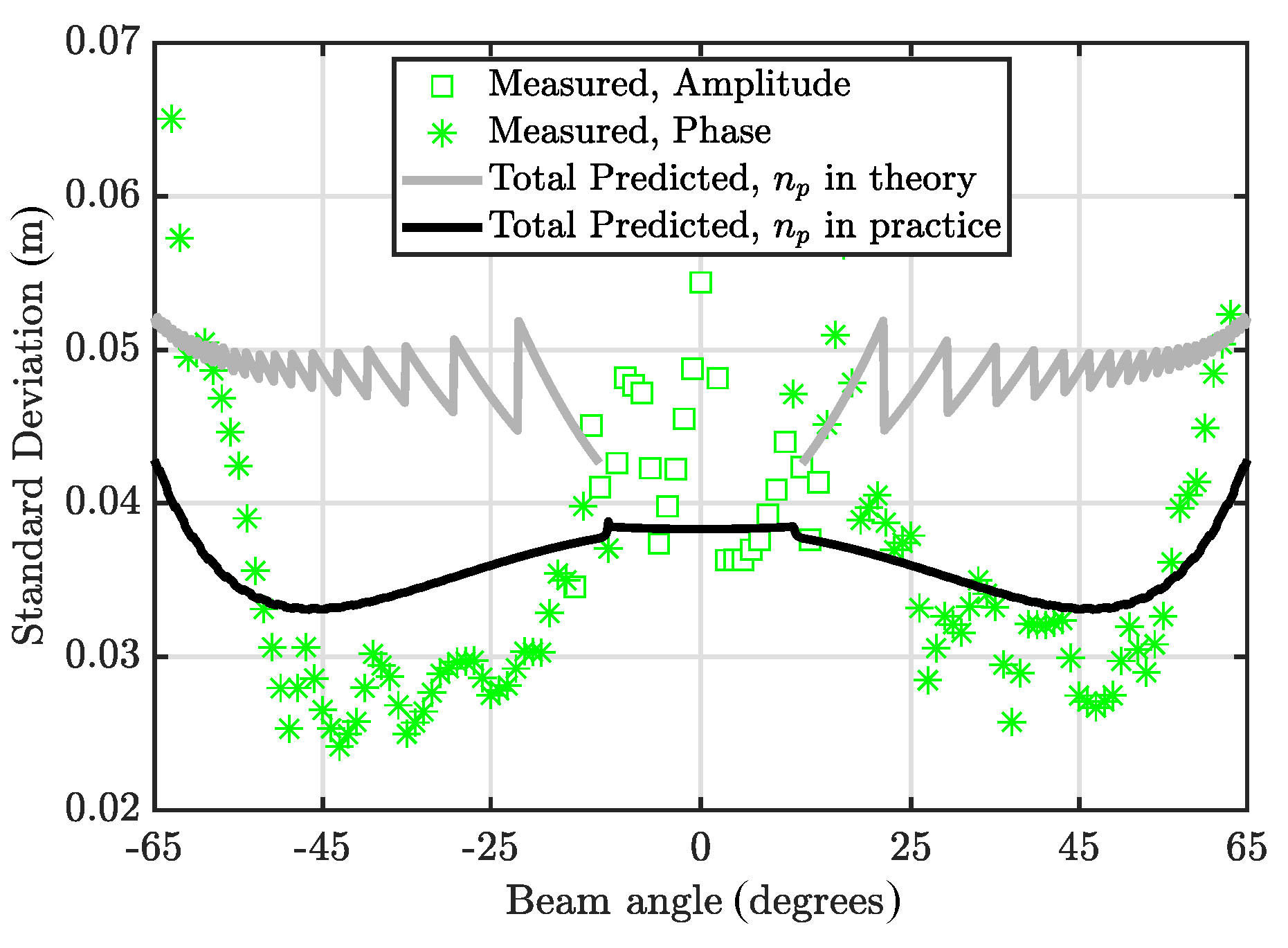
Generally, information regarding the majority of the input parameters is reliable. However, in the expression used for predicting the bathymetric uncertainty due to the uncertainty in the phase bottom detection, the number of phase samples, , is used [6,7]. This was given in [40] as:
where indicates the angle between the received beam and nadir (depth-axis) [22]. is the across-track beam opening angle (the beam opening angle at reception), which increases with an increasing steering angle for the outer beams; see Table 1 for its value at nadir. How well this equation represents the actual number of phase samples is questionable as there is no information with regard to the approach taken by Kongsberg for deriving the number of phase samples per beam. Presented in Figure 4 with gray is the prediction of the bathymetric uncertainty for the situation in which the number of phase samples within the beam footprint was derived using Equation (5). Shown with black and green are the bathymetric uncertainties obtained using the number of phase samples extracted from the data [41] and those measured respectively. It is seen that in case of using the theoretical number of phase samples in the uncertainty prediction model, large discrepancies occurred between the modeled and measured uncertainties; compare the gray and green in Figure 4, in particular for the middle sector of the swath with the prediction overestimating the measured uncertainties. Using the number of phase samples obtained in practice for predicting the bathymetric uncertainties reduced this discrepancy to a noticeable extent. Therefore, for the comparison between the modeled and measured bathymetric uncertainties, the number of phase samples obtained in practice was used in the prediction model.
Shown in Figure 5 are the modeled and measured bathymetric uncertainties for the area indicated by the black dashed rectangle in Figure 1e for a water depth of 10 with a pulse length of 27 (a), 54 (b), and 134 (c). It should be noted that for the bottom detection method (amplitude or phase), the approach documented in the data was taken.
Both the measured and predicted depth uncertainties increase with increasing pulse length. In general, the uncertainties derived from the prediction model are in a good agreement with those encountered in reality with larger discrepancies occurring for the beams where the amplitude detection was used. The measured bathymetric uncertainty slightly increases with an increasing beam angle which is captured by the prediction model.
As discussed in Section 4.1, lengthening the pulse duration results in using the amplitude detection for a larger range of beams around nadir, and consequently, the model underestimates the bathymetric uncertainties for a broader range of beams; compare Figure 5a and Figure 5c. The most dominant source of uncertainty has been predicted to be the echosounder contribution; see the solid back line with circle markers. As discussed in Section 2.1, this contribution is divided into three terms (see [22,25]):
- Uncertainties in the range measurements,
- Uncertainties in the angle of impact of the incoming sound wave with the MBES,
- non-zero along-track beam opening angle.
The first and third contributions are equal for both amplitude and phase detection. However, the expression for the second term differs. In the case of using amplitude detection, the contribution of the across-track angular measurements’ uncertainty to the depth uncertainty is a constant term equaling [6,7]. Comparing the measured and predicted uncertainties suggested that this term requires modification.
An additional point to clarify is the term referred to as range sampling resolution used to calculate the contribution of the range measurements to the bathymetric uncertainty. This term is defined as with the sampling frequency. The reported value for is the output sampling frequency, different from the one used for applying the bandpass filters and beamforming with the latter being higher. Knowledge of this value is required for correct calculation of the contribution of the range measurements to the bathymetric uncertainty. If the sampling frequency used for the bottom detection would be in the order of , the contribution of the range error would become negligible. For the present contribution, lacking information on the sampling frequency of relevance, the maximum output sample rate of EM2040c equaling 60 was used for the predictions, corresponding to a contribution varying from at nadir to for the most outer beam to the bathymetric uncertainty.
Shown in Figure 6 are the modeled and measured depth uncertainties for the area indicated by the dashed line in Figure 1f for a water depth of 30 and pulse lengths of 27 (a), 54 (b), and 134 (c). Compared to the shallower water depth, for the two pulse lengths of 27 and 54 , the discrepancy between the modeled and measured uncertainties increases. This can partly indicate that the prediction model cannot fully capture the depth dependency of the bathymetric uncertainties. For the pulse with the longest duration, relatively good agreement is obtained between the predicted and measured uncertainties for the middle sector of the beams. With regards to the variations of the bathymetric uncertainty with the beam angle, in contrast to the data acquired at a water depth of 10 , the measured uncertainties show a pronounced dependency on the beam angle. This behavior is captured to a limited extent by the prediction model.
4.3. Improving Model-Data Agreement by Accounting for the Most Recent Insights into the Contributors to MBES Depth Uncertainties
In order to improve the agreement between the predicted and measured uncertainties, in particular for deeper waters, the contribution of the following uncertainty sources is added to the existing bathymetric uncertainty prediction model:
- Doppler effect: Since the MBES is constantly moving, the received signal is affected by a Doppler frequency shift. This frequency shift has an impact on the beam steering, resulting in uncertainties in the steering angle. An uncertainty in the steering angle gives rise to uncertainty in the estimated depths. As such, an underestimation of the contribution of the Doppler effect potentially leads to an optimistic expectation of the depth uncertainties; see [21]. This contribution increases with water depth and beam angle.
- Baseline decorrelation: As shown by Mohammadloo et al. [21], the phenomenon of baseline decorrelation occurs in the MBES interferometry step for phase detection due to slightly different received signals by the two sub-arrays resulting from different angular directions. Thus, the coherence between the two received signals is affected. As the water depth increases, this coherence is reduced (due to a larger signal footprint and consequently a more fluctuating directivity pattern), and thus, the quality of the phase estimates is negatively, affected resulting in an increase in the bathymetric uncertainty.
The current expressions used for the depth uncertainty prediction has not accounted for the contribution of the Doppler effect. However, the baseline decorrelation has been accounted for in an approximate way, not accounting for the specific pulse characteristics [21]. Here, it will be investigated to what extent these two factors modify the model-data agreement for the cases considered.
As discussed by Mohammadloo et al. [21], accounting for the contribution of the Doppler effect requires knowledge of the speed of the array center at emission and reception of the signal projected in the beam direction and the weather condition during the data acquisition. The weather condition during the survey was calm, and the same vessel and MBES as used in Mohammadloo et al. [21] were employed. We thus made use of the values derived by them for the calm weather condition; see Figure 3 in [21].
To quantify the effect of baseline decorrelation on MBES bathymetric measurements in the interferometry step, the standard deviation of the phase difference needs to be calculated [42]. The parameters required for this calculation are the actual pulse shape of the transmitted signal (the CW pulse shape used here with the center frequency presented in Table 1) and the length of each sub-array used in the interferometry step, equaling for the case considered, i.e., one-third of the theoretical array length corrected for the shading.
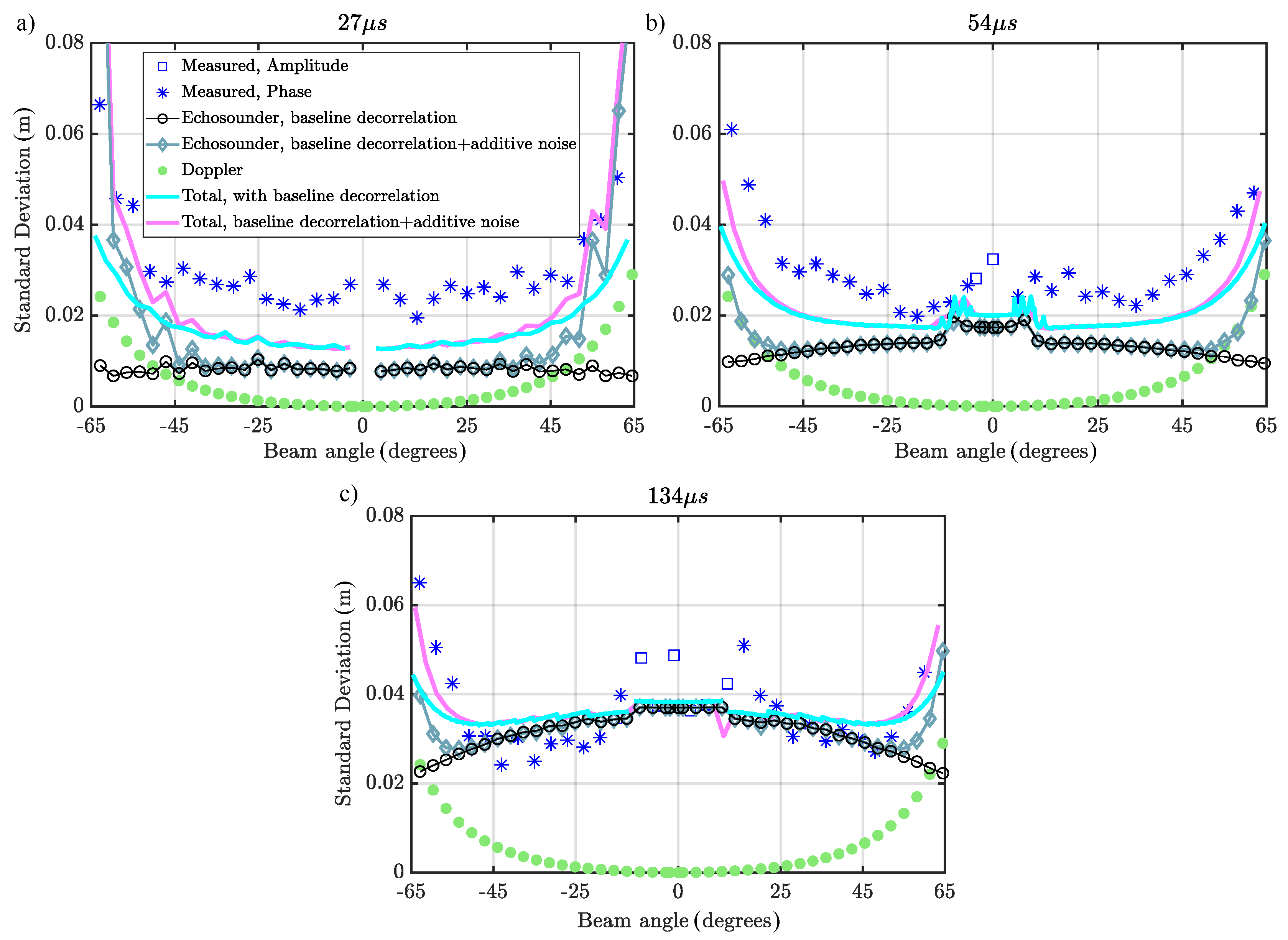
Shown in Figure 7 and Figure 8 are the measured and predicted depth uncertainties for a water depth of 10 and 30 , respectively, with varying pulse lengths where both the Doppler effect (light green circles) and baseline decorrelation are considered. The baseline decorrelation has now been considered within the echosounder contribution (solid black line with circle markers). The depth uncertainty induced by the motion sensor, correction accuracy for misalignment, sound speed, and heave were equal to those of Figure 5 and Figure 6 and are thus not shown here.
From Figure 7, it is seen that the contribution of the echosounder decreases with an increasing beam angle (as the coherence between the two received signal increases with an increasing beam angle), in contrast to Figure 5, where an increase in the uncertainty with the beam angle was observed. This indicates that accounting for the baseline decorrelation in the approximate way as carried out in [6,7] overestimates the uncertainties. It is also seen that although the total bathymetric uncertainty (cyan) decreases, the magnitude of the reduction is lower than that of the echosounder contribution, which is due to the compensation of the decrease by an increasing contribution of the Doppler effect with the beam angle. Compared to the situation where these contributions were not considered, the variations of the bathymetric uncertainty with the beam angle as seen in the measurements are captured better (compare the solid cyan curve corresponding to the total predicted uncertainty in this figure to that of Figure 5).
Furthermore, for the 30 water depth, a decrease in the contribution of the echosounder is observed (see Figure 8). With regard to the total bathymetric uncertainty, in contrast to the shallower depth where a decrease was seen, here, no noticeable change is observed except for the pulse length of 54 where an increase occurred. The almost equal uncertainties (compare Figure 6 and Figure 8) means that the decrease in the contribution of the echosounder is canceled out by the increase in the contribution of the Doppler effect. Compared to the measured uncertainties, still an underestimation occurs; however, accounting for the Doppler effect and baseline decorrelation can improve the performance of the uncertainty prediction model in capturing the increase of the measured uncertainties with the beam angle; see Figure 8b.
Although accounting for the baseline decorrelation and Doppler effect improved the performance of the prediction model in capturing the dependency of the depth uncertainties to the beam angle, still discrepancies between the predicted and measured vertical uncertainties remained. A potential contributor deteriorating the quality of the bathymetric measurements toward the outer parts of the swath is the decreased SNR, due to the additive noise [21,43]. The uncertainty prediction model assumes an infinite SNR, which is violated in reality. Here, we will investigate to what extent the additive noise contribution modifies the vertical uncertainty predictions for the cases considered. The SNR expresses the relative importance of the contribution of the expected received echo level and the perturbing noise and is given by the sonar equation [44]. The nature of the additive noise makes its prediction complicated as it requires information on the backscatter strength returned to the MBES, which is dependent on the composition of the seabed, angle of incidence, acoustic frequency, seafloor roughness, volume heterogeneity, and bulk density [45]. The backscatter strength received is the result of a complex interaction of the transmitted acoustic signal and the often inhomogeneous seafloor [46,47]. Here, the total backscatter strength was modeled as the result of a contribution from volume backscattering and rough interface backscattering based on the APL -model [48]. A priori knowledge of the surveyed areas indicated a very soft sediment, and thus, clayey sand was assumed in the APL-model. Indeed, the need for information on the sediment composition makes the prediction of the contribution of the additive noise complicated as such information might not be always available. For the calculation of the SNR, the transmitted source level also needed to be known. Here, this was assumed to be 20 dB lower than the maximum power available at the transmission (Kjetil Jensen, Kongsberg personal communication, June 2018). The transmission loss, the noise level, or the reverberation level inside the receiver band, the transmission and reception directivity patterns, the sensitivity of the transducer with respect to center frequency, and the receiver gain applied by the receiver electronics are other parameters required for the calculation of the SNR. The joint impact of the SNR and baseline decorrelation was then derived following Vincent [43]. Added to Figure 7 and Figure 8 with solid light blue lines with diamond markers and solid light pink lines are the echosounder contribution accounting for the uncertainties induced by the baseline decorrelation and additive noise and the resulting total depth uncertainty, respectively.
For a water depth of 10 , compared to the situation where the contribution of additive noise was discarded, no noticeable change is observed for the inner and middle sector of the beams, i.e., this means that the prediction model still (slightly) underestimates the measured uncertainties. However, as expected from the nature of the additive noise, the predicted depth uncertainty for the outer beams increased. This increase improved the ability of the prediction model in capturing the variation of the bathymetric uncertainty with the beam angle. Regarding the longest pulse length, a slight over-prediction occurs when accounting for the additive noise contribution.
As for the deeper surveyed area and the two shorter pulse lengths in Figure 8a,b, although still an underestimation occurs for the inner and middle beam sector, the increase of the bathymetric uncertainties with increasing beam angle is now well predicted. As for the longest pulse length, a very good agreement between the modeled and measured depth uncertainties is obtained for all the beam angles, which was expected as the discrepancy observed between them discarding the contribution of the additive noise was mainly concerned with the most outer beams.
5. Conclusions
Predicting the uncertainty of MBES bathymetric measurements is an important and almost standard step in the planning of MBES surveys. Models have been developed to fulfil such a purpose enabling one to assess whether the required survey standards can be met in a specific measurement campaign for a given combination of measurement equipment, MBES, and environmental settings. Since the development of the these models, the MBES systems have been significantly improved. Moreover, new insights into the uncertainty sources affecting the quality of depth measurements have been obtained, such as the contribution of the baseline decorrelation, Doppler effect, and additive noise.
This paper focused on assessing the performance of the widely used bathymetric uncertainty prediction model by comparing the predicted uncertainties to those measured using different pulse lengths and water depths. To obtain the measured bathymetric uncertainties such that a fair comparison could be made with those modeled, a number of issues were found of importance as follows:
- The size of the bottom surface patches, used for the calculation of the measured bathymetric uncertainty accounting for the potential presence of the small-scale depth variations, has to be chosen carefully. If a too large surface patch is used, the bottom morphology might change within a patch to an extent that cannot be captured by the fitting process. Therefore, the derived bathymetric uncertainty does not solely depend on the uncertainties inherent to the MBES. On the other hand, if a too small surface patch is used, the number of soundings within a patch might not be enough to to give a robust estimate of the required statistics. The optimal size of the surface patch varies with water depth and was found by comparing the bathymetric uncertainty corresponding to different patch sizes.
- The number of phase samples within each beam is required for the calculation of the bathymetric uncertainty induced due to the phase bottom detection technique. The comparison between the theoretical number of samples and those obtained in practice revealed large discrepancies, and thus, the latter was used for a realistic comparison between the measured and predicted bathymetric uncertainties.
Based on the comparison between the measured and predicted uncertainties, the following conclusions could be drawn:
- In general, the magnitude of the bathymetric uncertainties derived from the prediction model were in good agreement with those measured. However, discrepancies were observed with increasing water depth and for the outer beams.
- The model tends to underestimate the measured uncertainties for the beams where the amplitude detection was used as the bottom detection method. As the pulse length increases, a larger range of beam angles around nadir uses this bottom detection method, and hence, the underestimation occurs for a wider portion of the swath.
- The most dominant contributor to the depth uncertainty was found to be the echosounder contribution, and hence, as a first step toward improving the model, the contributions of the baseline decorrelation and Doppler effect were added to this contribution. The comparison between the situations with and without accounting for these error sources indicated a decrease in the contribution of the echosounder in the case of the former. The effect on the total bathymetric uncertainty depended also on the magnitude of the Doppler effect (as the reduction in the contribution of the baseline decorrelation with the beam angle was counteracted by an increase in the Doppler induced depth uncertainty).
- Accounting for the contributions of the Doppler effect and baseline decorrelation in general improves the performance of the prediction model in capturing the variations of the uncertainty with the beam angle. The agreement between the modeled and measured uncertainties for the outer parts of the swath is further improved by accounting for the decreased SNR. Accounting for these considerations, however, requires knowledge of the pulse shape, speed of the array at reception, and transmission of the signal and sediment characteristics, which might not be always available.
- Based on the insights obtained by accounting for the contribution of the baseline decorrelation and Doppler effect, one can conclude that the good model-data agreement obtained without accounting for these contributions might have been a coincidence. This occurred as a consequence of accounting for the baseline decorrelation in an approximate manner and discarding the contribution of the Doppler effect; for the situations considered here, it was found that the contributions of the baseline decorrelation when accounting for the pulse shape and Doppler effect counteracted each other. However, for a different environmental condition, survey configuration, or pulse shape, this might not occur. Consequently, not accounting for these contributions in the uncertainty prediction model can lead to incorrect predictions.
- Overall, this paper showed that the current capabilities of modeling the MBES bathymetric uncertainties in a computationally efficient way (error propagation) provided estimates that were in good agreement with those obtained experimentally.
Author Contributions
Conceptualization, T.H.M.; data curation, T.H.M.; methodology, T.H.M. and M.S.; software, T.H.M.; investigation, T.H.M.; writing, original draft preparation, T.H.M.; writing, review and editing, T.H.M., M.S., and D.G.S.; visualization, T.H.M.; supervision, M.S. and D.G.S.; funding acquisition M.S. and D.G.S. All authors read and agreed to the published version of the manuscript
Funding
This investigation is part of research funded by the Ministry of Infrastructure and Water management of The Netherlands, Rijkswaterstaat, The Netherlands.
Acknowledgments
The authors would like to thank the Ministry of Infrastructure and Water Management of the Netherlands (Rijkswaterstaat) for data acquisition and for providing measurements equipment. The authors would like to specifically thank Simon Bicknese for supporting the data acquisition.
Conflicts of Interest
The authors declare no conflict of interest.
References
- Komatsu, T.; Igarashi, C.; Tatsukawa, K.; Sultana, S.; Matsuoka, Y.; Harada, S. Use of multi-beam sonar to map seagrass beds in Otsuchi Bay on the Sanriku Coast of Japan. Aquat. Living Resour. 2003, 16, 223–230. [Google Scholar] [CrossRef]
- Anderson, T.J.; Syms, C.; Roberts, D.A.; Howard, D.F. Multi-scale fish-habitat associations and the use of habitat surrogates to predict the organisation and abundance of deep-water fish assemblages. J. Exp. Mar. Biol. Ecol. 2009, 379, 34–42. [Google Scholar] [CrossRef]
- Di Maida, G.; Tomasello, A.; Luzzu, F.; Scannavino, A.; Pirrotta, M.; Orestano, C.; Calvo, S. Discriminating between Posidonia oceanica meadows and sand substratum using multibeam sonar. ICES J. Mar. Sci. 2011, 68, 12–19. [Google Scholar] [CrossRef] [Green Version]
- Lurton, X.; Augustin, J.M. A measurement quality factor for swath bathymetry sounders. IEEE J. Ocean. Eng. 2010, 35, 852–862. [Google Scholar] [CrossRef]
- Hellequin, L.; Boucher, J.M.; Lurton, X. Processing of high-frequency multibeam echo sounder data for seafloor characterization. IEEE J. Ocean. Eng. 2003, 28, 78–89. [Google Scholar] [CrossRef] [Green Version]
- Hare, R. Depth and position error budgets for multibeam echosounding. Int. Hydrogr. Rev. 2003, LXXII, 37–69. [Google Scholar]
- Hare, R. Error Budget Analysis for US Naval Oceanographic Office (NAVOCEANO) Hydrographic Survey Systems; Technical Report; Hydrographic Science Research Center (HSRC): Hattiesburg, MS, USA, 2001. [Google Scholar]
- Calder, B.R.; Mayer, L.A. Robust Automatic Multi-beam Bathymetric Processing. In Proceedings of the U.S. Hydrographic Conference, Norfolk, VA, USA, 21–24 May 2001; pp. 1–20. [Google Scholar]
- Calder, B.R.; Mayer, L.A. Automatic processing of high-rate, high-density multibeam echosounder data. Geochem. Geophys. Geosyst. 2003, 4. [Google Scholar] [CrossRef]
- Calder, B.R. Distribution-free, Variable Resolution Depth Estimation with Composite Uncertainty. In Proceedings of the U.S. Hydrographic Conference, New Orleans, LA, USA, 25–27 March 2013; pp. 1–8. [Google Scholar]
- Eakins, B.W.; Taylor, L.A. Seamlessly Integrating Bathymetric and Topographic Data to Support Tsunami Modeling and Forecasting Efforts. In Ocean Globe; Esri Press: Redlands, CA, USA, 2010; Chapter 2; pp. 37–56. [Google Scholar]
- Hare, R.; Eakins, B.W.; Amante, C.; Taylor, L.A. Modeling bathymetric uncertainty. Int. Hydrogr. Rev. 2011, 6, 31–42. [Google Scholar]
- Lundblad, E.R.; Wright, D.J.; Miller, J.; Larkin, E.M.; Rinehart, R.; Naar, D.F.; Donahue, B.T.; Anderson, S.M.; Battista, T. A benthic terrain classification scheme for American Samoa. Mar. Geod. 2006, 29, 89–111. [Google Scholar] [CrossRef] [Green Version]
- Wilson, M.F.J.; O’Connell, B.; Brown, C.; Guinan, J.C.; Grehan, A.J. Multiscale terrain analysis of multibeam bathymetry data for habitat mapping on the continental slope. Mar. Geod. 2007, 30, 3–35. [Google Scholar] [CrossRef] [Green Version]
- Eleftherakis, D.; Amiri-Simkooei, A.; Snellen, M.; Simons, D.G. Improving riverbed sediment classification using backscatter and depth residual features of multi-beam echo-sounder systems. J. Acoust. Soc. Am. 2012, 131, 3710–3725. [Google Scholar] [CrossRef] [Green Version]
- Eleftherakis, D.; Snellen, M.; Amiri-Simkooei, A.; Simons, D.G.; Siemes, K. Observations regarding coarse sediment classification based on multi-beam echo-sounder’s backscatter strength and depth residuals in Dutch rivers. J. Acoust. Soc. Am. 2014, 135, 3305–3315. [Google Scholar] [CrossRef] [Green Version]
- Snellen, M.; Gaida, T.C.; Koop, L.; Alevizos, E.; Simons, D.G. Performance of multibeam echosounder backscatter-based classification for monitoring sediment distributions using multitemporal large-scale ocean datasets. IEEE J. Ocean. Eng. 2018, 44, 142–155. [Google Scholar] [CrossRef] [Green Version]
- Gaida, T.C.; Mohammadloo, T.H.; Snellen, M.; Simons, D.G. Mapping the seabed and shallow subsurface with multi-frequency multibeam echosounders. Remote Sens. 2020, 12, 52. [Google Scholar] [CrossRef] [Green Version]
- Kongsberg Maritime. EM Technical Note: Filters and Gains for EM 2040, EM 710, EM 302 and EM 122. 2017. Available online: https://www.kongsberg.com/globalassets/maritime/km-products/product-documents/kongsberg-em-technical-note-em-runtime-parameters-filters-and-gains-basic.pdf (accessed on 6 July 2020).
- Kongsberg Maritime. EM Technical Note: Advanced Filters and Gains for EM 2040, EM 710, EM 302 and EM 122. 2017. Available online: https://www.kongsberg.com/globalassets/maritime/km-products/product-documents/kongsberg-em-technical-note-em-runtime-parameters-filters-and-gains-advanced.pdf (accessed on 6 July 2020).
- Mohammadloo, T.H.; Snellen, M.; Simons, D.G. Multi-beam echo-sounder bathymetric measurements: Implications of using frequency modulated pulses. J. Acoust. Soc. Am. 2018, 144, 842–860. [Google Scholar] [CrossRef] [PubMed] [Green Version]
- Mohammadloo, T.H.; Snellen, M.; Amiri-Simkooei, A.; Simons, D.G. Comparing Modeled and Measured Bathymetric Uncertainties: Effect of Doppler and Baseline Decorrelation. In Proceedings of the OCEANS 2019, Marseille, France, 17–20 June 2019; pp. 1–8. [Google Scholar]
- Maleika, W. The influence of track configuration and multibeam echosounder parameters on the accuracy of seabed DTMs obtained in shallow water. Earth Sci. Inform. 2013, 6, 47–69. [Google Scholar] [CrossRef]
- Mohammadloo, T.H.; Snellen, M.; Simons, D.G.; Dierikx, B.; Bicknese, S. Using alternatives to determine the shallowest depth for bathymetric charting: Case study. J. Surv. Eng. 2019, 145, 05019004. [Google Scholar] [CrossRef] [Green Version]
- Mohammadloo, T.H.; Snellen, M.; Amiri-Simkooei, A.; Simons, D.G. Assessment of Reliability of Multi-beam Echo-sounder Bathymetric Uncertainty Prediction Models. In Proceedings of the 5th Underwater Acoustics Conference and Exhibition, Crete, Greece, 30 June–5 July 2019; pp. 783–790. [Google Scholar]
- Ladroit, Y.; Lurton, X.; Sintès, C.; Augustin, J.; Garello, R. Definition and Application of a Quality Estimator for Multibeam Echosounders. In Proceedings of the 2012 Oceans—Yeosu, Yeosu, Korea, 21–24 May 2012; pp. 1–7. [Google Scholar]
- Amiri-Simkooei, A.; Snellen, M.; Simons, D.G. Riverbed sediment classification using multi-beam echo-sounder backscatter data. J. Acoust. Soc. Am. 2009, 126, 1724–1738. [Google Scholar] [CrossRef]
- Teunissen, P.J.G.; Simons, D.G.; Tiberius, C.C.J.M. Probability and Observation Theory: An Introduction; Lecture Notes AE2-E01; Faculty of Aerospace Engineering, Delft University of Technology, Delft University: Delft, The Netherlands, 2006. [Google Scholar]
- Kongsberg Maritime. EM2040C MKII. 2019. Available online: https://www.kongsberg.com/globalassets/maritime/km-products/product-documents/em-2040c-compact-multibeam-echosounder.pdf (accessed on 6 July 2020).
- Kongsberg Maritime. EM Technical Note: Sector Coverage and Beam Spacing Modes for Multibeam Echosounders. 2019. Available online: https://www.kongsberg.com/globalassets/maritime/km-products/product-documents/em-sector-coverage-beam-spacing-modes.pdf (accessed on 6 July 2020).
- National Oceanic and Atmospheric Administration. Hydrographic Survey Specifications and Deliverables; Technical Report; U.S. Department of Commerce, National Oceanic and Atmospheric Administration: Washington, DC, USA, 2018. Available online: https://nauticalcharts.noaa.gov/publications/docs/standards-and-requirements/specs/hssd-2018.pdf (accessed on 6 July 2020).
- AML Oceanographic. SV & CTD Profilers: Base.X2 and Minos.X. 2016. Available online: http://www.mdsys.co.kr/down/AML/Base%20X2.pdf (accessed on 6 July 2020).
- QINSy. How-to Height—Tide and RTK. 2020. Available online: https://confluence.qps.nl/qinsy/9.0/en/how-to-height-tide-and-rtk-128680602.html (accessed on 6 July 2020).
- iXblue. Phins Subsea: FOG-Based High-Performance Inertial Navigation System. 2020. Available online: https://www.ixblue.com/sites/default/files/2019-10/PhinsSubsea_2019.pdf (accessed on 6 July 2020).
- Godin, A. The Calibration of Shallow Water Multibean Echo-Sounding Systems. Master’s Thesis, Department of Geodesy and Geomatics Engineering, University of New Brunswick, Fredericton, NB, Canada, 1998. [Google Scholar]
- Hughes Clarke, J.E. Dynamic motion residuals in swath sonar data: Ironing out the creases. Int. Hydrogr. Rev. 2003, 4, 6–23. [Google Scholar]
- Herlihy, D.; Hillard, B.; Rulon, T. National oceanic and atmospheric administration SEA BEAM system “patch test”. Int. Hydrogr. Rev. 1989, LXVI, 119–139. [Google Scholar]
- Mohammadloo, T.H.; Snellen, M.; Renoud, W.; Beaudoin, J.D.; Simons, D.G. Correcting multibeam echosounder bathymetric measurements for errors induced by inaccurate water column sound speeds. IEEE Access 2019, 7, 122052–122068. [Google Scholar] [CrossRef]
- Burdic, W.S. Underwater Acoustic System Analysis, 2nd ed.; Englewood Cliffs: Prentice-Hall, NJ, USA, 1991. [Google Scholar]
- Simons, D.G.; Snellen, M. A Bayesian approach to seafloor classification using multi-beam echo-sounder backscatter data. Appl. Acoust. 2009, 70, 1258–1268. [Google Scholar] [CrossRef]
- Kongsberg Maritime Instruction Manual: EM Series Multibeam Echo Sounder, Datagram Formats. 2015. Available online: http://www3.mbari.org/products/mbsystem/formatdoc/Kongsberg/EM_Datagram_Formats_RevS.pdf?OpenElement (accessed on 6 July 2020).
- Tough, J.A.; Balcknell, D.; Quegan, S. A statistical description of polarimetric and interferometric synthetic aperture radar data. Proc. R. Soc. Lond. A Math. Phys. Eng. Sci. 1995, 449, 567–589. [Google Scholar]
- Vincent, P. Modulated Signal Impact on Multibeam Echosounder Bathymetry. Ph.D. Thesis, Télécom Bretagne Sous En habilitation conjointe avec ĺUniversité de Rennes 1, Rennes, France, 2013. [Google Scholar]
- Urick, R.G. Principles of Underwater Sound, 3rd ed.; Peninsula Publishing: Westport, CT, USA, 1983. [Google Scholar]
- Jackson, D.R.; Richardson, M.D. High-Frequency Seafloor Acoustics; Springer: New York, NY, USA, 2006. [Google Scholar]
- Sternlicht, D.D.; de Moustier, C.P. Time-dependent seafloor acoustic backscatter (10–100 kHz). J. Acoust. Soc. Am. 2003, 114, 2709–2725. [Google Scholar] [CrossRef] [Green Version]
- Simons, D.G.; Snellen, M. A comparison between modeled and measured high frequency bottom backscattering. J. Acoust. Soc. Am. 2008, 123, 3895. [Google Scholar] [CrossRef] [Green Version]
- Applied Physics Laboratory, University of Washington. APL-UW High-Frequency Ocean Environmental Acoustic Models Handbook; Technical Report APL-UW TR9407; Applied Physics Laboratory, University of Washington: Seattle, WA, USA, 1994. [Google Scholar]
Figure 1.
Study areas: (a) the North Sea and (b) southwest of The Netherlands showing the Oosterschelde estuary (Eastern Scheldt) and the location of the two datasets. Bathymetry maps of the surveyed area for (c) a 10 water depth with the grid cell size of × , (d) a 30 water depth with the grid cell size of 1 × 1 , (e) zoomed in on the black rectangle shown in (c), and (f), and zoomed in on the black rectangle shown in (d). The bathymetry maps correspond to the measurements with a pulse length of 54 . The black rectangles in (e,f) indicate the areas considered for the depth uncertainty calculation.

Figure 2.
Mean value of the vertical uncertainty for different patch sizes in the across-track direction (squares with varying colors) for a water depth of 10 (gray line) and 30 (black line) and a pulse length of 54 .
Figure 2.
Mean value of the vertical uncertainty for different patch sizes in the across-track direction (squares with varying colors) for a water depth of 10 (gray line) and 30 (black line) and a pulse length of 54 .

Figure 3.
Standard deviation of the depth measurements for water depths of (a) 10 and (b) 30 , with a pulse length of 27 (red), 54 (green), and 134 (blue). The transition from the amplitude (Ampl) to phase (Ph) detection is shown by changing the square marker to an asterisk.
Figure 3.
Standard deviation of the depth measurements for water depths of (a) 10 and (b) 30 , with a pulse length of 27 (red), 54 (green), and 134 (blue). The transition from the amplitude (Ampl) to phase (Ph) detection is shown by changing the square marker to an asterisk.

Figure 4.
Predictions of total bathymetric uncertainty for a water depth of 30 and a pulse length of 134 using the number of phase samples obtained from Equation (5) (gray) and extracted from the data (black). Shown with green markers are the measured vertical uncertainties. The transition from the amplitude to phase detection is shown by changing the square marker to an asterisk.

Figure 5.
Bathymetric uncertainty derived from the measurements (blue markers) and those predicted for a water depth of 10 and a pulse length of (a) 27 , (b) 54 , and (c) 134 . The change from amplitude to phase detection is shown by switching from square markers to asterisks with the same color. The location of this switch was similarly applied in the modeling.

Figure 6.
Bathymetric uncertainty derived from the measurements (blue) and those predicted for a water depth of 30 and a pulse length of (a) 27 , (b) 54 , and (c) 134 . The change from amplitude to phase detection is shown by switching from square markers to asterisks with the same color. The location of this switch was similarly applied in the modeling.

Figure 7.
Bathymetric uncertainty derived from the measurements (blue) and those predicted considering the uncertainty induced by the Doppler effect and baseline decorrelation without (cyan) and with (light pink) additive noise for a water depth of 10 and a pulse length of (a) 27 , (b) 54 , and (c) 134 . The change from amplitude to phase detection is shown by switching from square markers to asterisks with the same color. The location of this switch was similarly applied in the modeling. The depth uncertainty induced by motion sensor measurements, correction accuracy for misalignment, sound speed, and heave are equal to those of Figure 5 and are thus not shown here.

Figure 8.
Bathymetric uncertainty derived from the measurements (blue) and those predicted considering the uncertainty induced by the Doppler effect and baseline decorrelation without (cyan) and with (light pink) additive noise for a water depth of 30 and a pulse length of (a) 27 , (b) 54 , and (c) 134 . The change from amplitude to phase detection is shown by switching from square markers to asterisks with the same color. The location of this switch was similarly applied in the modeling. The depth uncertainty induced by motion sensor measurements, correction accuracy for misalignment, sound speed, and heave are equal to those of Figure 6 and are thus not shown here.


Table 1.
Characteristics of EM2040C [29] in the dual head configuration.
Table 1.
Characteristics of EM2040C [29] in the dual head configuration.
| Parameter | Value |
|---|---|
| Center frequency ( ) | 300 |
| Theoretical array length ( ) | 0.407 |
| Number of beams (dual swath) (#) | 800 |
| Beam spacing mode | equiangular |
| Maximum swath width () | 130 |
| Mounting angle of transducer () | 39.89 for Starboard, 40.57 for Port |
| Beam steering reference angle () | 0 |
| Along-track opening angle () | 0.9 |
| Across-track opening angle at nadir () | 0.9 |
| Range resolution ( ) | 0.02525 |
© 2020 by the authors. Licensee MDPI, Basel, Switzerland. This article is an open access article distributed under the terms and conditions of the Creative Commons Attribution (CC BY) license (http://creativecommons.org/licenses/by/4.0/).
Share and Cite
MDPI and ACS Style
H. Mohammadloo, T.; Snellen, M.; G. Simons, D. Assessing the Performance of the Multi-Beam Echo-Sounder Bathymetric Uncertainty Prediction Model. Appl. Sci. 2020, 10, 4671. https://0-doi-org.brum.beds.ac.uk/10.3390/app10134671
AMA Style
H. Mohammadloo T, Snellen M, G. Simons D. Assessing the Performance of the Multi-Beam Echo-Sounder Bathymetric Uncertainty Prediction Model. Applied Sciences. 2020; 10(13):4671. https://0-doi-org.brum.beds.ac.uk/10.3390/app10134671
Chicago/Turabian StyleH. Mohammadloo, Tannaz, Mirjam Snellen, and Dick G. Simons. 2020. "Assessing the Performance of the Multi-Beam Echo-Sounder Bathymetric Uncertainty Prediction Model" Applied Sciences 10, no. 13: 4671. https://0-doi-org.brum.beds.ac.uk/10.3390/app10134671
Note that from the first issue of 2016, this journal uses article numbers instead of page numbers. See further details here.