Microfluidic Quantification of Blood Pressure and Compliance Properties Using Velocity Fields under Periodic On–Off Blood Flows

Abstract

To monitor variations of blood samples effectively, it is required to quantify static and dynamic properties simultaneously. With previous approaches, the viscosity and elasticity of blood samples are obtained for static and transient flows with two syringe pumps. In this study, simultaneous measurement of pressure and equivalent compliance is suggested by analyzing the velocity fields of blood flows, where a blood sample is delivered in a periodic on-off fashion with a single syringe pump. The microfluidic device is composed of a main channel (mc) for quantifying the equivalent compliance and a pressure channel (pc) for measuring the blood pressure. Based on the mathematical relation, blood pressure at junction (P_x) is expressed as P_x = kβ. Here, β is calculated by integrating the averaged velocity in the pressure channel (<U_pc>). The equivalent compliance (C_eq) is then quantified as C_eq = λ_off · Q₀/P_x with a discrete fluidic model. The time constant (λ_off ) is obtained from the transient behavior of the averaged blood velocity in the main channel (<U_mc>). According to results, P_x and C_eq varied considerably with respect to the hematocrit and flow rate. The present method (i.e., blood pressure, compliance) shows a strong correlation with the previous method (i.e., blood viscosity, elasticity). In conclusion, the present method can be considered as a potential tool for monitoring the mechanical properties of blood samples supplied periodically from a single syringe pump.

1. Introduction

As red blood cells (RBC) are the most common cells in blood, they have a strong influence on the mechanical properties of blood samples. Various mechanical properties of blood samples (i.e., blood viscoelasticity, RBC deformability, and RBC aggregation) have been used to monitor physical variations in blood samples. Blood viscosity is determined primarily by RBC aggregation at lower shear rates and by deformability at higher shear rates. Plasma proteins contribute to enhancing RBC aggregation. Owing to their unique features, such as high surface–volume (S–V) ratios, low cytoplasmic viscosities, and soft plasma membranes, RBCs can travel into micro-sized vessels that are smaller than their diameters. Hemoglobin, hydration, and ion pumps contribute to varying RBC flexibility and blood viscosity [1]. Altered membranes and cell functions in inherited RBC disorders exhibit decreases in RBC deformability. RBC deformability decreases due to altered RBC geometry, increased cytoplasmic viscosity, and altered membrane viscoelasticity [1]. Altered RBC mechanical properties are strongly correlated to various diseases, such as hereditary disorders, metabolic disorders, adenosine-triphosphate-induced membrane changes, oxidative stress, and paroxysmal nocturnal hemoglobinuria [2]. For these reasons, hemorheological properties have been stressed as potential indicators of specific pathological disorders. They are considered as label-free biomarkers for monitoring cell status and clinical relevance [2]. As blood samples flow dynamically through blood vessels (i.e., arteries, arterials, and capillaries), it is necessary to measure static property (i.e., viscosity or pressure) obtained under constant flow conditions and dynamic property (i.e., elasticity or compliance) obtained under transient flow conditions.

Using blood delivery tools (i.e., syringe pumps, pressure sources), blood samples can be supplied into a microfluidic device at a constant flow rate. Blood viscosity can then be obtained by means of several techniques (i.e., coflowing streams [3,4], reversal flow switching [5], advancing meniscus [6,7,8,9,10], electric impedance [11,12], droplet length [13], and digital flow compartment [14]). Among these methods, the parallel flow method has been used widely due to simplicity and continuous monitoring. It does not require a calibration procedure with standard fluid. However, the method requires two syringe pump to supply the blood sample and reference fluid. As syringe pumps are bulky and very expensive, it is necessary to reduce the number of syringe pumps. Furthermore, the previous method does not provide information on blood elasticity. More recently, the author has suggested the viscoelasticity measurement technique in dynamic varying flow conditions. First, by controlling the blood flow rate in the oscillatory pattern, the viscosity and elasticity can be obtained periodically by analyzing the interface in coflowing streams (i.e., blood stream, 1× phosphate-buffered saline (PBS) stream) [15]. Second, viscosity and elasticity can be obtained sequentially by monitoring reversal flow switching in a Wheatstone bridge circuit under a steady flow and transient flow. As a limitation, the previous methods require two pumps to supply two fluids.

Instead of blood viscosity, blood pressure is suggested to monitor the mechanical properties of blood samples, where blood samples are delivered into a microfluidic device with a single syringe pump. Burns et al. measured the liquid pressure inside the microfluidic channel by monitoring the air–liquid interface in the glass substrate [16]. To avoid air leakage throughout the polydimethylsiloxane (PDMS) polymer, the microfluidic device was fabricated with a glass substrate. Wu et al. measured liquid pressure with the same principle suggested by Burns et al. [17]. They used a glass capillary to monitor the liquid–air interface. Kaneko et al. reported that the local pressure inside a microfluidic device was monitored by analyzing the color intensity resulting from channel deformation [18]. Recently, blood pressure measurement has been demonstrated by monitoring the image intensity of RBCs collected in large channels (~2 × 22.5 mm²) [19]. To increase the sensitivity of blood pressure measurement, a polyethylene tubing can be connected to the outlet of the microfluidic device. After the channel is filled with high-density counter fluid, the outlet of the chamber is clamped completely with a pinch valve. As a drawback, the method requires a large channel to inspect the overall images of RBCs appropriately. To inspect cell-to-liquid interfaces in the chamber, the channel should be filled with counter fluid (i.e., glycerin) in advance. Because the shear rate is extremely low in the channel, RBC aggregation substantially contributes to the varying image intensity [20]. Thus, these methods should be improved to resolve these critical issues.

In this study, simultaneous quantification of blood pressure and equivalent compliance is demonstrated by obtaining velocity fields of blood samples flowing into a microfluidic-based compliance unit. Compared with previous methods, the proposed method provides two distinct advantages. First, the proposed method quantifies blood pressure by monitoring blood velocity inside the microfluidic-based compliant unit. Thus, it can be considered as one of the promising solutions for critical issues, such as the requirements for two-layer structures and the use of glass substrates or external tubing to avoid air leakage, large monitoring channels, and counter fluids. Second, by operating a single syringe pump in a periodic on–off fashion, two quantities (i.e., blood pressure and equivalent compliance) are obtained simultaneously and periodically. Thus, it is possible to monitor static and dynamic properties of blood samples with a single syringe pump.

2. Materials and Methods

2.1. Microfluidic Device and Experimental Setup

The microfluidic device used for measuring blood pressure and equivalent compliance of blood samples consisted of a main channel (mc) (width = 250 μm, length = 16.2 mm) and a pressure channel (pc) (width = 250 μm, length = 7.5 mm), as shown in Figure 1(A-a). The main channel contained inlet and outlet (a). The pressure channel was bifurcated at 7.6 mm from outlet (a) of the main channel. The pressure channel contained outlet (b). The channel depth of a microfluidic device was fixed at h = 10 μm. Conventional micro-electromechanical system techniques were used to fabricate a four inch silicon mold. Based on a soft lithography process with PDMS (Sylgard 184, Dow Corning, Midland, MI, USA) [15], a PDMS block was fabricated from the silicon mold. Using an oxygen plasma system, the PDMS block was bonded to the glass slide.

Polyethylene tubing (L₂) (length = 200 mm, inner diameter = 500 μm) was connected to outlet (a). Outlet (b) of the pressure channel was connected to polyethylene tubing (L₃) (length = 100 mm, inner diameter = 500 μm). After a disposable syringe (~1 mL) was filled with the blood sample (~0.5 mL), the needle of the syringe was fitted into the tubing (L₁). The disposable syringe was then installed into a syringe pump (neMESYS, Cetoni Gmbh, Germany). As shown in Figure 1(A-b), the syringe pump was positioned horizontally. The syringe pump was controlled in a periodic on–off fashion (i.e., period [T] = 480 s, duty ratio = 0.5, flow rate = Q₀). After filling both channels with the blood sample, the end of the tube (L₃) was clamped with a drawing pin. A microfluidic device was then positioned on an inverted microscope (BX51, Olympus, Tokyo, Japan). As shown in Figure 1(A-c), based on a high-speed camera (FASTCAM MINI, Photron, Tokyo, Japan), microscopic images were captured at a frame rate of 5000 frame per second (fps). Using an external trigger, two microscopic images were captured sequentially at intervals of 1 s. The camera offered a spatial resolution of 1280 × 1000 pixels. Each pixel corresponded to 10 μm.

2.2. Quantification of Velocity Fields in the Main Channel and Pressure Channel

First, to estimate the blood pressure at junction (P_x), it was necessary to obtain velocity fields of the blood sample flowing in the pressure channel. As shown in Figure 1B, a region-of-interest (ROI) with 150 × 250 pixels was selected within a pressure channel. By conducting micro particle image velocimetry (µPIV technique) [21], velocity fields across the pressure channel width (U_pc) were obtained over time. The size of the interrogation window was selected to be 64 × 64 pixels. The window overlap was set to 84%. The velocity fields were validated and corrected with a median filter. The averaged velocity (<U_pc>) was then calculated over the specific ROI.

Second, to estimate the time constant of the blood flow under transient blood flow, it was required to obtain velocity fields of the blood sample in the main channel. A specific ROI with 250 × 150 pixels was selected within the main channel. Velocity fields across the main channel width (U_mc) were obtained over time. The averaged velocity (<U_mc>) was calculated over the ROI.

2.3. Quantification of Blood Pressure and Compliance Properties

As a preliminary demonstration, the blood sample (normal RBCs in 1× PBS, Hct = 50%) was supplied into inlet with single syringe pump (i.e., T = 480 s, Q₀ = 1.5 mL/h).

Figure 1(C-a) shows a microscopic image captured at specific time (t = 0, 60, 120, 180, 240, 300, 360, and 420 s) during a single period. After turning on the syringe pump (Q₀ = 1.5 mL/h), the blood pressure at the junction increased over time. Then, the blood sample flowed forward in the pressure channel. After 60 s, the pressure reached equilibrium in the pressure channel. The RBCs then stopped moving forward over time. Because there was no existence of RBCs in the pressure channel, it was impossible to visualize blood flows. After turning off the syringe pump (Q₀ = 0), the blood pressure decreased over time. The blood sample flowed backwards for the remaining time of the period (240 s < t < 480 s). As the pressure channel was filled with the blood sample sufficiently, velocity fields of blood flows (U_pc) were obtained accurately with respect to time. Figure 1(C-b) shows temporal variations of <U_mc> and <U_pc> during the single period. Backward blood flow gave more consistent values of <U_pc> than forward blood flow. Thus, <U_pc> obtained under a backward blood flow was used to estimate pressure. Based on the mathematical formula of the compliance element, the pressure at junction (P_x) can be derived as:

$$P_x=\left(\frac{A_c}{C_f}\right)·\beta =k·\beta$$

(1)

In Equation (1), A_c and C_f mean the cross-sectional area and coefficient of compliance, respectively; β is expressed as Equation (2):

$$\beta ={\displaystyle \underset{0.5T}{\overset{T}{{\displaystyle \int }}}}\left|U_{pc}\right|dt$$

(2)

Because k = A_c/C_f has a constant value in Equation (1), pressure (P_x) was only determined by β. Here, a microfluidic system was modeled with discrete fluidic circuit elements, including the flow rate (Q_B, Q_m), resistance (R_c), and equivalent compliance (C_eq). Q_B and Q_m indicate the blood flow rate supplied from the syringe pump and the blood flow rate flowing in the main channel, respectively. R_c represents the fluidic resistance of the main channel filled with the blood sample. The fluidic resistance of the microfluidic channel (R_c) was much higher than that of the tubing (L₂) (R_t) connected to outlet (a) (i.e., R_c >> R_t). For this reason, R_c was only included in the fluidic circuit model. The equivalent compliance represents the summation of the tube compliance (C_t), channel compliance (C_c), and RBC compliance (C_RBCs) (i.e., C_eq = C_t + C_c + C_RBCs). Based on mass conservation at the junction (x), Equation (3) was derived as:

$$Q_B=\frac{P_x}{R_c}+C_{eq}\frac{d}{dt} \left(P_x\right)$$

(3)

In Equation (3), if P_x/R_c is replaced with Q_m (i.e., P_x/R_c = Q_m), Equation (1) can be simplified as:

$$R_c·C_{eq}·\frac{d}{dt} \left(Q_m\right)+Q_m=Q_B$$

(4)

Because Q_m is expressed as Q_m = A_c·<U_mc>, Equation (4) becomes Equation (5):

$${\lambda }_{off}\frac{d}{dt} \left(<U_{mc}>\right)+<U_{mc}>=\frac{Q_B}{A_c}$$

(5)

In Equation (5), the time constant (λ_off) is represented as λ_off = R_c·C_eq. Because P_x is expressed as P_x = R_c·Q₀, an equivalent compliance (C_eq) can be derived as:

C_eq = λ_off · Q₀/P_x

(6)

According to Equation (6), three factors (i.e., λ_off, Q₀, and P_x) were used to estimate equivalent compliance. As shown in Figure 1(C-b), using transient behaviors of <U_mc>, λ_off was obtained by conducting regression analysis with the model (i.e., <U_mc> = a₁ + a₂ exp (−t/λ_off)).

From the preliminary demonstration, it was estimated that two averaged velocities (<U_mc> and <U_pc>) could be effectively employed to estimate pressure and the equivalent compliance.

3. Results and Discussion

3.1. Contributions of Hematocrit, Flow Rate, and Diluent to Pressure and Equivalent Compliance

Before evaluating the performance of the present method, it was necessary to find out the contributions of several factors (hematocrit (Hct), flow rate (Q₀), diluent (1× PBS, plasma)) to blood pressure (P_x), and equivalent compliance (C_eq).

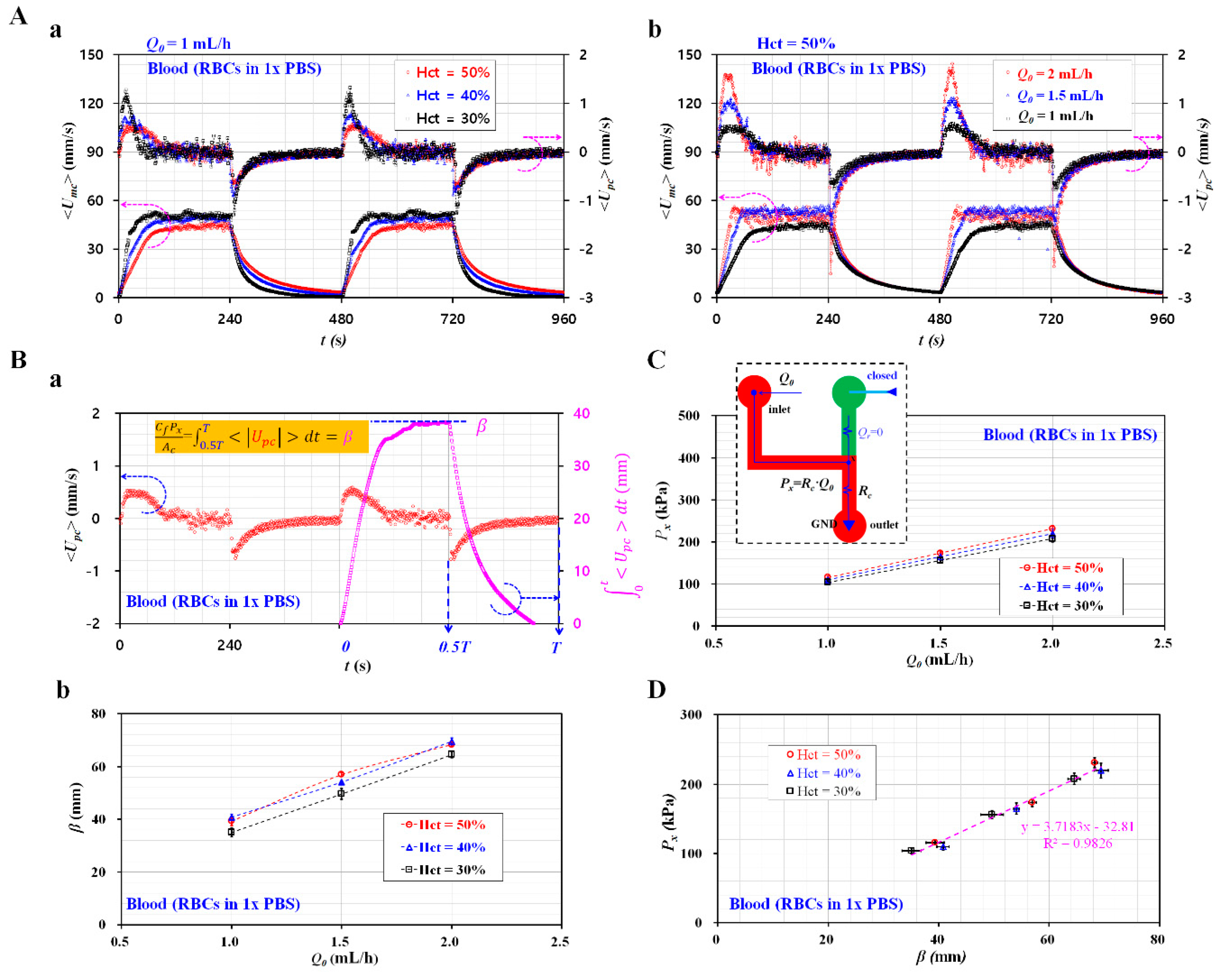
First, to evaluate the effects of Hct and Q₀ on <U_mc> and <U_pc>, temporal variations of <U_mc> and <U_pc> were obtained with respect to Hct = 30%, 40%, and 50%. Here, the diluent was fixed at 1× PBS. Blood sample preparation was discussed at the Section S1 (Supplementary Materials). The flow rate of the blood sample was fixed at Q₀ = 1 mL/h. According to an analytical formula for the depth of correlation (DOC) [22], the DOC was estimated as 64.1 µm. As the DOC was much higher than the channel depth (i.e., DOC >> depth), all RBCs contributed to calculation of the velocity fields of blood flows. Thus, the micro particle image velocimetry (μPIV) technique measured averaged velocity fields in the depth direction. As shown in Figure 2(A-a), both velocities tended to decrease substantially with respect to the hematocrit. To evaluate the contributions of Q₀ to <U_mc> and <U_pc>, temporal variations of both velocities were obtained with respect to Q₀ = 1, 1.5, and 2 mL/h. Here, the hematocrit was fixed at Hct = 50%. As shown in Figure 2(A-b), the peak time of <U_mc> tended to be short with respect to Q₀. Under transient flow conditions, <U_mc> could be employed to evaluate the effect of Q₀ on dynamic blood flows for up to Q₀ = 2 mL/h. Under a steady state condition, <U_mc> increased for up to Q₀ = 1.5 mL/h. Above Q₀ = 2 mL/h, <U_mc> did not increase significantly because the high-speed camera could not accurately capture the blood flow in the main channel. As <U_pc> was much lower than <U_mc>, there was no critical issue with consistent measurement of <U_pc> below Q₀ = 2 mL/h. Furthermore, <U_pc> increased considerably with respect to Q₀.

Second, to evaluate the contributions of Hct and Q₀ to pressure (P_x), temporal variations of <U_pc> were obtained, as shown in Figure 2(B-a). Using a mathematical formula of the compliance element, pressure at the junction was derived as $P_x=\frac{A_c}{C_f}{{\displaystyle \int }}_0^t<U_{pc}>dt$. Here, as shown in the right vertical axis of Figure 2(A-a), temporal variations of ${{\displaystyle \int }}_0^t<U_{pc}>dt$ were calculated by integrating <U_pc> over time. After turning on the syringe pump, <U_pc> showed transient behaviors. It arrived at a constant value (β) after 180 s. After turning off the syringe pump, <U_pc> decreased gradually over time from t = 0.5 T to t = T. It was assumed that the pressure was proportional to β. Because β was easily calculated from t = 0.5 T to t = T, β was defined as $\beta ={{\displaystyle \int }}_{0.5T}^T\left|U_{pc}\right|dt$. According to Equation (1), $P_x=k·\beta$, the unknown constant (k) was determined from experimental results. As shown in Figure 2A, using temporal variations of <U_pc>, variations of β were obtained with respect to Hct and Q₀. As shown in Figure 2(B-b), β tended to increase linearly. The hematocrit considerably contributed to increasing β. To find the relationship between β and P_x, the P_x was estimated approximately with a discrete fluidic circuit model. As shown in the inset of Figure 2C, the pressure channel was modeled by adding fluidic resistance and Q_r = 0, respectively. P_x was derived as P_x = R_c · Q₀ under a constant blood flow rate (Q₀). Because the fluidic resistance of the microfluidic channel (R_c) was much higher than that of the polyethylene tubing (R_t) (i.e., R_c >> R_t), R_c was only included in the fluidic circuit model. For a rectangular microfluidic channel with a low aspect ratio (i.e., depth (h)/width (w) = 10/250), R_c was approximated as $R_c=\frac{12{\mu }_{B}L}{w h^3}$, while μ_B and L represented blood viscosity and channel length. P_x was then expressed as $P_x=\frac{12{\mu }_{B}L}{w h^3}·Q_0$. Additionally, the shear rate ($\dot{\gamma }$) was estimated as $\dot{\gamma }=\frac{6Q_0}{w h^2}$. In a specific range of Q₀ = 1, 1.5, and 2 mL/h, it was estimated that the blood sample behaved as a Newtonian fluid because of $\dot{\gamma }>{10}^3{s}^{-1}$. According to coflowing streams reported in a previous study [3], the corresponding blood viscosity for each hematocrit was obtained as μ_B = 1.66 ± 0.06 cP for Hct = 30%, μ_B = 1.75 ± 0.09 cP for Hct = 40%, and μ_B = 1.85 ± 0.06 cP for Hct = 50%. As shown in Figure 2C, variations of P_x were obtained with respect to Hct and Q₀. Using a scatter plot, P_x and β were plotted on horizontal and vertical axes, respectively. To find out the proportional constant (k) between P_x and β, a linear regression analysis was conducted with EXCEL^TM (Microsoft, Redmond, Washington, WA, USA). As shown in Figure 2D, slope (k) was estimated as k = 3.1312 (R² = 0.9568). The result indicated that pressure could be obtained with P_x = 3.1312 β consistently.

Third, to evaluate the contributions of Hct and Q₀ to equivalent compliance (C_eq), the blood sample (normal RBCs suspended into 1× PBS) was supplied in a periodic on–off fashion (i.e., T = 480 s, Q₀ = 1, 1.5, and 2 mL/h). The hematocrit from blood sample was set to 30~50% within a physiological range. According to the Fahraeus effect, hematocrit distribution varies depending on narrow-sized channels (i.e., capillary mimicked channels). While blood samples flow in the microfluidic channels, hematocrit tends to decrease significantly when compared with hematocrit from the blood sample in the diving syringe.

As shown in Figure 3A, temporal variations of <U_mc> were obtained with respect to Hct = 30%, 40%, and 50%. As shown in Figure 3B, temporal variations of <U_mc> were obtained with respect to Hct and Q₀ = 1.5 mL/h. To find out λ_off, <U_mc> was assumed as <U_mc> = a₁ + a₂ exp (−t/λ_off). Here, the λ_off was obtained by conducting non-linear regression analysis with Matlab (version R2018a, Mathworks, Natick, MA, USA). The inset in Figure 3C shows a discrete fluidic circuit used to extract the time constant (λ_off) under transient blood flow. The velocity inside the pressure channel was much lower than the blood velocity in the main channel. Under periodic blood flow, the circuit model was modified by including Q_r = 0 and Q_C, whereby Q_C represented the flow rate in the compliance element. As shown in Figure 3C, variations of λ_off were obtained with respect to Q₀ and Hct. The λ_off remained unchanged with respect to Q₀. However, the time constant tended to increase with higher hematocrit levels. Based on Equation (6), variations of C_eq were obtained with respect to Hct and Q₀. As a result, C_eq tended to increase considerably with respect to Hct. However, Q₀ did not contribute to varying C_eq.

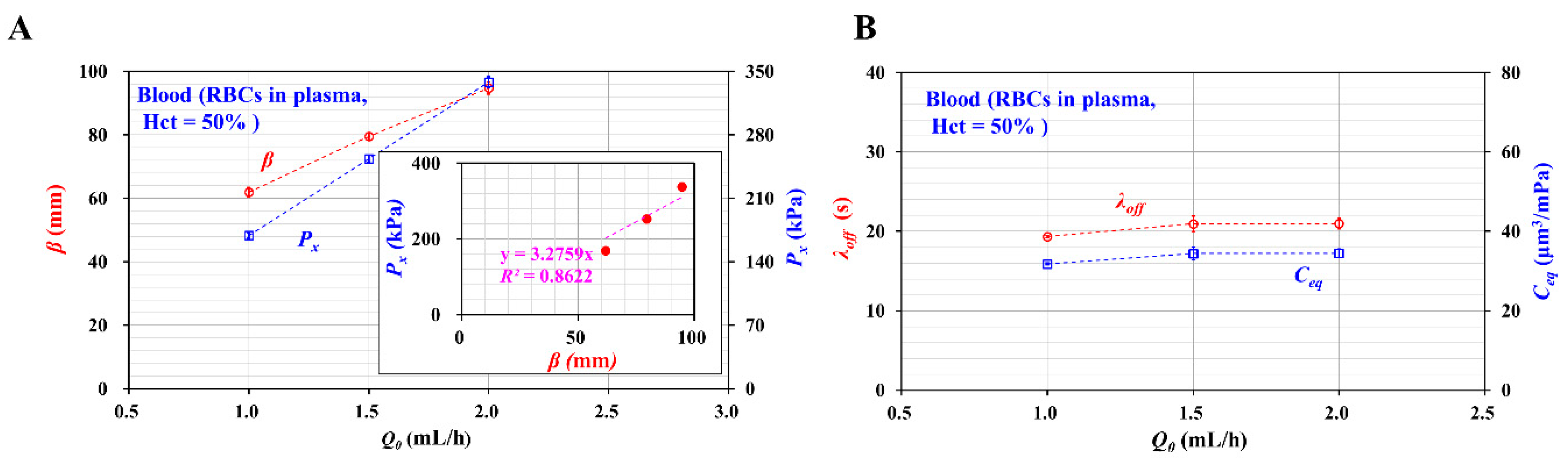
Finally, instead of using 1× PBS as the diluent, blood samples were adjusted to Hct = 50% by adding normal RBCs into plasma. Figure 4A shows variations of P_x and β with respect to Q₀. The inset of Figure 4A shows a linear relationship between P_x and β. According to the linear regression analysis, slope (k) was obtained as k = 3.2759. When compared with normal RBCs suspended into 1× PBS (i.e., k = 3.1312), the k of normal RBCs suspended in plasma showed a consistent value within a normalized difference range of 4.6%. Figure 4B shows variations of λ_off and C_eq with respect to Q₀. The λ_off and C_eq remained unchanged with respect to Q₀. When compared with the results shown in Figure 3C,D, both λ_off and C_eq tended to decrease with respect to Q₀.

From the results, the blood pressure at the junction (P_x) and the equivalent compliance (C_eq) varied significantly with respect to Hct and Q₀. For this reason, for consistent measurement of P_x and C_eq, Q₀ and Hct were fixed as Q₀ = 1.5 mL/h and Hct = 50% throughout all experiments. At the Section S2 (Supplementary Materials), contribution of erythrocyte sedimentation rate (ESR) in driving syringe to pressure and equivalent compliance were evaluated experimentally. In conclusion, blood pressure (P_x) did not provide consistent variations with respect to C_dex. Additionally, equivalent compliance (C_eq) gave constant values with respect to C_dex. However, as shown in Figure S1(A-b) (Supplementary Materials), the image intensity (<I_mc>) showed significant difference with respect to C_dex. For this reasons, to effectively quantify RBCs aggregation or ESR, the previous method (i.e., image intensity-based quantification) might be considered effective when compared with the present method (i.e., blood pressure or equivalent compliance).

3.2. Quantitative Comparison of the Present Method and Previous Method

To evaluate the performance of the present method, two quantities obtained at a constant flow rate and transient flow rate were compared with those obtained with the previous method. In other words, under a constant blood flow rate, pressure (P_x) obtained by the present method was compared with blood viscosity (μ_B) obtained by the previous method. Additionally, under the transient blood flow rate, the equivalent constant (C_eq) obtained by the present method was compared with the elasticity (G_B) obtained by the previous method [23].

First, blood pressure (P_x, present method) and blood viscosity (μ_B, previous method) were measured simultaneously for the same fixed blood sample. To vary the RBC deformability, normal RBCs were fixed chemically with various concentrations of glutaraldehyde (GA) solution (C_GA = 0, 2, 4, 6, 8, and 10 μL/mL). C_GA = 0 denoted 1× PBS as the diluent. The fixed blood sample (Hct = 50%) was prepared by adding homogeneous fixed RBCs into 1× PBS. As shown in Figure 5A, after setting the blood flow rate from Q₀ = 1.5 mL/h to Q₀ = 0, temporal variations of <U_pc> for a half period were obtained with respect to C_GA = 0, 6, and 10 μL/mL. Higher concentrations of the GA solution contributed to substantially increasing the magnitude of <U_pc>. Bases on Equations (1) and (2), variations of β and P_x were obtained with respect to C_GA. As shown in Figure 5B, β and P_x tended to increase distinctively with higher concentrations of the GA solution. The variations of β and P_x exhibited consistent trends because the GA solution contributed to stiffening the plasma membranes of the RBCs. When compared with the blood pressure obtained with the present method, blood viscosity for the same blood sample was quantified with coflowing streams, as in the previous method [4]. As shown in the inset of Figure 5C, the blood sample and the 1× PBS were supplied into a T-shaped channel at the same flow rate (i.e., Q_B = Q_PBS = 1.5 mL/h) with two syringe pumps. According to the coflowing method, blood viscosity (μ_B) was approximately derived as ${\mu }_B={\mu }_{PBS}·C_f·{\alpha }_B/\left(1-{\alpha }_B\right)$. To compensate for the model error resulting from difference in the boundary condition between the simple mathematical model and real physical model, the correction factor (C_f) was included as C_f = 1.4929 α_B⁴ −2.9858 α_B³ + 2.6301 α_B²−1.1372 α_B + 1.1971 (R² = 0.9874). Blood viscosity was then estimated by monitoring the blood-filled width (α_B). As shown in Figure 5C, the corresponding viscosity for each C_GA was obtained as μ_B = 1.427 ± 0.016 cP (C_GA = 0), μ_B = 1.485 ± 0.0.026 cP (C_GA = 2 μL/mL), μ_B = 1.499 ± 0.025 cP (C_GA = 4 μL/mL), μ_B = 1.611 ± 0.034 cP (C_GA = 6 μL/mL), μ_B = 2.071 ± 0.106 cP (C_GA = 8 μL/mL), and μ_B = 2.460 ± 0.1 cP (C_GA = 10 μL/mL). The results indicated that the blood viscosity increased substantially with respect to C_GA. As shown in Figure 5D, a scatter plot was used to observe the linear dependency between pressure (P_x, present method) and blood viscosity (μ_B, previous method). According to the linear regression analysis, R² had a sufficiently higher value (R² = 0.955). This result indicated that blood pressure was linearly proportional to blood viscosity (i.e., P_x = 71.195 μ_B + 65.621). For this reason, blood pressure could be effectively employed to monitor variations of blood samples instead of blood viscosity.

Second, under transient blood flow rates, equivalent compliance (C_eq, present method) and elasticity (G_B, previous method) were measured simultaneously for the same blood sample. As shown in Figure 6A, temporal variations of <U_mc> were obtained with respect to C_GA. At C_GA = 0 and 6 μL/mL, <U_mc> showed periodic variations over time consistently. However, at C_GA = 10 μL/mL, <U_mc> did not provide consistent variations at Q₀ = 1.5 mL/h. When the flow rate decreased from Q₀ = 1.5 mL/h to Q₀ = 0 (i.e., transient blood flow rate), <U_mc> showed consistent variations over time. The time constant (λ_off) could be obtained at the transient blood flow rate. As shown in Figure 6B, variations of λ_off and C_eq were obtained with respect to C_GA. Except C_GA = 8 μL/mL, λ_off tended to decrease slightly with respect to C_GA. The C_eq tended to decrease gradually with respect to C_GA. Compared with C_eq, the G_B was calculated with a linear Maxwell model (i.e., G_B = μ_B/λ_off). As shown in Figure 6C, variations of G_B were obtained with respect to C_GA. The G_B tended to increase gradually with respect to C_GA. As the GA solution was employed to decrease the deformability of the RBCs [23], it was reasonable that G_B increased gradually with higher concentrations of the GA solution. However, the C_B decreased reciprocally when compared with G_B. A scatter plot was employed to observe the linear relationship between C_eq and G_B, as shown in Figure 6D. According to the linear regression analysis, R² had a higher value (R² = 0.9141). This result indicated that the equivalent compliance was proportional to elasticity (i.e., C_eq = −290.15 G_B + 65.402). Both parameters had a strong linear relationship. Taking into account the fact that elasticity is widely used to evaluate deformability of RBCs, the C_B value proposed in this study was effectively used to detect fixed RBCs. Thus, the equivalent compliance could be effectively employed to monitor dynamic variations of blood samples under transient blood flow rates.

To evaluate the performance of the present method, experimental results for the blood pressure and equivalent compliance obtained with previous methods were compared with respect to different concentrations of the GA solution. First, according to the previous study [20], the blood pressure index (PI) was calculated as PI = $\frac{1}{t_s}{{\displaystyle \int }}_{t_0}^{t_{0+}{t}_s}{I}_{pc}dt$, with the image intensity of blood sample (I_PC) collected in the pressure channel with the large area. The variations of PI were obtained with respect to C_GA = 0, 4, 6, and 8 μL/mL. Here, the flow rate of the blood sample was fixed at 2 mL/h with a single syringe pump. The method had the ability to measure variations of blood pressure. Figure 7(A-a) shows variations of two blood-pressure-related indices obtained with the present method (β) and previous method (PI), respectively; β and PI tended to increase with respect to C_GA. Figure 7(A-b) shows the correlation between β and PI. According to linear regression (i.e., R² = 0.9461), both methods had a strong correlation. Second, according to previous study [15], the compliance of the fixed RBCs was obtained by analyzing the interfacial location in the coflowing channel under sinusoidal blood flows. The equivalent compliance (C_B) was obtained with respect to C_GA = 0, 4, 8, and 12 μL/mL. Here, two syringe pumps were used to supply the blood sample and reference fluid into a microfluidic channel. The flow rates of the blood sample (Q_B) and 1x PBS (Q_P) were set to Q_B =1 + 0.5 sin (2πt/360) mL/h and Q_P =1 mL/h, respectively. Figure 7(B-a) shows two compliance values obtained with the present method (C_eq) and previous method (C_B) with respect to C_GA. Differences in microfluidic system contributed to differences in compliance. However, both methods exhibited similar trends with respect to C_GA. As the GA solution contributed to decreasing the deformability of RBCs, it was reasonable that both compliance values tended to decrease with respect to C_GA. As shown in Figure 7(B-b), the correlation between C_eq and C_B was represented by drawing the X-Y plot. From the linear regression analysis (i.e., R² = 0.8409), the present method (C_eq) showed consistent trends when compared with the previous method (C_B). From the quantitative comparison, this led to the conclusion that the present method (β, C_eq) can be used to obtain variations of blood pressure and compliance effectively when compared with the previous method (PI, C_B).

From the experimental results, it was found that the two properties suggested with the present method (i.e., P_x and C_eq) had strong correlations when compared with the two properties suggested in the previous method (i.e., μ_B and G_B). Thus, while supplying the blood sample with a single syringe pump, the present method could be effectively employed to monitor mechanical variations of blood samples in a periodic on–off fashion. According to Figure 5 and Figure 6, the blood pressure proposed in this study was proportional to blood viscosity. In addition, compliance and elasticity exhibited a linear relationship. From the results, it was inferred that the two mechanical properties (i.e., blood pressure and compliance) could be used interchangeably as conventional properties, such as blood viscosity and elasticity. According to the previous studies, blood viscosity was employed to detect hypertensive and diabetic rats [24,25]. Under an ex vivo rat bypass loop, variations of blood viscosity were obtained over time after continuously injecting 1× PBS into a closed loop (i.e., hemodilution condition). Lastly, malaria-infected RBCs were detected via RBC aggregation or RBC deformability [26].

As a limitation of the proposed method, the blood sample was prepared as a suspension by adding RBCs into a specific diluent, rather than whole blood. Additionally, this study assumed that the blood sample behaved as a Newtonian fluid. However, if a blood sample flows at lower shear rates, RBC aggregation contributes to increasing the blood viscosity. Thus, blood viscosity tends to decrease by increasing the shear rate. While blood samples behave as non-Newtonian fluids, a non-Newtonian model should be taken into account to derive an analytical expression of pressure and compliance. As a future work, it will be necessary to evaluate the performance of the method for blood samples collected from clinical patients. Additionally, for clinical applications, it will be necessary to improve the present method substantially in available facilities with regard to the microscope and syringe pump used.

4. Conclusions

In this study, simultaneous measurement methods for blood pressure and equivalent compliance were proposed by analyzing velocity fields of blood flow in a microfluidic-based compliance unit, where the blood sample was delivered in a periodic on–off fashion with a single syringe pump. According to the experimental results, the blood pressure at the junction (P_x) was estimated as P_x = 3.1312 β consistently. Here, β was obtained by integrating the averaged velocity in the pressure channel (<U_pc>). Next, the equivalent compliance (C_eq) was quantified as C_eq = λ_off · Q₀/P_x with a discrete fluidic circuit model, while λ_off was obtained by conducting regression analysis of <U_mc>. The results indicated that P_x and C_eq varied substantially with respect to the hematocrit level and flow rate. To evaluate the performance of the proposed method, two properties (P_x, C_eq) obtained by the present method were compared with two properties (μ_B, and G_B) obtained by the previous method for fixed blood samples with GA solutions. The experimental results indicated that the two properties suggested by the present method (P_x, C_eq) had a strong correlation with the two properties suggested by the previous method (μ_B, G_B). The experimental results indicated that the present method can be considered as a potential tool for monitoring the mechanical properties of blood samples with a single syringe pump.

References

- Mohandas, N.; Gallagher, P.G. Red cell membrane: Past, present, and future. Blood 2008, 112, 3939–3948. [Google Scholar] [CrossRef] [PubMed] [Green Version]
- Tomaiuolo, G. Biomechanical properties of red blood cells in health and disease toward microfluidics. Biomicrofludiics 2014, 8, 051501. [Google Scholar] [CrossRef] [PubMed] [Green Version]
- Kang, Y.J. Periodic and simultaneous quantification of blood viscosity and red blood cell aggregation using a microfluidic platform under in-vitro closed-loop circulation. Biomicrofluidics 2018, 12, 024116. [Google Scholar] [CrossRef] [PubMed]
- Kang, Y.J. Microfluidic-based technique for measuring RBC aggregation and blood viscosity in a continuous and simultaneous fashion. Micromachines 2018, 9, 467. [Google Scholar] [CrossRef] [Green Version]
- Kim, B.J.; Lee, Y.S.; Zhbanov, A.; Yang, S. A physiometer for simultaneous measurement of whole blood viscosity and its determinants: Hematocrit and red blood cell deformability. Analyst 2019, 144, 3144–3157. [Google Scholar] [CrossRef]
- Marinakis, G.N.; Barbenel, J.C.; Tsangaris, S.G. A new capillary viscometer for small samples of whole blood. Proc. Inst. Mech. Eng. 2002, 216, H1502. [Google Scholar] [CrossRef]
- Solomon, D.E.; Abdel-Raziq, A.; Vanapalli, S.A. A stress-controlled microfluidic shear viscometer based on smartphone imaging. Rheol. Acta 2016, 55, 727–738. [Google Scholar] [CrossRef]
- Srivastava, N.; Davenport, R.D.; Burns, M.A. Nanoliter Viscometer for Analyzing Blood Plasma and Other Liquid Samples. Anal. Chem. 2005, 77, 383–392. [Google Scholar] [CrossRef]
- Khnouf, R.; Karasneh, D.; Abdulhay, E.; Abdelhay, A.; Sheng, W.; Fan, Z.H. Microfluidics-based device for the measurement of blood viscosity and its modeling based on shear rate, temperature, and heparin concentration. Biomed. Microdevices 2019, 21, 80. [Google Scholar] [CrossRef]
- Oh, S.; Kim, B.; Lee, J.K.; Choi, S. 3D-printed capillary circuits for rapid, low-cost, portable analysis of blood viscosity. Sens. Actuator B Chem. 2018, 259, 106–113. [Google Scholar] [CrossRef]
- Pop, G.; Bisschops, L.L.A.; Iliev, B.; Struijk, P.C.; Van Der Hoeven, J.G.; Hoedemaekers, C.W. On-line blood viscosity monitoring in vivo with a central venous catheter using electrical impedance technique. Biosens. Bioelectron. 2013, 41, 595–601. [Google Scholar] [CrossRef] [PubMed]
- Zeng, H.; Zhao, Y. Rheological analysis of non-Newtonian blood flow using a microfluidic device. Sens. Actuator A Phys. 2011, 166, 207–213. [Google Scholar] [CrossRef]
- Li, Y.; Ward, K.R.; Burns, M.A. Viscosity measurements using microfluidic droplet length. Anal. Chem. 2017, 89, 3996–4006. [Google Scholar] [CrossRef]
- Kim, B.J.; Lee, S.Y.; Jee, S.; Atajanov, A.; Yang, S. Micro-viscometer for measuring shear-varying blood viscosity over a wide-ranging shear rate. Sensors 2017, 17, 1442. [Google Scholar] [CrossRef] [Green Version]
- Kang, Y.J. Blood viscoelasticity measurement using interface variations in coflowing streams under pulsatile blood flows. Micromachines 2020, 11, 245. [Google Scholar] [CrossRef] [PubMed] [Green Version]
- Srivastava, N.; Burns, M.A. Microfluidic pressure sensing using trapped air compression. Lab Chip. 2007, 7, 633–637. [Google Scholar] [CrossRef] [PubMed] [Green Version]
- Chen, Y.; Chan, H.N.; Michael, S.A.; Shen, Y.; Chen, Y.; Tian, Q.; Huang, L.; Wu, H. A microfluidic circulatory system integrated with capillary-assisted pressure sensors. Lab Chip 2017, 17, 653–662. [Google Scholar] [CrossRef]
- Tsai, C.-H.D.; Kaneko, M. On-chip pressure sensor using single-layer concentric chambers. Biomicrofluidics 2016, 10, 024116. [Google Scholar] [CrossRef] [Green Version]
- Kang, Y.J. Microfluidic-based measurement of RBC aggregation and the ESR using a driving syringe system. Anal. Methods 2018, 10, 1805–1816. [Google Scholar] [CrossRef]
- Kang, Y.J. Simultaneous measurement of blood pressure and RBC aggregation by monitoring on–off blood flows supplied from a disposable air-compressed pump. Analyst 2019, 144, 3556–3566. [Google Scholar] [CrossRef]
- Thielicke, W.; Stamhuis, E.J. PIVlab—Towards user-friendly, affordable and accurate digital particle image velocimetry in MATLAB. J. Open Res. Softw. 2014, 2, e30. [Google Scholar] [CrossRef] [Green Version]
- Bourdon, C.J.; Olsen, M.G.; Gorby, A.D. The depth of correction in miciro-PIV for high numerical aperaure and immersion objectives. J. Fluid Eng. T. Asme 2006, 128, 883–886. [Google Scholar] [CrossRef]
- Kang, Y.J. Simultaneous measurement of erythrocyte deformability and blood viscoelasticity using micropillars and co-flowing streams under pulsatile blood flows. Biomicrofluidics 2017, 11, 014102. [Google Scholar] [CrossRef] [Green Version]
- Yeom, E.; Byeon, H.; Lee, S.J. Effect of diabetic duration on hemorheological properties and platelet aggregation in streptozotocin-induced diabetic rats. Sci. Rep. 2016, 6, 21913. [Google Scholar] [CrossRef] [PubMed] [Green Version]
- Yeom, E.; Lee, S.-J. Microfluidic-based speckle analysis for sensitive measurement of erythrocyte aggregation: A comparison of four methods for detection of elevated erythrocyte aggregation in diabetic rat blood. Biomicrofluidics 2015, 9, 024110. [Google Scholar] [CrossRef] [Green Version]
- Guo, Q.; Duffy, S.P.; Matthews, K.; Deng, X.; Santoso, A.T.; Islamzada, E.; Ma, H. Deformability based sorting of red blood cells improves diagnostic sensitivity for malaria caused by Plasmodium falciparum. Lab Chip 2016, 16, 645–654. [Google Scholar] [CrossRef]
Figure 1.
Proposed method for measuring pressure and equivalent compliance. (A) Schematic of the experimental setup, including a microfluidic device, a syringe pump, and an image acquisition system. (a) A microfluidic device consisting of a main channel (mc) and pressure channel (pc). (b) A syringe pump for delivering the blood sample. (c) Optical image acquisition. (B) Two regions-of-interest (ROIs) selected for evaluating averaged blood velocity in the main channel (<Umc>) and averaged blood velocity in the pressure channel (<Upc>). (C) As a preliminary demonstration, the blood sample (normal RBCs in 1× PBS, hematocrit (Hct) = 50%) was supplied into inlet with a syringe pump. (a) Microscopic images of the pressure channel at specific times (t = 0, 60, 120, 180, 240, 300, 360, and 420 s) during a single period. (b) Temporal variations of <Umc> and <Upc> during a single period.
Figure 2.
Quantitative evaluations of pressure at the junction (Px). (A) Contribution of hematocrit (Hct) and flow rate (Q0) to averaged blood velocities (<Umc>, <Upc>). (a) Temporal variations of <Umc> and <Upc> with respect to Hct. (b) Temporal variations of <Umc> and <Upc> with respect to Q0. (B) Contributions of Hct and Q0 to Px. (a) Temporal variations of <Upc> and . (b) Variations of β with respect to Hct and Q0. (C) A discrete fluidic circuit for estimating Px with respect to Hct and Q0. (D) Linear relationship between Px and β. All data are expressed as means ± standard deviation.
Figure 3.
Quantitative evaluation of compliance coefficient (Ceq). (A) Temporal variations of averaged blood velocity in main channel (<Umc>) with respect to hematocrit (Hct) = 30%, 40%, and 50%. (B) Variations of <Umc> under transient blood flows. (C) Variations of time constant (λoff) with respect to Hct and flow rate (Q0). (D) Variations of Ceq with respect to Hct and Q0.
Figure 4.
Quantitative evaluations of pressure (Px) and equivalent compliance (Ceq) for the blood sample (normal RBCs in plasma, hematocrit (Hct) = 50%). (A) Variations of β and Px with respect to flow rate (Q0). (B) Variations of time constant (λoff) and Ceq with respect to Q0.
Figure 5.
Quantitative comparison between pressure (Px, present method) and viscosity (μB, previous method). (A) Temporal variations of averaged blood velocity in pressure channel (<Upc>) with respect to concentration of GA solution (CGA = 0, 6, and 10 μL/mL). (B) Variations of β and Px with respect to CGA. (C) Variations of μB with respect to CGA. (D) Linear relationship between Px and μB.
Figure 6.
Quantitative comparison between compliance (Ceq, present method) and elasticity (GB, previous method). (A) Temporal variations of <Umc> with respect to concentration of GA solution (CGA = 0, 6, and 10 μL/mL). (B) Variations of λoff and Ceq with respect to CGA. (C) Variations of GB with respect to CGA. (D) Linear relationship between Ceq and GB.
Figure 7.
Quantitative comparison between the present method (β) and previous method (PI). (A) Comparison of blood-pressure-related indices (β, PI). (a) Variations of β and PI with respect to CGA. (b) Correlation between β and PI. (B) Comparison of the compliance obtained with the present method (Ceq) and previous method (CB). (a) Variations of Ceq and CB with respect to CGA. (b) Correlation between Ceq and CB.
© 2020 by the author. Licensee MDPI, Basel, Switzerland. This article is an open access article distributed under the terms and conditions of the Creative Commons Attribution (CC BY) license (http://creativecommons.org/licenses/by/4.0/).
Share and Cite
MDPI and ACS Style
Kang, Y.J. Microfluidic Quantification of Blood Pressure and Compliance Properties Using Velocity Fields under Periodic On–Off Blood Flows. Appl. Sci. 2020, 10, 5273. https://0-doi-org.brum.beds.ac.uk/10.3390/app10155273
AMA Style
Kang YJ. Microfluidic Quantification of Blood Pressure and Compliance Properties Using Velocity Fields under Periodic On–Off Blood Flows. Applied Sciences. 2020; 10(15):5273. https://0-doi-org.brum.beds.ac.uk/10.3390/app10155273
Chicago/Turabian StyleKang, Yang Jun. 2020. "Microfluidic Quantification of Blood Pressure and Compliance Properties Using Velocity Fields under Periodic On–Off Blood Flows" Applied Sciences 10, no. 15: 5273. https://0-doi-org.brum.beds.ac.uk/10.3390/app10155273
Note that from the first issue of 2016, this journal uses article numbers instead of page numbers. See further details here.