On the Differential Analysis of Enterprise Valuation Methods as a Guideline for Unlisted Companies Assessment (II): Applying Machine-Learning Techniques for Unbiased Enterprise Value Assessment

Abstract

The search for an unbiased company valuation method to reduce uncertainty, whether or not it is automatic, has been a relevant topic in social sciences and business development for decades. Many methods have been described in the literature, but consensus has not been reached. In the companion paper we aimed to review the assessment capabilities of traditional company valuation model, based on company’s intrinsic value using the Discounted Cash Flow (DCF). In this paper, we capitalized on the potential of exogenous information combined with Machine Learning (ML) techniques. To do so, we performed an extensive analysis to evaluate the predictive capabilities with up to 18 different ML techniques. Endogenous variables (features) related to value creation (DCF) were proved to be crucial elements for the models, while the incorporation of exogenous, industry/country specific ones, incrementally improves the ML performance. Bagging Trees, Supported Vector Machine Regression, Gaussian Process Regression methods consistently provided the best results. We concluded that an unbiased model can be created based on endogenous and exogenous information to build a reference framework, to price and benchmark Enterprise Value for valuation and credit risk assessment.

1. Introduction

Currently, information technologies can be found in almost any discipline [1], especially those information processing techniques that are remarkable for their learning capabilities in various areas. In this domain, we can find Machine Learning (ML) techniques [2,3] at the tip of the iceberg, as they allow us to build and define prediction algorithms to improve or facilitate a wide variety of industrial and intellectual processes.

At this point, as a way to frame the global effort we pursued, and revisiting the key aspect raised in the companion paper, getting the fair price of a company or the Enterprise Value (EV) is a major issue in academic and business literature, as it has relevant impact in several situations. Corporate operations, mergers and acquisitions, alliances and joint ventures, corporate bond issuing, international public offerings (commonly IPOs), banking credit, portfolio management, risk assessment, and in some cases the top-management bonus, require fair valuations compelling with well-founded and generally accepted systematic assessments [4,5,6,7]. This is very true for public companies, where a large amount of information is available, and a relevant number of reports are issued regularly, but it is even truer when we refer to not listed. It is a matter of fact that a relevant number of small and middle size financial operations take place almost daily especially in the credit business, and so, an unbiased and fair methodology could add supplementary basement to traditional criteria in the field. In this direction, traditional DCF approaches could be whether complex or very much relate to a few key parameters developed ad-hoc for that concrete company and moment in time, which hardly generalized or easily get outdated. So, in this paper we hypotheses that machine-learning techniques could offer: (i) an unbiased flexible method (ii) adapted to specific company case (sector, region, currency, track record, etc.), (iii) Supported by sensitive mathematical statistics, (iv) avoiding outdated variables as it could consolidate historical information with real-time peers market trend and actual general economy drifts.

Regardless the relevant number of papers issued regarding an apparent methodological consensus in valuation [8,9], it is not in the way the underling variables are calculated. And so, Free Cash Flow (FCF) projection methods were proposed and evaluated in the companion paper [10], where results showed that 2nd and 3rd degree polynomial fitting performed better than other alternatives. Weight Average Cost of Capital (WACC) was also obtained analytically and estimated through the inverse method; and those previous results indicate that the analytical models do not always fit well the actual valuation of public companies and that the inverse method does not generalize across different sectors, regions, or industries over years. Additionally, the use of WACC values from references in the literature does not improve valuations, although this information might be relevant as an exogenous variable to be considered in a ML models [11]. In the companion paper, positive results were obtained when this variable was incorporated. Furthermore, other exogenous variables, namely the Gross Domestic Product (GDP), the Consumer Prices Index (CPI), and the Real Interest Rate (RIR), were considered in a simple ML linear regression model and were shown to provide advantage and increased prediction accuracy with respect to model methods.

These previous results encouraged us to develop this second study, in which endogenous and exogenous variables and other non-linear learning techniques were benchmarked with Linear Regression (LR) in this scenario. The relevance of ML techniques in the financial area is clearly demonstrated by the extensive number of papers in this discipline [2,12,13,14]. However, and to our best knowledge, no systematic review has been published that can be applicable to public and private equity companies [15]. Therefore, our objective was to propose an unbiased and systematic valuation model, by using listed companies that could be generalized to other related listed commodities as well as to unlisted companies (private equity). We carried out a deep, exhaustive comparison of supervised LR and non-linear ML techniques [13], namely linear regression, decision trees, boosting trees, bagging trees, Gaussian Process Regression (GPR), and Supported Vector Machine Regression (SVR) [2].

The learning process was validated through merit figures and the impact on the expected results was evaluated. Given that ML methods can be close to overfitting unless a very high number of observations are available, a cross-validation strategy was implemented to obtain better model accuracy and to improve the generalization capabilities of the scrutinized algorithms [16]. We also applied different Feature Selection (FS) strategies to determine which features provide better predictions [17], in order not to rely on a single procedure and to give a rich and detailed analysis of the relevance of these features. Furthermore, we performed a sensitivity analysis to identify how the various features behaved with respect to the EV prediction. We analyzed the dataset described in the companion paper, which incorporated 678 valuation samples from 42 companies, 5 sectors, and 5 market regions. Financial statements and company records were previously extracted from Thomson–Reuters database [18].

This document is organized as follows: Section 2 describes the methodology used and the ML techniques under study, Section 2.3 explains the database. Section 3 presents the results of the experiments carried out based on statistical and operational normalizations. Finally, Section 4 discusses the key findings and summarizes the results, the practical applications, and further future steps.

2. Methods and Materials

This section briefly describes both the methods and algorithms used in this work as well as the database thoughtfully developed in the companion paper. Together, these materials and methods constitute the required solid foundation for the in-depth machine-learning exhaustive exploratory effort presented here.

2.1. Learning Techniques

In this work, a detailed analysis of a significant number of statistical learning methods has been proposed and more specifically in contrast with the efforts presented in the companion paper, in this case non-linear methods. The application of this type of methods requires the fulfillment of a certain process generally known as learning technique. These techniques mostly are either supervised or unsupervised approaches. Supervised ML algorithms collect a series of input data (predictor variables) and output responses (labels), and with this information, the model is trained to generated reasonable predictions [19]. On the other hand, unsupervised learning algorithms search for similarity patterns of input data, without the need to give the algorithm any output or response data. Supervised approaches are subdivided into classification and regression methods. Classification is used to predict discrete responses while regression is used to predict continuous outputs. Regression techniques can be subdivided mostly in two types, namely parametric and non-parametric algorithms. The former try to adjust the response of the model by means of a function that represents the relation between input variables and output, whereas the latter try to adjust complex regressions whose relationships among variables are not defined by a given functional form [20,21].

In our specific case, as the goal is to build a model that follows a certain continuous response, in order to characterize the aimed company valuation, it will be very well represented if we consider it from an arithmetical stand point as regression type process. Therefore, mathematically we can outline as a non-parametric and supervised method that describes a continuous variable (y) in terms of a m samples, each of them characterized by d features. Therefore, we denote the dataset as $\left\{{({\mathbf{x}}_i,y_i)}_{i=1}^m\right\}$, with ${\mathbf{x}}_i=[x_{n,1},x_{n,2},\cdots ,x_{n,d}]$.

The dataset was divided into two independent subsets for achieving generalization capabilities [22]. We used the 70% of the samples as training set to build the model, whereas the remaining 30% were used to evaluate the performance of the model. This process was repeated 100 times to avoid bias and to characterize statistically the dataset, so that we considered 100 different training and test realizations. The performance of the models was evaluated in terms of mean and Standard Deviation (STD) of the following merit figures: Mean Absolute Error (MAE), which is calculated as the mean absolute error between the predictions $\widehat{y}$ and the real value y (see Equation (12) in the companion paper); Mean Squared Error (MSE), which measures the mean squared error and offers a more meaningful description of the results (see Equation (13) in the companion paper); Root Mean Square Error (RMSE), obtained as the square root of MSE (see Equation (14) in the companion paper); and D-index of agreement [23,24], which varies from 0 to 1 with higher values indicating better performance, and it is obtained as

$$D=1-\frac{{\sum }_{i=1}^m{({\widehat{y}}_i-y_i)}^2}{{\sum }_{i=1}^m\left(\right|{\widehat{y}}_i-\overline{y}|+|y_i-\overline{y}{\left|\right)}^2}$$

(1)

Different ML algorithms were benchmarked. In order to quantify and measure the generalization error of the different models and to select those ones with lower bias, a cross-validation strategy was considered. Although there are different techniques for this purpose, we followed a K-fold cross-validation strategy, which takes a dataset and divides it into K subsets. One of the subsets is used as test data and the rest (K−1) as training data. The cross-validation process is repeated for k iterations with each of the possible subsets of validation data [25]. Before starting the learning process, each feature is standardized and centered, in order to have zero mean and unit STD.

2.2. Machine-Learning Algorithms

In an attempt to maximize the analysis of the evaluation potential of this work, and also with the intention of not being limited by the capacity of reduced number of algorithms, a wide exercise in terms of the number of methods is considered. From a methodological standpoint, ML algorithms evaluated and benchmarked in this paper, could be structured in three main groups: tree-based methods, SVR and GPR algorithms. For reader convenience, and taking into account the broad analysis presented in this paper, here follows a summarized descriptive introduction of these methods, where additional references are cited for deeper consideration.

Decision trees are techniques that where proposed for the first time in 1963 [26], and they can be applied to both regression and classification problems [27,28]. Trees are binary recursive partitions, which means that each parent node splits into two child nodes, and each child node will in turn become a parent node unless it is a terminal node. To start with, a single split is made using one single explanatory variable, in such a way that the variable and the location of the split are chosen to minimize the impurity of the node. The measurement of impurity depends on type of tree, and classification trees use deviance, gini index, or entropy; whereas regression trees often use the reduction in variance. In general, zero (unit) impurity means absolute order (disorder) [28,29]. For the construction of the decision trees, we followed an ID3 (iterative dichotomization 3) algorithm, which chooses the variable with the highest impurity values to be divided into two spaces and by doing that it yields two newly obtained branches and nodes in each step [30].

Bagging (Bootstrap Aggregating) and boosting trees are ensemble learning algorithms. Bagging is often used when our goal is to reduce the variance of a decision tree, thus leading to improved prediction. The main idea of this learning strategy is to create subsets of data from a training sample, chosen at random, in such a way that each subset is used to train decision trees as described above. As a result, a set of different models is created, and the average of all the predictions from the different trees is eventually provided, which has been shown to be far more robust than the isolated prediction based on a single decision tree [28,31].

Boosting trees is another ensemble technique used to create a collection of predictors, which uses a weighted average of results obtained from applying a prediction model to various samples. The samples used at each step are not all drawn in the same way from the same population, but instead the incorrectly predicted cases in a given step are given increased weight during the next step, which is more likely to make them classified correctly. By combining the whole set, a better performing model is eventually obtained. Because our goal is a continuous variable associated with a regression problem, we used variance reduction through its standard formulation in order to set the division criterion, in which the lowest variance is chosen to divide the population [28,32].

The Supported Vector Machine (SVM) algorithms usually consider several (and often many) predictor variables as well as non-linear relationships. Whenever the relationships among predictor variables are non-linear, suitable kernel functions can be used, and in particular Mercer kernels can be used to implicitly project the input variables onto a higher-dimensional space, in which can find a linear solution in terms of a hyperplane can be obtained to represent the regression among input and output variables [33]. The SVM concept was introduced by Vapnik [34], and it can be used for both classification and regression tasks. SVR have been widely applied in different fields due their advantages when working with high-dimensional input spaces and robustness against outliers. The non-linear transformation can be formulated by means of kernel functions [35], so that these kernels correspond to a dot product in the input feature space, and accordingly, it is necessary to explicitly define the non-linear mapping fulfilling some specific conditions to be a so-called Mercer kernel. The most common kinds of Mercer kernel are linear, polynomial, and Gaussian kernels. In this work, the Gaussian kernel, also known as Radial Basis Function (RBF) kernel, is used due to its previously reported good performance in SVR models for other applications [33,36]. This kernel is calculated as a function whose value depends on the distance from the samples in the input space, as follows,

$$K(\mathbf{x},{\mathbf{x}}_i)=exp(-\gamma \sum (\left|\right|\mathbf{x}-{\mathbf{x}}_i{\left)\right||}^2)$$

(2)

where $\gamma$ is the scaling parameter controlling the nonlinearity of the kernel, and is one of the free parameters to be tuned in this algorithm, together with the trade-off between margin and loses (see [33] for details).

The regression based on GPR could be assimilated to the elementary kernel, where the covariance matrix in the Gaussian Process can be interpreted as a Gram matrix in the kernel regression [37,38]. The procedure consists on defining functions for the priors mean and the covariance that depends on some hyper-parameters, which are tuned on the dataset at hand. The covariance can be defined as $K({\mathbf{x}}_i,{\mathbf{x}}_j)$. The interested reader can consult [39,40] for further details.

2.3. Database Description

In the companion paper [10] we deeply elaborated on endogenous features from listed companies from the Eikon Thomson–Reuters database. The full input space of endogenous variables then comprised 42 companies from 5 different sectors, 5 markets, and 30 years of financial statements. The database was completed with the exogenous variables also described earlier: WACC, GDP, RIR, and CPI.

Furthermore, in this paper we incorporated in a final experiment, the subordinated and unbiased Net Present Value (NPV)s obtained there, as a result of applying the Discounted Cash Flow (DCF) method to mathematically forecasted FCFs. These new variables were here included as valid endogenous characteristics, as they are directly obtained from existing endogenous features.

3. Experiments and Results

This section presents the experiments that were carried out. First, we estimate the EV by applying supervised non-linear regression techniques. Second, the statistical results are shown in terms of several figures of merit. Third, using the best fitting models, we evaluated the feature capabilities to predict the EV. Finally, a trend analysis was carried out to determine the behavior of the variables with respect to the EV.

3.1. Prediction Results Based on Non-linear Supervised Learning Methods

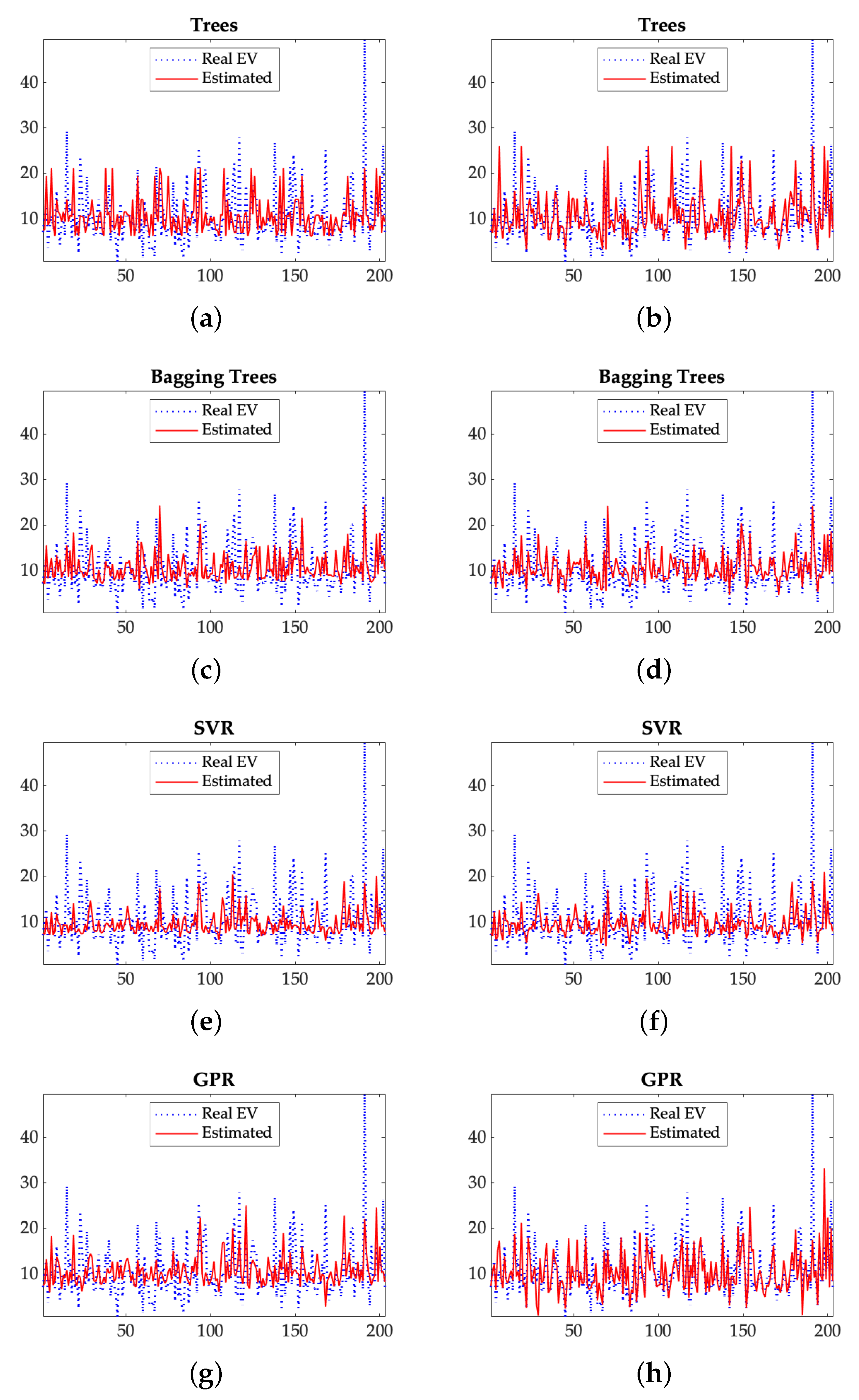
The objective of this subsection was to predict the EV, calculated as the sum of the stock value and the net debt, based on endogenous and exogenous variables examined individually and jointly. Regarding endogenous variables, the projection of FCF for 5 years and the net debt were considered, whereas WACC, GDP, CPI and RIR were evaluated as exogenous variables. Since we explored a range of markets and sectors, operative normalization was applied to each feature, which consisted of dividing the EV by Earnings Before Interest, Taxes, Depreciation, and Amortization (EBITDA) (the gross cash flow that the company can generate). Subsequently, the dataset was split into two new subsets, namely training (70% of samples in the dataset) and test (30% of samples in the dataset). We applied several non-linear supervised ML techniques, such as decision trees, bagging trees, boosting trees, SVR and GPR, all to predict the EV based on endogenous and both endogenous and exogenous variables.

Figure 1 shows the actual normalized EV values (in blue) and their estimated EV (in red) for the described ML methods. The panels on the left ([a], [c], [e] and [g]) show the predictions based on endogenous variables obtained from the DCF method. The panels on the right ([b], [d], [f] and [h]) represent the real and estimated EV when the exogenous variables are also included in the analysis as input data. Visual inspection of charts indicates a tighter relation among estimates and real values when exogenous variables are included in the sample bases. A good example of it is illustrated in panels (g) and (h) corresponding to the GPR technique.

These results are also reflected in

Table 1. Merit figures for the estimated EV models in different scenarios. By rows and grouped according to the companies, we include all the companies or group by sector. In columns, the merit figures for the evaluated scenarios incorporate only endogenous operational normalized variables, and both endogenous operational normalized and exogenous variables. The best method is painted in bold for each performance measure.

		Endogenous				Endo. & Exo.
		MAE	MSE	RMSE	D-Index	MAE	MSE	RMSE	D-Index
All Companies	Linear Regression	4.93	48.89	6.99	0.11	4.49	42.50	6.51	0.11
	Tree	4.33	38.46	6.22	0.10	3.52	26.96	5.19	0.12
	Bagtree	3.85	29.55	5.44	0.12	3.17	19.77	4.45	0.14
	Boosting Tree	5.54	56.13	7.49	0.09	3.91	29.75	5.45	0.12
	SVR	3.84	32.30	5.75	0.10	3.61	28.75	5.42	0.11
	GPR	4.25	34.16	5.85	0.11	2.90	19.70	4.44	0.13
Consumer Cyclical	Linear Regression	3.77	20.82	4.71	0.15	3.30	17.42	4.17	0.14
	Tree	4.23	29.61	5.53	0.12	2.64	11.62	3.42	0.18
	Bagtree	3.00	14.53	3.85	0.17	2.33	9.63	3.12	0.19
	Boosting Tree	3.98	24.33	4.95	0.14	3.34	17.40	4.21	0.16
	SVR	2.73	10.71	3.27	0.20	2.72	11.89	3.45	0.19
	GPR	3.04	15.21	3.92	0.17	1.87	7.82	2.81	0.19
Consumer Non-Cyclical	Linear Regression	6.89	33.30	5.77	0.09	6.14	24.53	4.95	0.10
	Tree	6.08	54.11	7.42	0.10	6.08	54.11	7.42	0.10
	Bagtree	5.63	46.78	6.97	0.10	5.00	34.18	6.13	0.12
	Boosting Tree	5.74	56.94	7.56	0.09	5.03	41.38	6.98	0.09
	SVR	6.24	58.34	7.87	0.09	6.23	54.13	7.83	0.09
	GPR	6.03	55.56	7.58	0.10	4.95	34.97	6.10	0.12
Industrial	Linear Regression	3.56	32.19	5.67	0.13	4.61	24.82	4.98	0.10
	Tree	4.59	50.61	7.28	0.08	5.54	75.86	8.92	0.07
	Bagtree	4.62	43.68	6.65	0.09	3.96	41.07	6.47	0.09
	Boosting Tree	4.62	43.68	6.65	0.09	6.83	114.69	10.91	0.05
	SVR	3.89	52.34	7.24	0.07	3.86	52.20	7.23	0.07
	GPR	4.07	62.25	7.89	0.06	4.78	70.06	8.42	0.06
Technology	Linear Regression	6.94	73.72	8.59	0.09	6.83	71.96	8.48	0.09
	Tree	4.02	27.27	5.28	0.13	3.57	35.31	6.20	0.08
	Bagtree	3.91	18.90	4.99	0.14	3.72	18.03	4.79	0.14
	Boosting Tree	5.83	69.89	8.69	0.07	5.34	59.79	7.87	0.08
	SVR	3.66	31.32	5.60	0.10	3.56	30.42	5.52	0.10
	GPR	4.97	46.32	7.45	0.08	2.41	10.02	3.34	0.18
Utilities	Linear Regression	1.23	1.53	1.24	0.34	1.22	1.38	1.17	0.32
	Tree	1.25	2.10	1.52	0.35	1.24	2.30	1.57	0.34
	Bagtree	1.28	2.60	1.68	0.31	1.36	2.69	1.70	0.32
	Boosting Tree	1.52	3.19	1.89	0.30	1.28	2.35	1.61	0.33
	SVR	1.21	2.17	1.50	0.35	1.21	2.17	1.50	0.35
	GPR	0.97	1.44	1.21	0.40	0.98	1.36	1.22	0.40

and

Table 2. Merit figures for estimated EV models in different scenarios. Rows show the results when grouped by regions or countries, and columns show merit figures for the evaluated scenarios, incorporating either only endogenous operational normalized variables, or both endogenous operational normalized and exogenous variables. The best method is painted in bold for each performance measure.

		Endogenous				Endo. & Exo.
		MAE	MSE	RMSE	D-Index	MAE	MSE	RMSE	D-Index
Brazil	Linear Regression	2.71	8.81	3.16	0.21	2.62	8.54	3.11	0.21
	Tree	2.61	6.79	2.85	0.24	3.23	13.33	3.79	0.18
	Bagtree	2.53	7.60	3.02	0.22	2.23	6.09	2.62	0.24
	Boosting Tree	3.37	12.54	4.09	0.17	3.14	10.37	3.85	0.17
	SVR	1.83	6.14	2.60	0.21	1.85	6.17	2.60	0.22
	GPR	2.01	6.69	2.67	0.22	2.09	7.36	2.74	0.22
India	Linear Regression	5.26	36.27	6.22	0.12	5.46	52.68	7.43	0.09
	Tree	4.73	29.00	5.93	0.12	5.29	35.85	6.40	0.11
	Bagtree	3.85	21.28	4.94	0.14	3.73	20.54	4.83	0.14
	Boosting Tree	5.46	42.99	6.72	0.11	6.38	61.33	8.53	0.08
	SVR	2.70	13.50	3.70	0.16	2.70	13.48	3.70	0.17
	GPR	3.76	24.30	5.24	0.12	3.77	24.46	5.25	0.12
Japan	Linear Regression	3.43	19.29	4.47	0.15	3.50	20.22	4.56	0.14
	Tree	3.14	20.17	4.50	0.13	3.41	38.43	6.41	0.08
	Bagtree	2.35	9.09	3.11	0.19	2.51	9.34	3.37	0.18
	Boosting Tree	4.24	39.77	6.47	0.09	3.98	29.79	5.48	0.12
	SVR	2.16	8.27	2.95	0.20	2.38	12.00	3.47	0.17
	GPR	2.49	14.79	3.89	0.14	2.13	6.27	2.62	0.24
Spain	Linear Regression	3.09	14.55	3.82	0.18	2.05	6.49	2.55	0.24
	Tree	3.11	15.67	3.97	0.16	2.92	13.59	3.69	0.18
	Bagtree	2.35	8.40	2.90	0.22	1.94	6.23	2.50	0.24
	Boosting Tree	2.87	12.10	3.48	0.19	2.61	13.37	3.66	0.16
	SVR	2.45	10.88	3.30	0.18	2.45	10.86	3.30	0.18
	GPR	2.27	9.60	3.10	0.19	1.46	4.04	2.05	0.26
USA	Linear Regression	4.36	37.91	6.20	0.10	4.62	36.44	6.06	0.11
	Tree	4.27	35.94	6.00	0.11	4.42	44.88	6.71	0.09
	Bagtree	3.60	26.84	5.20	0.12	3.50	24.39	4.95	0.13
	Boosting Tree	4.50	34.61	5.88	0.11	4.35	36.40	6.04	0.11
	SVR	3.49	27.03	5.46	0.10	3.51	27.28	5.51	0.10
	GPR	3.73	26.45	5.20	0.12	3.11	19.26	4.39	0.14

, where we also evaluated the impact of the predictions depending on sectors and markets, respectively, considering the RMSE as a key merit of the figure.

Table 1 summarizes the results in terms of MAE, MSE, RMSE and the D-index for all companies, and separately for each industrial sector; consumer cyclical, consumer non-cyclical, industrial, technology and utilities companies. This analysis was developed in two different scenarios: (i) just incorporating endogenous variables, and (ii) taking into account both endogenous and exogenous variables. As a general result, it can be observed that the GPR model showed a certain predominance as the best model when it was considered both internal and external variables. The other way around when only endogenous variables were considered, we could not quite set a best performing configuration. As a general result, we can visualize that prediction error decreased across all methods when exogenous variables were added.

A special interest should arouse the utilities sector, as this sector presented the best ratios in terms of errors (RMSE of 1.21 in best case) and also in contrast with the previous generalized statement, contour information interest should arouse the utilities sector, as this sector presented the best ratios in terms of errors ( did not improve results in any implemented model (RMSE of 1.22 in best case).

Table 2 shows the merit figures for estimated EV models for different regions or countries when either only endogenous operational normalized variables, or both endogenous operational normalized and exogenous variables were incorporated. In general terms, for the different markets, we found that bagging tree and SVR methods, better estimated when only endogenous variables were considered. Moreover, GPR and the SVR methods, can yield better results when both type of variables were included.

3.2. Statistical Analysis of the Best Fitted Methods

We conducted a statistical analysis shuffling randomly over a hundred times, training and test subsets. Results in terms of error were registered as new variables for statistical representation. We considered RMSE as the main figure of merit for this exercise, and the mean and its STD were computed. This type of approach results in a better and more complete representation of estimators’ behavior whether they are presented in consolidated terms, by sector, or by market.

Table 3. Statistical analysis of one-hundred realizations of the best performing models, for different input-space subset scenarios. In rows, industries and region subsets. In columns, mean ($\mu$) and STD ($\sigma$) of RMSE, for the scenarios including (i) endogenous variables, and (ii) both endogenous and exogenous variables.

		Endogenous		Endo.&Exo.
		$\mathit{\mu }$	$\mathit{\sigma }$	$\mathit{\mu }$	$\mathit{\sigma }$
All Companies	Bagtree	5.74	0.52	4.75	0.53
	SVR	6.21	0.58	5.43	0.53
	GPR	6.16	0.48	4.88	0.64
Consumer Ciclical	Bagtree	3.93	0.46	3.46	0.49
	SVR	3.91	0.47	3.62	0.45
	GPR	3.97	0.48	3.32	0.45
Consumer Non-Ciclical	Bagtree	5.88	0.74	5.38	0.56
	SVR	6.35	0.74	6.15	0.74
	GPR	6.16	0.80	5.51	0.49
Industrial	Bagtree	5.23	2.03	5.72	2.30
	SVR	5.64	2.11	6.01	2.37
	GPR	6.55	2.32	6.79	2.06
Technology	Bagtree	9.17	3.68	8.00	3.22
	SVR	9.19	3.61	8.09	3.26
	GPR	9.80	3.84	6.95	3.92
Utilities	Bagtree	1.54	0.35	1.56	0.37
	SVR	1.34	0.29	1.37	0.33
	GPR	1.39	0.41	1.44	0.44
Brazil	Bagtree	3.16	0.45	2.94	0.45
	SVR	3.03	0.50	3.03	0.50
	GPR	3.14	0.54	3.09	0.60
India	Bagtree	7.11	2.04	6.66	1.87
	SVR	6.76	2.02	6.84	1.88
	GPR	7.14	1.97	7.64	1.71
Japan	Bagtree	6.72	3.43	6.70	3.54
	SVR	6.57	3.01	6.42	3.11
	GPR	8.22	3.29	4.80	2.91
Spain	Bagtree	3.17	0.43	2.76	0.40
	SVR	3.22	0.50	3.34	0.52
	GPR	3.27	0.50	2.21	0.39
USA	Bagtree	5.36	0.56	4.51	0.52
	SVR	5.47	0.71	5.40	0.60
	GPR	5.25	0.54	3.95	0.53

depicts these results when the previously outperforming ML techniques were applied, specifically bagging trees, the GPR, and the SVR. The comparative analysis between the exclusive generalization capabilities of endogenous variables, versus the evaluation of both endogenous and exogenous characteristics, consolidated previous results of the incremental predictive power of exogenous information in terms of the mean. In terms of STD no significant difference was found among this two scenarios.

Uneven performance was observed in the analysis of the models when they were consolidated by sectors of activity in different markets. In the case of consumer activities, both cyclical and non-cyclical highlighted that the incorporation of exogenous information does not add predictive power to the ability to approximate the company’s valuation. Note the low STD of the errors and their high mean obtained for these sectors. The mean was especially high for non-cyclical activities.

For the industrial sector, it was observed that the valuation capacity of the models worsened when exogenous variables were incorporated. The high STD observed, which was up to four times higher than in the case of consumer companies, stood out. The technology sector showed singular behavior, as there was noticeable worsening of the averaged errors produced in the valuation model when external information was incorporated into the company. However, the high variability of the model was significantly reduced when exogenous variables were also considered. For the utilities sector, the analysis reflected stable behavior without apparent variation when exogenous information was incorporated. For this sector, results were outstanding in terms of the mean and the STD.

The analysis of the results obtained for the different markets showed visible differences in behavior when grouped in emerging and consolidated markets. In particular, independence was noticeable in emerging markets when the presence of exogenous features was considered. The slight improvement in both the mean and the STD of the prediction error when exogenous variables were included, outlined the noticeable independence in of this market from contour variables. However, different results were found in consolidated markets. The analysis of over 30 years historical data for countries such as Japan, Spain and the USA (addressed jointly hereafter as the consolidated markets) showed that the incorporation of exogenous variables improved the predictive capability, as it was found reduced in terms of the mean and to some extent in the prediction variance. Nevertheless, noting the unequal accomplishment of the models for these two market groups, the bagtree performed better for emerging markets (Brazil, and India), whereas the winning method for consolidated region was GPR.

3.3. Feature Evaluation Capabilities

Although any variable could be considered to be additional information, and to some extent could add value to a sample base, large number of different variables could also create difficulties to ML convergence. In one side, the number of variables should always remain in several orders of magnitude lower than the number of samples. Second, the excess of information, duplicated, or just uncorrelated with the final goal, could limit the convergence capabilities, lead to local minimums, lead to overfitting, and/or increase the computational cost. Therefore, it is often appropriate, and even necessary, to follow a certain strategy to make sure that we are considering the right and most relevant features from our datasets. Therefore, one key goal in ML implementation is to select the key features to improve the precision performance and to provide fast and effective tools, which at the very same time offers a sensitive scenario. For additional information and better understanding see [41].

Although several the statistical learning methods presented in this work exhibited to be robust against the incorporation of variables, as the SVR, it is not always easy to establish an automatic or implicit procedure for select the features that can drive better results. Hence, in this study, a good number of experiments were carried out with different configurations that characterize and evaluate the features in the input space for the proper fine-tuning of the models. As mentioned earlier, in this study we have considered the operational normalization of the input variables as the base scenario for the analysis. However, to verify the results in other possible input space, we also reproduced the analysis simultaneously by applying the operational and statistical normalization as defined in the companion paper.

Table 4. Result comparison based on RMSE for better performing ML implemented techniques. Columns from left to right: (i) endogenous variables with operational normalization; (ii) endogenous and exogenous variables with operational normalization; (iii) endogenous variables with operational and statistical normalization; (iv) endogenous and exogenous variables with operational and statistical normalization; (v) extended features, incorporating additionally to previously defined endogenous and exogenous, the NPVs developed in previous paper; and (vi) the most relevant features in double-normalized endogenous and exogenous variables, namely: first year FCF, net debt, RIR and GDP.

	Oper. Nor.		Oper. & Stat. Nor.		Extended	Key
	End.	End. & Exo	End.	End. & Exo	Features	Features
Linear Regression	6.47	6.02	6.47	6.02	6.16	6.12
Tree	6.22	5.19	6.54	5.63	5.50	5.32
Bagtree	5.44	4.45	5.33	4.50	4.63	4.75
Boosting Tree	7.49	5.45	7.49	5.46	5.81	7.20
SVR	5.75	5.42	6.00	5.37	6.29	5.39
GPR	5.85	4.44	5.85	4.44	4.57	5.01

shows the results obtained when only endogenous variables were considered, and with endogenous and exogenous variables jointly incorporated. A comparison of scenarios revealed that the findings were consistent with those expressed earlier. A slight improvement was found when exogenous variables were included, but no significant differences were identified after statistical normalization.

An equivalent analysis was carried out to assess the incremental valuation aptitudes of the complex estimated variables that are usually incorporated in valuations by analysts, in particular the NPVs defined and calculated previously described in the companion paper. The results indicate that the incorporation of these compounded estimates, subordinated to the main ones already present in the input space, did not add predictive capacity to the model, as showed in Table 4 (Extended Features column).

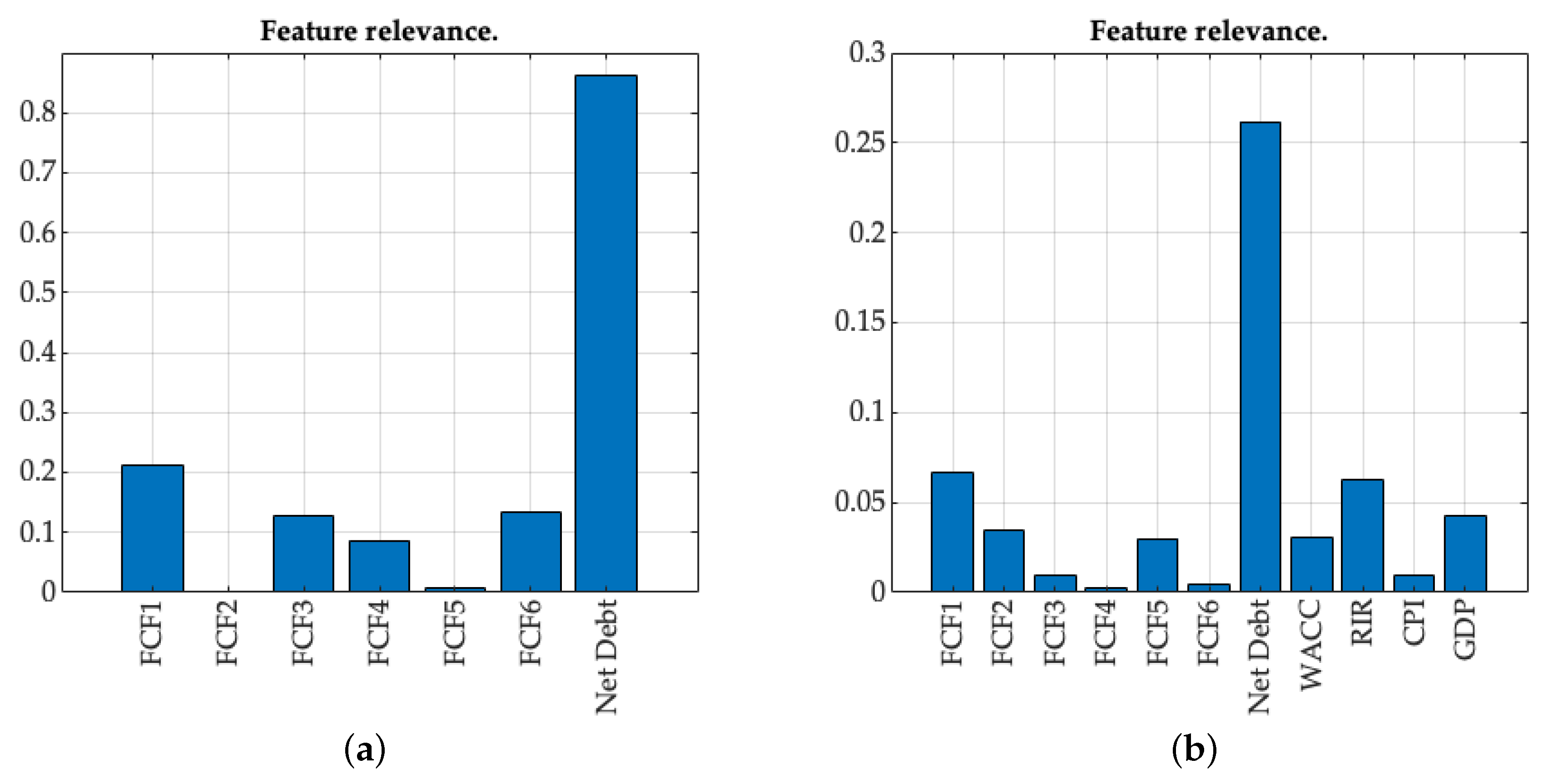
Once confirmed that neither the incorporation of double normalization nor the addition of complex, generally accepted, subordinated variables incremented the classification or regression capabilities of the implemented methods, we evaluated subsets of variables. The aim was to define a computationally low-complexity model by choosing the features that consistently showed greater relevance when decision trees were evaluated, although not in all realization and methods in the same order: first year FCF, net debt, GDP and RIR. An illustrative example of this relevance is presented in Figure 2 for only endogenous (a), and for both endogenous and exogenous (b) variables. The results of this simulation, presented in the last column of Table 4 (Key Features column), showed that the exclusive use of the four most significant variables either slightly worsened or matched the results obtained in the base case scenario considering endogenous and exogenous operationally normalized variables.

3.4. Trend Analysis

As mentioned in the preceding sections, the DCF method is undoubtedly the most commonly used method when the potential value of a company is analyzed. It was also explained that the main drawback of this method is that it is highly sensitive to certain precise parameters. In order to estimate this dependence, and to validate the model when the valuation ranges around any targets value, a sensitivity analysis is commonly incorporated as part of the equity valuation study [4,15]. However, this type of analysis or technique allows the underlying business model to be validated, especially when the complex interrelationships among the variables in the model, make it necessary to confirm that the expected trend is consistent around a valuation set point. To this end, we created a trend analysis to appraise the consistency of the addressed models.

The model must be valid over a wide range of input values, and there is the additional complexity of establishing the evenness point or simultaneous valuation set point for all companies, regions and sectors. Consequently, double normalization (operational and statistical) of the input variables had to be applied. Once both normalizations had been applied, all variables in the input space presented null mean and unit variance, and the trend analysis could then be carried out in the range of one time the STD, in another words, input variables ranging from −0.5 to 0.5.

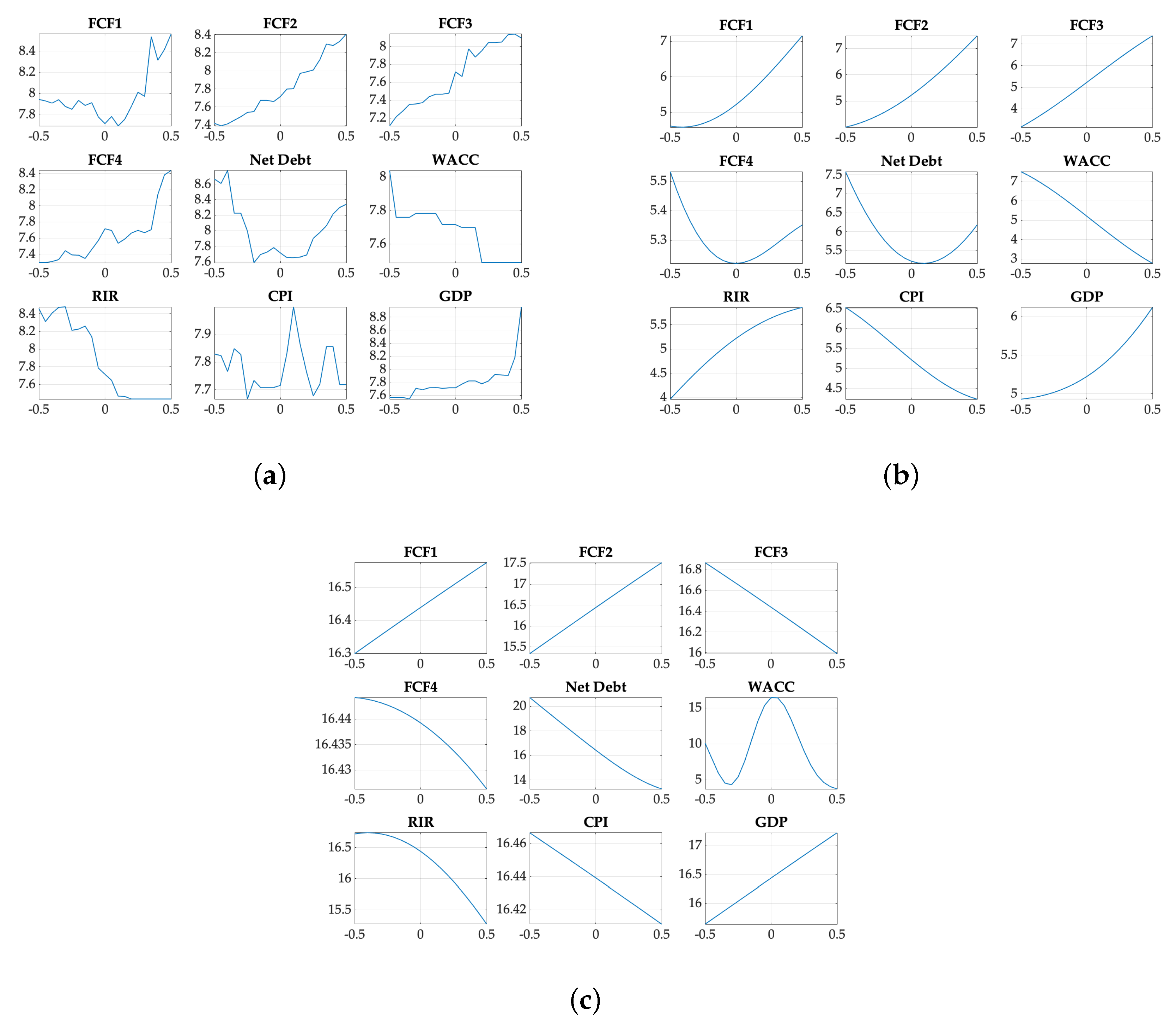
Figure 3 shows the local trend of widely understood key variables, for a better performing method (BagTree, SVR and GPR). The abscissa axis corresponds with the double-normalized variables, and the ordinate axis represents the operationally normalized output, EV/EBITDA. Visual inspection of these charts are recurrently coherent with expected trends, as the output showed a positive response versus the different FCF, CPI and GDP, whereas this response was inverse versus net debt, WACC and RIR. Individual exceptions were found in certain realizations and for a limited number of variables. In that direction and from illustrative proposes, the outcomes depicted in these figures, acknowledged this reality for variable RIR in Figure 3b and FCF3 and WACC in Figure 3c.

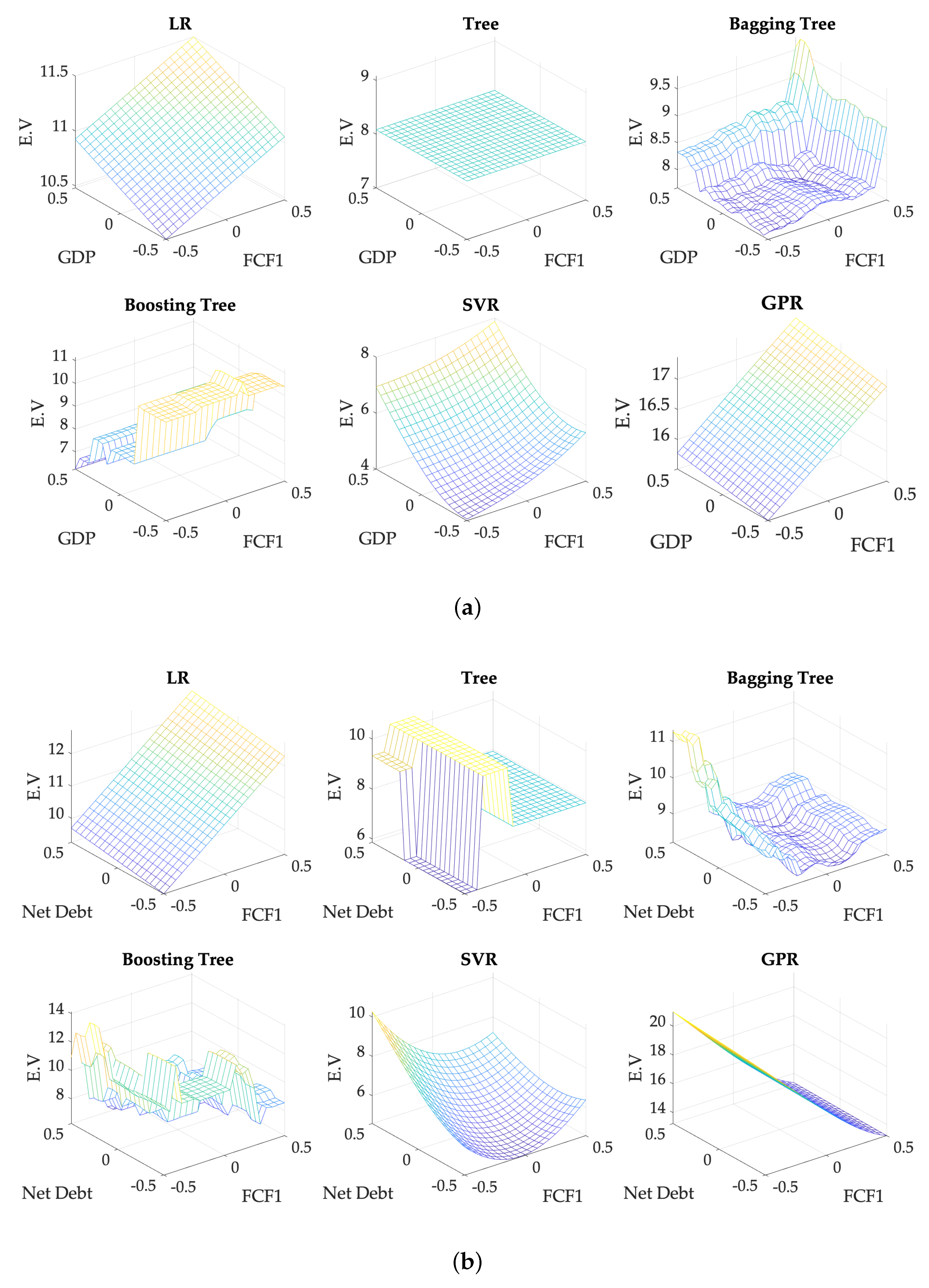
Same rational, but this time in a bi-variant input space, is showed in Figure 4. Homogeneously to the one-dimensional approximation, visual inspection of the surfaces, showed a broad coherence with expectation in the two-dimensional local trend. But again individual exemptions were found and analyzed arising equivalent findings as in the one-dimensional representation.

4. Discussion and Conclusions

In the companion paper we evaluated different techniques to develop an unbiased valuation model, leveraging especially on accounting information and on the widely accepted DCF method. In this second work, we pursued the very same objective, but throught an intensively ML approximation, and evaluating the performance capabilities up to 18 different learning algorithms using the following set of techniques: LR Algorithms, Regression Trees, Ensembles of Trees, SVR, and GPR.

As a main conclusion of this work, we could state that it is possible to create an unbiased valuation model that narrows the more than relevant uncertainty by strictly following market expectation, based on state of the art ML techniques. These algorithms could eventually support, contribute, or validate valuation ranges that are especially useful in corporate developments and risk assessment. The methods and variables incorporated in different analysis showed an uneven generalization capacity, attending to markets region and industry sectors, and thus suggesting the use of specialized learning processes for specific purposes. SVR, BagTree, and GPR were identified as the methods providing the top performance over the different implemented scenarios. None of these three was identified as a universal top performer for all evaluated scenarios, although SVR can be said to remain as the one that most regularly followed the top performing method.

Under a full consolidated valuation perspective, ML techniques exhibited a limited ability to generalize for blind valuation when historical intrinsic accounting information was exclusively implied. Moreover, the incorporation of exogenous information offered just a slender improvement in the estimation capability for this global consolidated approach.

As far as business activities are concerned, we can argue that SVR, BagTree, and GPR closely followed market expectation for the utilities sector, and up to a certain extent for consumer products, cyclical and non-cyclical. And even more, in both cases, the valuation capacity of the models was invariant against macroeconomic differences, showing high stability across markets. In this case, RMSE reached the minimum uncertainty with an average error lower than 1.5 times EBITDA, and also the lowest entropy, revealed in STD values not higher than 0.4. Therefore, it can be said that the availability of sector relative and qualified information contributes significantly to ML models in utilities and consumer products across regions, which is especially true for utilities.

In the opposite side we found the industrial and technological sectors, which yielded much higher statistical errors, both in terms of the mean and the STD. Therefore, we can say that these two sectors, from a business perspective might be considerably bundled to other realities not represented in a cross-region industry view. We can argue also that local markets dynamics, country specifics economic, and their much more complex underlying business model, make non-viable the concept of a general consolidated industry-focus scenario.

Limited prediction accuracy and unparalleled results are shown when the analysis is performed by market regions, particularly if we split them attending to maturity into emerging and consolidated. A meager dependence was found when exogenous variables were included in emerging markets, and the other way around, this relationship was more intense in consolidated markets. Along with the difference in results and behavior of the valuation models in this regional setup, and for these two separated space-sets, it might be suggested to elaborate more on expanding even further the methods and algorithms, and to consider different sampling structure of the analysis combining markets and sectors for a deeper and closer correlation among peers. For this reason, we consider as a promising next step to implement a much larger effort in the number of companies incorporated in the study, so that a simultaneous double split, by sector and by market, approach, could allow a sufficient sample base for the statistical significance in double-classified companies.

Trend analysis was in general coherent, although singular cases were found when globally consolidated. This was consistent with previous findings, suggesting that the lack of structure in the data in a global approach could be causing convergence difficulties in experimental setting, such as overfitting or local minimum model lock-up.

With these results and taking into account the aforementioned conclusions, we can finally argue that the stability of the consumer segments allows a closer assessment related to the accounting reality of each company throughout the markets. This is especially true in utilities and to lesser extent in consumer products, whether cyclical or non-cyclical. On the other hand, and due to the more complex reality of business, a closer description of the estimates of industrial and technology sectors may require either more sophisticated methods, additional information, further structuring models, or a much wider dataset. In general terms, we could also highlight that although the presence of exogenous variables improved the results, this improvement was not always enough to positively compare against utilities. It goes without saying that regardless of the potential improvement that could be achieved with a double segmentation of the sample space, it does not detract any value to the relevant findings of this work. The results provided sufficient statistical significance, and therefore, paved the way for the creation of unbiased method to assess valuation ranges considering simultaneously several operational variables from the company itself and its peers.

As a global conclusion, we would like to modestly assess that the methods presented here, especially Decision Trees, SVR, and GPR, could support relevant complementary and alternative priceless information guidance, for valuation and risk assessment, especially in private equity. This modeling capacity is equally sufficient, regardless the availability of other complexes subordinate variables, such as FCFs forecast or NPVs. All this leads us to further argue on how these techniques could move ahead the traditional complex forecasting techniques, when industry and general economic information is available.