On the Differential Analysis of Enterprise Valuation Methods as a Guideline for Unlisted Companies Assessment (I): Empowering Discounted Cash Flow Valuation

Abstract

The Discounted Cash Flow (DCF) method is probably the most extended approach used in company valuation, its main drawbacks being probably the known extreme sensitivity to key variables such as Weighted Average Cost of Capital (WACC) and Free Cash Flow (FCF) estimations not unquestionably obtained. In this paper we propose an unbiased and systematic DCF method which allows us to value private equity by leveraging on stock markets evidences, based on a twofold approach: First, the use of the inverse method assesses the existence of a coherent WACC that positively compares with market observations; second, different FCF forecasting methods are benchmarked and shown to correspond with actual valuations. We use financial historical data including 42 companies in five sectors, extracted from Eikon-Reuters. Our results show that WACC and FCF forecasting are not coherent with market expectations along time, with sectors, or with market regions, when only historical and endogenous variables are taken into account. The best estimates are found when exogenous variables, operational normalization of input space, and data-driven linear techniques are considered (Root Mean Square Error of 6.51). Our method suggests that FCFs and their positive alignment with Market Capitalization and the subordinate enterprise value are the most influencing variables. The fine-tuning of the methods presented here, along with an exhaustive analysis using nonlinear machine-learning techniques, are developed and discussed in the companion paper.

1. Introduction

Estimating the fair price of a company or the Enterprise Value (EV) is a major issue in academic and business literature, as it has relevant impact in a number of situations. Global corporate operations, mergers and acquisitions, alliances and joint ventures, corporate bond issuing, international public offerings (commonly IPOs), banking credit, portfolio management, risk assessment, and in some cases the top-management bonus, require fair valuations compelling with well-founded and generally accepted systematic assessments [1,2,3,4,5,6,7]. Investors, analysts, and sometimes academics tend to approach this objective focusing in public companies, for which a large amount of information and knowledge is available. However, this working line conveys the development of tight tailored models, with relevant chances to overfit the selected target, and subsequently lacking generalization capability over time, sector, market, or region. In this category we can include the investment banks’ Investor Research (IR) reports and the Technical Analysis (TA) reports [8,9,10,11,12,13,14,15].

Starting with this second group, TA reports support their models on market behavior and heuristic estimates, solely funded on historical price-volume data. In this case, forecasting estimates rely on trading rules attached to chart patterns fully dissociated from fundamental business data. Alternatively, investment banks and consultancy firms base their IR reports on deep industry knowledge and on available business information. This way of proceeding is generally known as Fundamental Analysis (FA), as it uses historical and solid financial statements (fundamentals), as well as commercial business forecasts [1,7,16,17,18]. This methodology offers a much more rigorous and deeper understanding of the company real activity, although such a deep knowledge may limit the generalization capabilities.

Additionally to these very well established and known approaches, academics have also proposed statistical and mathematical methods with the aim of dissociating the tailoring and tight-fitting approach of IR and FA reports. This particular setting is especially noticeable in recent studies where machine learning techniques are applied to credit risk assessment and stock pricing forecast [19,20,21,22]. Under this view, in an attempt to categorize these methods, and attending to the nature of the supporting variables, we propose to classify them into three basic categories, namely, balance-sheet statements, Income Statements (also known as multiples), and value-creation approaches [23], as shown in

Table 1. Compilation of company valuation methods based on financial statements.

Balance Sheet	Income Statment	Cash Flow Statment
		DCF	Value Creation	Options
Book Value	PER	Free Cash Flow	EVA	Black and Scholes
Adjusted Book Value	Sales	Equity Cash Flow	Economic Profit	Investment Options
Liquidation Value	P/EBITDA	Capital Cash Flow	Cash Valued Added	Expand the project
Substantial Value	BAIT	APV	CFROI.	Delay the Investment

.

The first set of methods, or balance-sheet based methods, are based on pre-existing accounting information in company records and they are strongly supported by balance-sheet statements and book value related ratios [24]. These methods usually define and apply specific corrections to actual statements by incorporating contextual factors, such as future taxes, good-will, unrealized capital gains, or project finance associated variables. A remarkable reference, and probably the most cited academic work in this area, is the Adjusted Book Value proposed by Graham in its different editions [14,25]. The second set of methods are the multiples based methods, also known as comparable methods, which use the effective value of other operations as a benchmark to extrapolate to current valuations. Examples of references for benchmarking purposes are stock price, comparable corporate operations, balance-sheet ratios, and consensus investor-related valuation reports. IR reports always incorporate this information as a back reference for validation and support for the valuations stated in the reporting document [7,26,27].

The third set, or value-creation based methods, includes the Discounted Cash Flow (DCF) as the most remarkable and frequently used tool for large-company valuation [16,28,29,30,31,32]. Another method also included in this set is the now popular Residual Income Model (RIM) [33,34,35,36]. Both DCF and RIM are based on the discount to date of future economic flows, and specifically the Free Cash Flow (FCF) for the DCF method, and the net future residual income plus the capital of the firm in the case of RIM method [4]. The DCF method is essentially the actual discount of future FCF, which stands for the company cash flows that are real and effectively free and available to be applied in favor of shareholders. The nature of this model is independent from the effective payback strategy that the company finally executes, understanding that it would always be the most adequate and profitable one for equity holders.

The discount rate to be applied to FCF, and generally referred as Weighted Average Cost of Capital (WACC) [29] requires especial remark at this point. This rate, in its closed form, includes two particular sensitive parameters, namely the risk-free rate (or the expected returns of an asset that is considered risk-free) and the risk premium of the company (or the differential among expected return of the specific commodity and the risk-free asset), also called beta ($\beta$) [37]. Academics generally agree on the WACC closed form, although there is not a consensus on how to evaluate or estimate the mentioned specific components [30,31]. This fact has led to a wide extend of unrelated application of value creation models. Meanwhile the RIM model is also centered on the creation of value to shareholder, but in this case it is defined as the effective accounting earnings of the year. Accounting earnings are discounted to date using the cost of equity ($Ke$), which is one of the components of WACC. The RIM model very much compares with DCF model, since it is based on the same idea, but it focuses on shareholders value creation, so that it is directly linked to market value. One important drawback of value creation methods is the requirement of information such as forward statements, forecast, or detailed information effectively only available for large and public companies, but rarely for private entities.

In addition to the previously mentioned methods, statistical learning and Machine Learning (ML) techniques have received increasing attention in the financial field over the years [38]. Examples of these applications are the prediction of bankruptcy [39,40], debt and credit rating classification, or follow-up analysis and pattern detection in stock-quote series [41,42]. However, and to the best of our knowledge, no prior analysis have been effectively implemented using these techniques in the company-valuation field [43,44]. This might be due to the relevant complexity and the large number of variables involved. Hence, we can argue that there is still room for development in terms of how statistical learning algorithms could eventually contribute to this end, as it has been the case in other relevant disciplines [45,46].

All things considered, the main goal of this work is to analyze and propose an unbiased quantitative systematic company-valuation model [1,4,27,30,35,47,48], which should be able to approximate company value based on current financial information, historical accounting records, global economy framework information, as well as market trend by sector and region. To do so, and bearing in mind that the value-creation approach (and more precisely DCF) is probably the most described and applied model, we proposed to analyze this method applying a number of different strategies for standard FCF forecasting and WACC computation, while leveraging strictly on reported historical financial statements extracted from Thomson Reuters Database. For this study we took into account the full balance sheet and profit-and-loss statements in 30 consecutive years for a representative set of 42 companies, from five industrial sectors and within five market regions. In an additional final analysis included in this paper, we presented our first step into a more complex mathematical implementation, as an starting point toward more sophisticated methods, by incorporating exogenous variables together with the previously obtain features in order to build and asses the incremental generalization capabilities of linear regression techniques.

In the companion paper [49], and once having developed and compared in this current work different company-valuation strategies and their ability to generalize the intrinsic value of companies, we present a deep and thoughtful comparative of ML techniques in this setting. In particular, we extend therein the analysis to nonlinear regression techniques using the variables that in this work were proven to be more closely related to the actual EV. Furthermore, we include a set of endogenous and exogenous variables with documented influence on the valuation according to the literature [50].

This paper is organized as follows. In Section 2, we describe the tools and databases, the DCF implemented methodology, and the Linear Regression Techniques used in this work. In Section 3, we present several relevant experimental results, namely, FCF forecasting benchmarking, WACC inverse method analysis, DCF valuation results, and linear regression analysis. In Section 4, we present the discussion and the main conclusions.

2. Methods and Materials

2.1. Database and Tools

For the purpose of this work, we took into consideration information from heterogeneous market regions for their benchmarking, consisting of Spain, United States, Japan, Brazil, and India. We analyzed five sectors, namely, consumer cyclicals, consumer non-cyclicals, industrials, technology, and utilities. A total of 42 companies were considered and classified according to their sector and market region, as shown in

Table 2. Companies analyzed according to market regions and sectors.

	Sector	Consumer Cyclicals	Consumer Non-Cyclicals	Idustrials	Technology	Utilities
Market
Spain		Inditex	Baron de Ley	Ferrovial	Telefónica	Endesa
		Melia	DIA	ACS	Amadeus	–
United States		Starbucks	Wal-Mart	FedEx	–	AEP
		–	Coca-Cola	3MCo.	Microsoft	Edison
Japan		Toyota	Asahi	Kajima	Sony	Chubu EP
		Honda	Shiseido	Shimizu	Rakuten	TEPCO
Brazil		Grendene	AmBev	Azevedo	Tim	CEMIG
		Alpargatas	–	MRV	–	CPFL Ene.
India		Maruti	Dabur	Reliance Infr.	Tata Commu.	–
		Mahindra	ITC	–	Bharti Airtel	–

. The available financial information depended on each company, varying from 5 to 30 years.

We used the intrinsic information (endogenous variables) obtained from the financial statements, namely, balance-sheet, income statement, capitalization, and several financial ratios available in Eikon Thomson Reuters Database. This database consolidates the financial information obtained from the reports published by the companies, rigorously verified and monitored by nearly 45,000 professionals of the firm worldwide. It is considered one of two largest and most important financial information databases in the world, covering 99% of listed companies in 170 countries and 60 sectors [51].

Furthermore, we evaluated exogenous variables, including the following ones: Consumer Prices Index (CPI), which measures changes in the price level of market basket; Real Interest Rate (RIR), which shows the difference between nominal rates and inflation, and it is a good driver for companies financing cost; Gross Domestic Product (GDP), which is included because it features general gross growth of a country and it consolidates the growth capability in markets, and so do companies to a greater or lesser extent [52]. For mathematical, statistical, and data modeling, we used MATLAB [53]. This flexible software tool allowed us to design, analyze, and evaluate the proposed scenarios and simulations, and also to set the structure to extend results from single company valuation experiments to a larger scale, which was especially relevant when ML techniques were to be subsequently proposed and applied.

2.2. The Discounted Cash Flow Method

As previously mentioned, the DCF model is one of the most trusted methods for valuating companies because of its ability to generate equity for the shareholder [1,16,30,54,55]. This model computes the EV based on the FCF forecasts. FCF is the amount of money available to cover the debt or to pay back equity holders, and it can be considered as a measure of the financial capacity of a company. It is obtained as follows,

$$FCF=NI+A+DEP-CapEx-\Delta WC$$

(1)

where NI is the Net Income, A is the Amortization, and DEP is the Depreciation. All of them are recorded at the income statement. The Capital Expenditures is given by $CapEx=PP{E}_n-PP{E}_{n-1}+A+DEP$, where PPE is the Property, Plant, and Equipment of a company, recorded at its balance-sheet, and n represents any specific year. The Working Capital (WC) is determined by $WC=CA-CL$, being these values recorded at the balance-sheet as Current Assets and Current Liabilities, respectively. Finally, $\Delta WC$ stands for the change of $WC$ in consecutive years. The FCF forecasts, represented in this work as $FC{F}_{n+1}$, are usually calculated for 5 to 10 years at a growth rate (r) [1,56,57].

The first three calculations are based on the year-by-year growth for consecutive $FCF\left(r_{FC{F}_n}\right)$, being this ratio complying with $FC{F}_n=FC{F}_{n-1}(1+r_{FC{F}_n})$. For these three models, r is calculated as the mean, median, and Compound Annual Growth Rate (CAGR), of the last 5 years (see

Table 3. FCF forecast strategies.

Linear Constant	$FC{F}_{(n+1)}=FC{F}_n\times (1+{mean}_{i=n-4}^n\left(r_i\right)$)
Median	$FC{F}_{(n+1)}=FC{F}_n\times (1+{median}_{i=n-4}^n\left(r_i\right))$
CAGR	$FC{F}_{(n+1)}={FCF}_n\times (1+CAGR)$
Polynomial of 2	$FC{F}_{(n+1)}=p_0+p_1\mathbf{x}+p_2{\mathbf{x}}^2$
Polynomial of 3	$FC{F}_{(n+1)}=p_0+p_1\mathbf{x}+p_2{\mathbf{x}}^2+p_3{\mathbf{x}}^3$

). The CAGR is given by

$$CAGR={\left(\frac{FC{F}_{n-1}}{FC{F}_{n-k}}\right)}^{1/(n-k)}-1$$

(2)

where k is the number of consecutive years included in the analysis, for the CAGR calculated to be applied to years n and onward. Finally, we compute the FCF forecast based on the coefficients $\left(p_i\right)$ of polynomials of degree 2 or 3 (see Table 3 for details), which are obtained from the previous five FCFs. Vector $\mathbf{x}=[n-1,n-2,n-3,n-4,n-5]$ represents the years.

The DCF method uses the discount rate WACC for measuring the cost-opportunity of companies to use their own equity (E) and debt (D) to finance their activity and generate a cost of capital [24]. The WACC is formulated as follows:

$$WACC=K_e\frac{E}{D+E}+K_d\frac{D}{D+E}$$

(3)

and it has the following components. First, the cost of equity ($K_e$) is the minimum return required by equity holders and it is given by the expression $Rf+\beta (Rm-Rf)$, where the risk-free rate (Rf) is generally assimilated to state bonds, $\beta$ indicates the inherent risk factor of the company in relation to the market, and $Rm$ is the average profitability of the market where the company is stabilized. Second, the cost of debt holders ($K_d$) is given by $int(1-T_m)$, where $int$ represents the effective interest rate that the company is paying to support its debt and $T_m$ represents the effective company tax-rate. Third, the percentage that the equity takes in company financing terms is $\left(\frac{E}{D+E}\right)$. Finally, the equivalent rate from the proportional debt is $\left(\frac{D}{D+E}\right)$, considering also the applied effective tax-rate. Taking into account that in theoretical terms companies are created to last forever, future business and value need to be represented. This term is usually consolidated as the sum of the infinite geometric series of FCFs, discounted with the mentioned WACC and growth. The closed expression for the Terminal Value ($V_n$), or expected returns discounted to date of all future FCFs till perpetuity, is given by

$$V_n=\frac{FC{F}_{n-1}(1+g)}{(WACC-g)}$$

(4)

where g represents the growth rate to perpetuity for the FCFs, $FC{F}_n$ represents the last forecasted $FCF$ of the model, and the WACC corresponds almost in all cases with the short term estimated WACC, although this might vary among authors [1,57]. The estimation g is capped by the expected long term world growth rate, and it can be estimated by the Gordon growth model [54], which assumes the g is within historical rates of inflation. Therefore, we can compute the Net Present Value (NPV) as follows:

$$NPV=\frac{FC{F}_1}{(1+WACC)}+\frac{FC{F}_2}{{(1+WACC)}^2}+\cdots +\frac{FC{F}_{n-1}}{{(1+WACC)}^{n-1}}+\frac{V_n}{{(1+WACC)}^n}$$

(5)

2.3. Adjusting DCF: The Forecasting Strategy

DCF model is extremely sensitive to certain components of Equation (5), specifically the FCF forecasting strategy, and the figure applied as discount rate, the WACC [1,58]. In this subsection we pay attention to the strategy established, both to set the forecasting baseline as well as to set the growth rate to be applied for future FCFs. It is precisely at this point where investment analysts offer complete and extensive justifications for the proposed models inside Equity Research Reports. As previously mentioned, the objective of this work is to develop an unbiased mathematical model that does not require additional interpretable information which: (i) might not be available; (ii) requires relevant interpretation; or (iii) a qualification or quantification is needed to be implemented. For this reason, this study proposes several forecasting methods based exclusively on the financial information available in accounting reports from companies. In this work a number of strategies have been developed to establish the baseline based on the figures from previous years, and projections, but not too exhaustive effort was devoted to this end. Authors also scrutinized much more sophisticated baseline assessment models and projections in the pre-programming phase, namely a number of regression models, but they were not finally implemented due to two reasons. Firstly, since they had not been justified by literature, the exercises carried out for individual companies did not outperformed the lesser complex ones, and instead the relevant increment in complexity suggested not doing so. Secondly, the authors assumed that such complexity and effort could be much more effective when machine learning algorithms were applied to the final valuation (see the companion paper).

In this work, we propose and analyze five different FCF forecasting strategies, namely, Linear Constant, Median, CAGR, and Degree-2 and -3 polynomial fitting, as shown in Table 3.

2.4. The Inverse Method

Continuing with previously described rationale, the second key element that plays a huge and meaningful impact on the final valuation is the WACC. In this direction, although a relevant number of authors agree in the closed equation described in detail in previous sections, it is not such a consensus in the way its constituents are or could be calculated, leading to a significant uncertainty in final results.

In an attempt to evaluate WACC, in this paper we propose a backward perspective to obtain the discount rate value. In consequence, this approach computes the implicit valuation of the stock market for each forecasting predefined method. In this analysis we gauge a single and effective WACC for each company, year, and DCF model, which is later consolidated across companies, years, markets, and regions. Aside from these jointly combined values that could eventually be extended to private equity valuation, the presented results provide a qualifying attempt to evaluate, compare, and validate the different forecasting strategies presented in this paper by using the appropriate statistical measurements.

2.5. Linear Regression Technique

Statistical learning techniques have the ability to learn from samples [59,60,61]. In this work, an initial analysis is performed using the well-known technique called linear regression, which is a parametric method used to describe a continuous response variable (y) as a linear function (f) of one or more variables ($x_l$). We denote $\left\{{({\mathbf{x}}_i,y_i)}_{i=1}^m\right\}$ as the data set, where m represent the number of samples. The linear regression model is defined as follows:

$$\widehat{y_i}={\mathbf{w}}^{⊺}{\mathbf{x}}_i+{\epsilon }_i$$

(6)

where $\widehat{y_i}$ is the estimated response, $\mathbf{w}={[w_0,w_1,\dots ,w_l]}^{⊺}$ are the coefficients of the linear model, with l the number of variables, and ${ϵ}_i$ is the error or perturbation for the i-th observation. In order to find linear model coefficients w, a least-squares strategy is usually used, which consists of minimizing the square objective function:

$$\widehat{\mathbf{w}}=\underset{\mathbf{w}}{argmin}\left|\right|\mathbf{y}-\widehat{\mathbf{y}}{\left|\right|}_2^2$$

(7)

where $\mathbf{y}={[y_0,y_1,\dots ,y_m]}^{⊺}$. In order to evaluate the performance of the linear regression model, we compute different figures of merit, namely, Mean Absolute Error (MAE), Mean Squared Error (MSE), and Root Mean Square Error (RMSE), which are calculated as follows,

$$MAE=\frac{1}{m}\sum _{i=1}^m|{\widehat{y}}_i-y_i|$$

(8)

$$MSE=\frac{1}{m}\sum _{i=1}^m{({\widehat{y}}_i-y_i)}^2$$

(9)

$$RMSE=\sqrt{\frac{1}{m}\sum _{i=1}^m{({\widehat{y}}_i-y_i)}^2}$$

(10)

3. Results

This section includes the results of the experiments performed in this work to either validate or reject the hypothesis that it is possible to conduct an unbiased company valuation without being subject to qualitative aspects which are hardly quantifiable. Toward that end, we used stock market EV as the target, using exclusively the information that was available for both listed and unlisted companies, and supported on the mostly accepted ones by investors and analysts thoroughgoing developed DCF valuation model. To do so, and with the aim of evaluating the behavior of key variables of DCF model, we first scrutinized the existence of applying an effective WACC for each sector, market, and region that fit the model by matching the EV through different systematic cash flow forecasting methods. Specifically, the proposed implementation approach exercised the inverse method to estimate the WACC that better approximated current EV, considering a number of different FCF forecasting strategies that are described in Table 1. In a second approach we applied the direct method based on the reference WACC values reported in literature to better assess again the right EV over the mentioned forecasting strategies. Finally, we started to explore the potential of the ML techniques, limiting ourselves here to the linear regression capabilities for the very same aim, and not only including intrinsic variables but also extending the potential enhancement of these techniques by adding external information into the model. Specific analyses were staged by sectors and market regions.

3.1. Company Valuation Based on DCF

In an attempt to validate DCF as an standalone valuation model, we analyze here how it fits to the actual EV in listed companies. For this purpose, we used Equation (5) to apply the different FCF forecasting strategies mentioned in Table 3, which were singularly based just on historical accounting information. Implied valuation results for the listed companies (NPV) were then benchmarked against market capitalization including the required liabilities adjustment. From an analytical point of view, it is a general consensus that all the variables included in Equation (5) are directly reported in the balance sheet and in the income statement. Due to all the difficulties for the projection of the FCF [62], different projection strategies are proposed to obtain a closer estimate of EV. The only exception to this statement is the WACC, given that there is no simple and direct approach to obtain it, as previously mentioned. Therefore, in this section we took a twofold approach to methodologically overcome this uncertainty: (i) by using the inverse method to back-obtain the effective discount rate that matches the actual market valuation; (ii) by using the reference WACC reported in literature.

Inverse Method. In this experiment, we applied the previously described Inverse Method to estimate the implicit WACC that would eventually be applied to forecasted FCF to get the actual valuation for each company, year, and DCF model. As an example of the Inverse Method implementation, Figure 1 shows the effective WACC for 3MCo in 1992 when applying the five evaluated forecasting strategies. In this example WACC ranged from 6% to 10%. Special mention requires the fact that M4 and M5 provided the very same value. A wider extension of this analysis for the same company over all available years provided a much wider variability of WACC, ranging from values between close to 0% up to 33%. Statistical perspective shows again that methods M4 and M5 offered a more limited variability, closing the figures from 4% to 9%.

Figure 2 provides an over-the-years and companies-wide outlook of the implicit effective WACC by forecasting strategies. WACC values over 70% were considered outliers and they are removed from the samples. Panels (d) and (e), corresponding to methods M4 and M5, respectively, show more restricted dynamic behavior for WACCs, exhibiting as a consequence much lower variability, which is consistent with previous visual inspections and with the statistical results shown in

Table 4. Effective WACCs statistics (in %) for the five different implemented models for valuation based on NPV calculations.

	M1	M2	M3	M4	M5
Mean	12.57	10.22	11.03	7.20	7.15
Median	9.46	7.80	8.28	6.25	6.21
STD	9.30	7.85	7.58	4.03	3.93

. As a summary, we can argue that although variability, expressed as the Standard Deviation (STD), was high in all methods accounting for over 50% of mean or median, models M4 and M5 significantly outperformed the others. It is relevant to mention that M1 presented the poorest results in terms of stability. An empirical analysis of the previously mentioned companies (Inditex, 3MCo, and Coca-Cola) for 12 years in a row (see in

Table 5. Companies with stable WACCs (in %) using M4 model.

Period	2006	2007	2008	2009	2010	2011	2012	2013	2014	2015	2016	2017
Inditex	5.89	5.11	5.96	7.34	5.90	7.15	6.97	5.51	5.33	4.73	4.56	5.40
3MCo	7.65	7.17	8.49	7.13	7.78	8.58	8.14	6.57	6.22	6.89	6.64	5.93
Coca-Cola	6.93	6.09	7.16	6.46	6.10	6.28	6.35	6.26	6.28	6.24	6.43	5.69

) showed a very stable Year-on-Year (YoY) behavior for the M4 model. This result can be recognized as a positive contribution, as it validates the aforementioned forecasting strategies to be considered as a valid feature to be incorporated in subsequent valuation models.

Consolidated analysis for sectors, market, and regions are shown in Figure 3 and Figure 4. Visual inspection of these figures does not anticipate any specific pattern for any of the analyzed models. The statistical view of WACC obtained with the Inverse Method are represented in

Table 6. WACC statistics (in %) obtained with the Inverse Method when considering five forecast strategies for different market regions and sectors.

	Sec.FCST Str.	Consumer Cyclicals					Consumer Non-Cyclicals					Industrials					Technology					Utilities
Reg. Stast.		M1	M2	M3	M4	M5	M1	M2	M3	M4	M5	M1	M2	M3	M4	M5	M1	M2	M3	M4	M5	M1	M2	M3	M4	M5
Brazil	Mean	17.26	8.74	12.72	9.98	8.75	13.71	16.38	19.19	15.60	15.62	24.43	15.20	10.16	9.55	10.87	13.14	7.39	6.76	7.59	11.24	ccc	13.34	13.09	7.79	8.24
	Median	17.82	6.22	13.63	9.41	8.35	11.52	11.47	13.31	16.64	15.78	19.09	14.86	10.16	10.07	10.82	11.27	6.39	6.63	6.24	6.92	8.72	8.49	13.37	8.00	7.36
	STD	9.38	5.93	7.29	5.88	5.54	8.44	10.74	11.95	9.00	8.96	11.76	5.60	2.17	4.69	5.14	8.99	4.07	2.53	5.58	9.16	9.62	10.25	9.16	4.40	4.58
India	Mean	9.63	18.04	16.88	5.43	4.46	12.23	7.70	9.01	5.29	5.15	18.09	12.94	-	13.65	9.78	6.48	8.50	3.14	9.14	8.61	-	-	-	-	-
	Median	4.90	21.43	16.66	4.97	4.60	8.41	6.63	7.20	4.77	4.55	17.58	7.53	-	8.17	6.35	3.05	3.65	3.14	5.29	5.26	-	-	-	-	-
	STD	6.69	10.68	6.13	3.03	2.37	9.46	5.08	6.73	2.85	2.63	10.19	7.63	-	10.65	6.92	5.40	6.74	0.51	6.73	6.59	-	-	-	-	-
Japan	Mean	11.71	9.12	11.11	4.74	5.22	13.66	7.35	11.43	7.22	7.15	11.67	9.96	13.49	8.05	8.15	6.48	8.50	3.14	9.14	8.61	13.61	7.80	8.34	6.48	6.70
	Median	10.82	7.44	7.66	4.48	5.23	11.68	6.35	8.98	7.24	6.89	5.05	5.95	8.24	7.61	7.65	3.05	3.65	3.14	5.29	5.26	9.63	5.80	6.88	7.13	6.90
	STD	8.49	6.65	4.41	2.64	2.82	8.97	5.47	7.64	3.89	3.77	8.26	6.53	11.14	4.70	4.59	5.40	6.74	0.51	6.73	6.59	9.29	5.69	5.82	3.47	3.51
Spain	Mean	11.74	6.43	11.01	6.17	6.03	11.12	13.37	13.04	8.71	8.63	15.30	11.99	12.88	9.03	7.92	8.80	8.16	8.65	7.16	7.09	18.43	15.09	14.33	8.58	8.68
	Median	9.71	5.18	9.07	5.90	5.90	9.04	11.07	11.69	8.17	7.80	10.85	10.90	9.02	8.42	8.26	7.32	7.41	7.53	6.59	7.01	17.81	12.23	10.18	8.61	8.60
	STD	7.95	4.04	8.11	3.23	3.12	7.65	9.10	8.64	5.14	5.04	9.78	7.53	10.10	4.56	4.30	6.82	5.75	5.83	3.75	3.59	13.32	9.94	10.89	4.66	4.70
United States	Mean	17.41	9.55	11.96	5.12	4.90	9.17	8.22	8.22	5.55	5.57	10.82	8.77	9.18	6.06	5.92	16.53	16.46	15.50	7.86	7.77	9.14	9.21	8.23	5.36	5.58
	Median	13.62	8.17	10.50	5.01	4.78	8.11	7.43	7.45	5.45	5.53	9.18	8.72	8.12	6.00	5.92	16.40	15.65	15.49	7.66	7.73	6.36	8.11	7.34	4.81	5.66
	STD	9.85	6.52	6.44	2.68	2.57	5.55	4.94	4.99	2.61	2.61	7.15	5.38	5.77	3.11	3.05	9.31	8.48	8.51	3.73	3.75	6.19	5.90	4.99	3.03	3.04

, which confirms these expectations and the difficulty to set an effective WACC that across companies can fit any region or sector. This fact is numerically verified because the STD accounts for almost over half of the mean or of the median, not offering better results than the global view presented earlier.

As for major findings of the application of the Inverse Method of the DCF model, and for a wide set of companies from different regions, sectors, and years, we can state the following ones. First, we validated the overall approach of DCF as the generally accepted valuation method by obtaining stable behavior for a number of individual companies. Second, we can agree that, although it is true for single companies, the consolidated conduct over any of region, sectors, or years, which would eventually allow us to generalize with confidence into non-traded companies such as private equity, did not offer an endorsed perspective to confirm the existence of consistent effective WACC values over mentioned directions. This statement should be understood if it is at least exclusively based on actual financial variables reported by companies. Finally, the consistent over-performance of M4 and M5 models can be appreciated. This finding can be taken into account as a priority in subsequent efforts.

Consolidated Discount Rate. As earlier mentioned, although it is possible formulate the WACC in a closed form, there is no precise consensus on how some of its components should be calculated. The previous experiment validated the existence of certain reference WACC estimated through the Inverse Method for specific companies. In this direction, more studies and various databases offer consolidated values from this variable by sector, market, and region [63,64]. These reports are based on massive data analysis including thousands of companies at a global level, where risk-free rates are calculated based on the cost of debt of sovereign bonds, and final figures are adjusted to incorporate region, market inflation, and investors opportunity cost. Following that line, the next experiment aims to evaluate the effectiveness of the registered reference WACCs for the 42 companies included in our study.

Table 7. Published reference Weighted Average Cost of Capital (WACC) (in %) by sectors and market.

	Sector	Consumer Cyclicals	Consumer Non-Cyclicals	Idustrials	Technology	Utilities
Market
Spain		10	9	10	9	7
United States		9	9	9.5	11	6.50
Japan		9	8.50	9	10	6.50
Brazil		15	15	15	14	12
India		19	19	18	15	-

shows the reference WACCs to estimate EV, obtained from [63], in order to follow the same strategy presented in last experiment.

To analyze the performance of reference WACC, we conducted the DCF model using all the previously evaluated models. Resulting errors are computed as the difference between estimated EV and real EV for each year and company (see Figure 5).

Table 8. Statistical errors (in %) obtained for different regions and sectors when evaluating the forecast strategies using the reference WACCs.

Sector		Consumer Cyclicals					Consumer Non-Cyclicals					Industrials
For. Est.		M1	M2	M3	M4	M5	M1	M2	M3	M4	M5	M1	M2	M3	M4	M5
Brazil	Mean	5.89 × ${10}^3$	2.40 × ${10}^2$	1.49 × ${10}^2$	−8.70 × ${10}^0$	−9.54 × ${10}^0$	5.90 × ${10}^2$	3.74 × ${10}^2$	3.02 × ${10}^2$	1.05 × ${10}^1$	1.06 × ${10}^1$	4.82 × ${10}^7$	2.05 × ${10}^1$	3.92 × ${10}^2$	−7.18 × ${10}^1$	−8.37 × ${10}^1$
	Median	1.73 × ${10}^3$	−6.54 × ${10}^1$	−1.09 × ${10}^1$	−6.10 × ${10}^1$	−6.06 × ${10}^1$	5.12 × ${10}^2$	3.94 × ${10}^2$	1.88 × ${10}^2$	1.53 × ${10}^1$	8.88 × ${10}^0$	−5.36 × ${10}^1$	−9.74 × ${10}^1$	−1.11 × ${10}^2$	−7.12 × ${10}^1$	−6.76 × ${10}^1$
	STD	7.48 × ${10}^3$	1.09 × ${10}^3$	5.04 × ${10}^2$	1.94 × ${10}^2$	1.91 × ${10}^2$	8.11 × ${10}^2$	4.14 × ${10}^2$	6.42 × ${10}^1$	6.30 × ${10}^1$	1.64 × ${10}^8$	2.87 × ${10}^2$	9.68 × ${10}^2$	1.14 × ${10}^2$	8.81 × ${10}^1$	2.90 × ${10}^4$
India	Mean	−4.55 × ${10}^5$	−7.18 × ${10}^1$	−6.68 × ${10}^1$	−9.86 × ${10}^1$	−1.01 × ${10}^2$	6.29 × ${10}^3$	−2.07 × ${10}^1$	−8.08 × ${10}^0$	−8.76 × ${10}^1$	−8.86 × ${10}^1$	−1.26 × ${10}^{11}$	4.25 × ${10}^2$	−1.94 × ${10}^2$	−5.02 × ${10}^1$	−8.23 × ${10}^1$
	Median	−9.95 × ${10}^1$	−9.97 × ${10}^1$	−1.04 × ${10}^2$	−9.64 × ${10}^1$	−9.99 × ${10}^1$	−6.79 × ${10}^1$	−8.25 × ${10}^1$	−7.69 × ${10}^1$	−9.09 × ${10}^1$	−9.11 × ${10}^1$	−8.14 × ${10}^1$	−1.01 × ${10}^2$	−1.89 × ${10}^2$	−9.27 × ${10}^1$	−8.83 × ${10}^1$
	STD	1.12 × ${10}^6$	9.92 × ${10}^1$	7.47 × ${10}^1$	1.23 × ${10}^1$	1.09 × ${10}^1$	2.12 × ${10}^4$	2.30 × ${10}^2$	2.93 × ${10}^2$	1.18 × ${10}^1$	1.35 × ${10}^1$	3.11 × ${10}^{11}$	2.10 × ${10}^3$	3.45 × ${10}^1$	1.30 × ${10}^2$	5.84 × ${10}^1$
Japan	Mean	−1.01 × ${10}^3$	−1.83 × ${10}^2$	4.20 × ${10}^2$	−8.61 × ${10}^1$	−8.58 × ${10}^1$	2.01 × ${10}^6$	6.74 × ${10}^1$	−3.69 × ${10}^1$	−6.35 × ${10}^1$	−5.75 × ${10}^1$	2.06 × ${10}^7$	1.64 × ${10}^1$	8.90 × ${10}^1$	−5.52 × ${10}^1$	−5.97 × ${10}^1$
	Median	−7.10 × ${10}^1$	−9.53 × ${10}^1$	−3.72 × ${10}^1$	−8.61 × ${10}^1$	−8.36 × ${10}^1$	−1.56 × ${10}^1$	−7.53 × ${10}^1$	−6.47 × ${10}^1$	−7.64 × ${10}^1$	−7.75 × ${10}^1$	−1.35 × ${10}^1$	−4.45 × ${10}^1$	−2.17 × ${10}^1$	−5.34 × ${10}^1$	−5.39 × ${10}^1$
	STD	8.18 × ${10}^5$	1.27 × ${10}^3$	2.30 × ${10}^3$	3.42 × ${10}^1$	3.32 × ${10}^1$	7.12 × ${10}^6$	7.33 × ${10}^2$	4.17 × ${10}^2$	6.95 × ${10}^1$	4.99 × ${10}^1$	1.09 × ${10}^8$	2.57 × ${10}^2$	4.65 × ${10}^2$	7.76 × ${10}^1$	7.09 × ${10}^1$
Spain	Mean	−2.34 × ${10}^5$	1.08 × ${10}^1$	2.75 × ${10}^2$	−7.90 × ${10}^1$	−8.26 × ${10}^1$	8.01 × ${10}^3$	4.98 × ${10}^1$	1.03 × ${10}^2$	−4.95 × ${10}^1$	−5.21 × ${10}^1$	3.80 × ${10}^7$	3.70 × ${10}^1$	7.64 × ${10}^1$	−8.96 × ${10}^1$	−6.98 × ${10}^1$
	Median	−4.24 × ${10}^1$	−8.28 × ${10}^1$	−2.28 × ${10}^1$	−8.47 × ${10}^1$	−8.81 × ${10}^1$	−5.42 × ${10}^1$	−8.39 × ${10}^1$	−7.40 × ${10}^1$	−7.91 × ${10}^1$	−7.79 × ${10}^1$	−2.22 × ${10}^1$	−6.89 × ${10}^1$	−1.38 × ${10}^1$	−3.99 × ${10}^1$	−4.23 × ${10}^1$
	STD	8.70 × ${10}^5$	3.01 × ${10}^2$	8.84 × ${10}^2$	2.79 × ${10}^1$	2.56 × ${10}^1$	2.34 × ${10}^4$	2.73 × ${10}^2$	3.90 × ${10}^2$	6.13 × ${10}^1$	6.08 × ${10}^1$	1.16 × ${10}^8$	3.25 × ${10}^2$	2.07 × ${10}^2$	1.10 × ${10}^2$	6.10 × ${10}^1$
USA	Mean	4.56 × ${10}^5$	−6.51 × ${10}^2$	−6.51 × ${10}^2$	−8.92 × ${10}^1$	−8.94 × ${10}^1$	−3.04 × ${10}^2$	−2.81 × ${10}^1$	−8.77 × ${10}^0$	−6.57 × ${10}^1$	−6.52 × ${10}^1$	−2.41 × ${10}^{10}$	4.80 × ${10}^1$	−4.90 × ${10}^3$	−7.75 × ${10}^1$	−7.80 × ${10}^1$
	Median	−4.11 × ${10}^1$	−8.93 × ${10}^1$	−8.93 × ${10}^1$	−7.54 × ${10}^1$	−8.09 × ${10}^1$	−2.34 × ${10}^1$	−3.96 × ${10}^1$	−2.65 × ${10}^1$	−6.65 × ${10}^1$	−6.74 × ${10}^1$	−1.83 × ${10}^1$	−8.75 × ${10}^1$	−2.63 × ${10}^1$	−6.41 × ${10}^1$	−6.56 × ${10}^1$
	STD	1.13 × ${10}^6$	2.56 × ${10}^3$	2.56 × ${10}^3$	3.69 × ${10}^1$	3.47 × ${10}^1$	1.31 × ${10}^3$	9.99 × ${10}^1$	8.33 × ${10}^1$	2.82 × ${10}^1$	2.75 × ${10}^1$	1.44 × ${10}^{11}$	9.61 × ${10}^2$	3.43 × ${10}^4$	8.58 × ${10}^1$	6.64 × ${10}^1$

and

Table 9. Statistical errors (in %) obtained for different regions and sectors when evaluating the forecast strategies using the reference WACCs.

Sector		Technology					Utilities
For. Est.		M1	M2	M3	M4	M5	M1	M2	M3	M4	M5
Brazil	Mean	8.49 × ${10}^3$	2.46 × ${10}^3$	−4.83 × ${10}^2$	−1.04 × ${10}^2$	−4.03 × ${10}^1$	1.47 × ${10}^2$	7.92 × ${10}^1$	4.19 × ${10}^1$	−3.78 × ${10}^1$	−3.63 × ${10}^1$
	Median	−9.61 × ${10}^1$	−9.56 × ${10}^1$	−1.03 × ${10}^2$	−8.03 × ${10}^1$	−7.39 × ${10}^1$	−3.15 × ${10}^1$	−8.06 × ${10}^1$	1.70 × ${10}^1$	−4.21 × ${10}^1$	−4.26 × ${10}^1$
	STD	1.04 × ${10}^4$	9.59 × ${10}^2$	1.33 × ${10}^2$	1.40 × ${10}^2$	3.95 × ${10}^2$	4.70 × ${10}^2$	2.24 × ${10}^2$	4.89 × ${10}^1$	5.29 × ${10}^1$
India	Mean	1.63 × ${10}^4$	3.45 × ${10}^1$	8.44 × ${10}^2$	−6.52 × ${10}^1$	−6.40 × ${10}^1$	−	−	−	−	−
	Median	−1.44 × ${10}^1$	−9.52 × ${10}^1$	2.47 × ${10}^1$	−8.15 × ${10}^1$	−8.01 × ${10}^1$	−	−	−	−	−
	STD	1.15 × ${10}^5$	7.16 × ${10}^2$	4.33 × ${10}^3$	5.88 × ${10}^1$	6.28 × ${10}^1$	−	−	−	−	−
Japan	Mean	2.86 × ${10}^4$	−9.76 × ${10}^1$	6.01 × ${10}^2$	−6.63 × ${10}^1$	−6.31 × ${10}^1$	4.69 × ${10}^2$	1.47 × ${10}^1$	2.59 × ${10}^1$	−4.13 × ${10}^1$	−4.13 × ${10}^1$
	Median	−1.15 × ${10}^1$	−1.00 × ${10}^2$	−4.66 × ${10}^1$	−8.20 × ${10}^1$	−8.11 × ${10}^1$	−2.44 × ${10}^1$	−8.77 × ${10}^1$	−3.02 × ${10}^0$	−6.00 × ${10}^1$	−3.00 × ${10}^1$
	STD	1.59 × ${10}^5$	2.82 × ${10}^2$	2.74 × ${10}^3$	6.01 × ${10}^1$	6.75 × ${10}^1$	1.61 × ${10}^3$	1.86 × ${10}^2$	2.35 × ${10}^2$	5.86 × ${10}^1$	7.07 × ${10}^1$
Spain	Mean	1.30 × ${10}^4$	1.97 × ${10}^1$	5.87 × ${10}^2$	−6.12 × ${10}^1$	−5.95 × ${10}^1$	1.59 × ${10}^3$	1.12 × ${10}^3$	7.81 × ${10}^2$	4.82 × ${10}^1$	4.30 × ${10}^1$
	Median	−2.49 × ${10}^1$	−8.82 × ${10}^1$	−8.33 × ${10}^0$	−7.48 × ${10}^1$	−6.94 × ${10}^1$	7.70 × ${10}^2$	1.31 × ${10}^2$	1.39 × ${10}^2$	4.80 × ${10}^1$	3.47 × ${10}^1$
	STD	1.03 × ${10}^5$	6.40 × ${10}^2$	3.69 × ${10}^3$	5.52 × ${10}^1$	5.85 × ${10}^1$	2.81 × ${10}^3$	1.91 × ${10}^3$	1.64 × ${10}^3$	9.72 × ${10}^1$	9.55 × ${10}^1$
United States	Mean	1.80 × ${10}^4$	3.76 × ${10}^2$	1.22 × ${10}^3$	−4.10 × ${10}^1$	−4.20 × ${10}^1$	6.09 × ${10}^6$	−3.63 × ${10}^1$	−9.93 × ${10}^2$	−8.92 × ${10}^1$	−7.75 × ${10}^1$
	Median	8.47 × ${10}^1$	8.13 × ${10}^1$	6.85 × ${10}^1$	−4.29 × ${10}^1$	−4.19 × ${10}^1$	−8.74 × ${10}^1$	−9.98 × ${10}^1$	−2.85 × ${10}^1$	−7.68 × ${10}^1$	−8.08 × ${10}^1$
	STD	9.08 × ${10}^4$	1.23 × ${10}^3$	5.56 × ${10}^3$	3.34 × ${10}^1$	3.43 × ${10}^1$	3.43 × ${10}^7$	1.98 × ${10}^2$	4.88 × ${10}^3$	1.31 × ${10}^2$	8.54 × ${10}^1$

summarizes the statistical errors consolidated by sectors and regions. These results exhibited close correspondence with the previous experiment, showing that M4 and M5 outperform the other methods. In particular, the STD of the errors for them were generally under three percentage digits, while the rest of the methods were largely over 100%.

Based on these last results, we should argue that even the application of strongly sustained and widely used published reference WACCs does not lead to accurate valuation of companies. This fact drives the concept supported earlier about the difficulty to extend WACC analysis to sectors or regions. It is also proven in this experiment the better performance of models M4 and M5 than the others, which is consistent with the previous findings in the preceding experiment.

As a summarizing result of this section, we can state that the use of the DCF model based exclusively on intrinsic information, regardless of how intensive were the efforts to set a right WACC, could not offer an accurate model to estimate cross-company valuations. Additional information and other techniques were required for an effective unbiased valuation. Hence, we propose in the next section to investigate and use other techniques, such us ML, which together with extrinsic information could better suit each specific company, sectors, markets, or regions.

3.2. Estimation Based on Linear Regression

In this subsection, we scrutinize the possibilities of a statistical learning technique, namely linear regression, to estimate the company EV, and for this aim several experiments are carried out. The real company EVs are identified as the desired output $\mathbf{y}$, and the estimated values are represented by $\widehat{\mathbf{y}}$ in vector form. Different input variables ${\mathbf{x}}_l$ are explored to analyze the performance of the estimation models. We followed three steps. Firstly, we proposed a model that considered exclusively endogenous variables obtained directly or indirectly from the balance sheet and the income statement. For better performance of ML, specific variables developed in previous sections, such as previous years FCFs and the net debt, were also incorporated as entries for the model. The underling rationale was that these variables are constitutive elements of DCF, they are a-priori knowledgeable, and their incorporation could drive increased accuracy toward the solution.

Secondly, we extended the experiments by incorporating exogenous variables, namely, GDP, CPI, and RIR from markets where companies operated. Although these variables were not directly linked with the business relation at the current day, they were well related to business perspectives, and so to certainly stain what companies could do in the future, with compliance with the past, hence improving or worsening the FCF. Thirdly, we analyzed endogenous and exogenous variables combined, and how this blended set of information could improve the effectiveness in fitting market valuations. Particularly in our analysis, we considered the variables previously selected and calculated for the DCF model i.e., the four designated exogenous variables from previous experiments.

The training phase of the company-valuation model was done with 70% of the total sample data (677 samples), whereas the model was tested using the remaining 30% [65,66]. The dataset was normalized in two different ways to better adjust the company-valuation model, namely, statistically and operationally. The first normalization attended to standard re-scaling for application of this set of techniques, while the second one was strictly attached to the normalization against a key operational variable, namely the Earnings before Interest, Taxes, Depreciation, and Amortization (EBITDA).

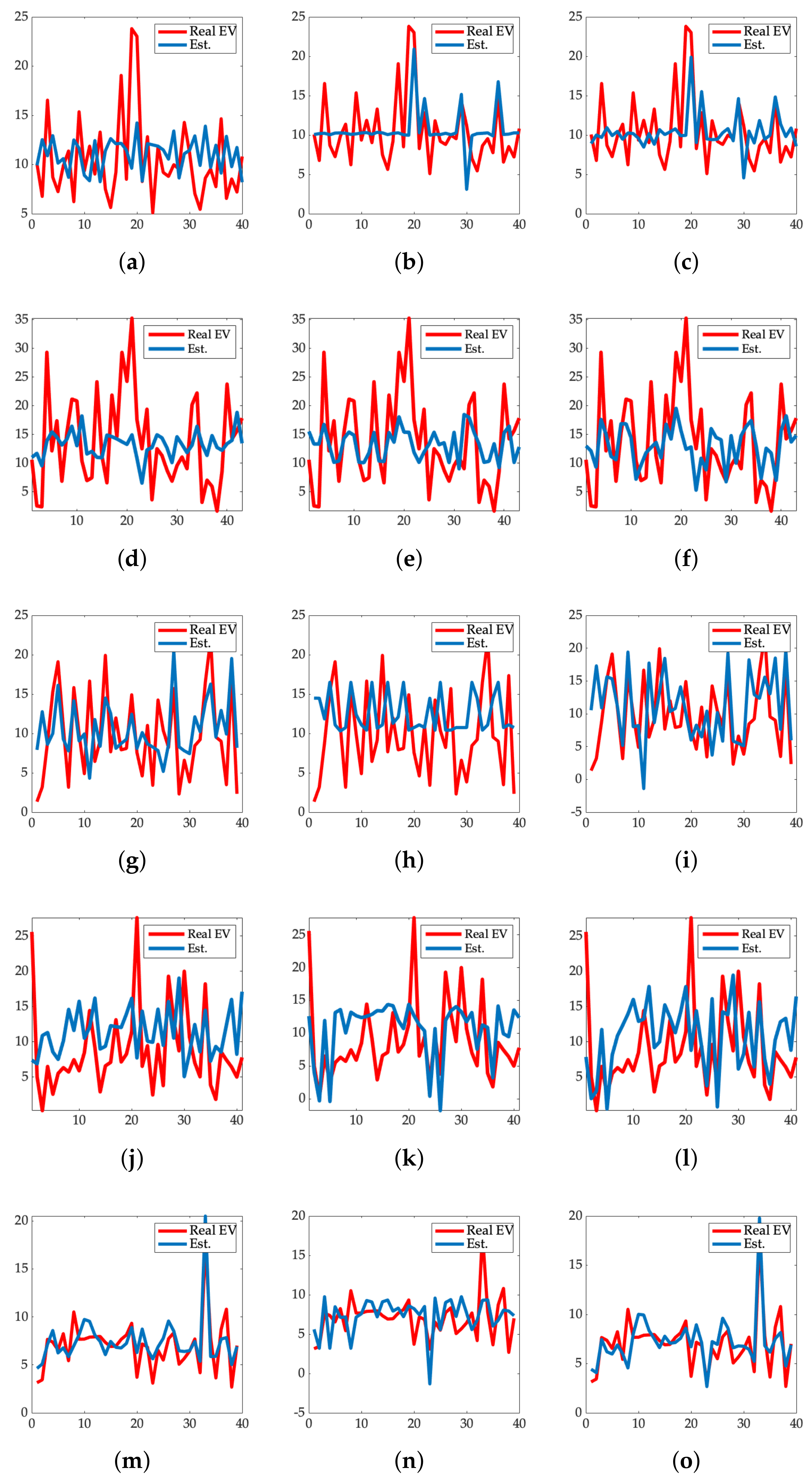
Figure 6 shows the real normalized EV values (in red) and the estimated ones (in blue). Panel (a) presents the results when incorporating as entry just the endogenous variables of the DCF valuation method. In Panel (b), the results for just the exogenous variables were considered, while Panel (c) incorporated both endogenous and exogenous as input variables for the analysis. Visual inspection of these three figures shows that estimates on Panel (c) better tacked the real valuations. In a second level, estimates on Panel (a) also followed up the real values to a certain extent, while the estimated EV only based on exogenous variables on Panel (b) resulted in the worst model, as expected. These visual results are consistent with expectations in all settings as the incorporation of exogenous information was supplying the model with additional prediction capabilities.

Table 10. Estimated EV errors by linear regression.

Variables	MSE	RMSE	MAE	${\mathbf{R}}^2$
Endogenous	48.89	6.99	4.93	0.17
Exogenous	52.53	7.24	4.24	0.10
Endogenous and Exogenous	42.50	6.51	4.49	0.28

shows the estimated figures of merit (MSE, MAE, and RMSE) for EV accuracy in linear regression for the implemented methods described earlier. Statistical error figures supported the visual inspection findings, offering better results for the model that incorporates the endogenous and exogenous variables simultaneously. In particular, lower error was obtained when considering both sets of variables, showing a RMSE of 6.51.

Figure 6 and

Table 11. Coefficients from linear regression model.

Variables	Coefficients	Estimate	pValue
Endogenous	(Intercept)	10.9898	3.20 × 10${}^{-129}$
	$\left(FC{F}_n\right)/EBITDA$	0.5794	0.1240
	$\left(FC{F}_{n-1}\right)/EBITDA$	−0.6179	0.1170
	$\left(FC{F}_{n-2}\right)/EBITDA$	−0.7975	0.0626
	$\left(FC{F}_{n-3}\right)/EBITDA$	0.4280	0.3091
	$\left(FC{F}_{n-4}\right)/EBITDA$	0.4369	0.3211
	$\left(FC{F}_{n-5}\right)/EBITDA$	1.1332	0.0058
	$(N.Debt)/EBITDA$	2.1388	1.43 × 10${}^{-07}$
Exogenous	(Intercept)	10.9898	2.16 × 10${}^{-124}$
	WACC	1.8927	0.0002
	RIR	−1.9801	1.42 × 10${}^{-06}$
	CPI	−0.8046	0.1171
	GDP	0.5356	0.2104
Endogenous and Exogenous	(Intercept)	10.9898	5.16 × 10${}^{-139}$
	$\left(FC{F}_n\right)/EBITDA$	0.7049	0.0478
	$\left(FC{F}_{n-1}\right)/EBITDA$	−0.2783	0.4537
	$(FC{F}_{(}n-2))/EBITDA$	−0.6622	0.0981
	$\left(FC{F}_{n-3}\right)/EBITDA$	0.5440	0.1662
	$(FC{F}_{(}n-4))/EBITDA$	0.5488	0.1822
	$\left(FC{F}_{n-5}\right)/EBITDA$	0.9802	0.0110
	$(N.Debt)/EBITDA$	2.6698	1.83 × 10${}^{-11}$
	WACC	2.3151	1.19 × 10${}^{-06}$
	RIR	−1.7905	1.72 × 10${}^{-06}$
	CPI	−0.5337	0.2596
	GDP	0.6064	0.1161

shows the results of the linear regression modeling coefficients with the relationship among parameters (endogenous and exogenous variables) and the valuation itself. In the first method including only the endogenous variables, the last FCF, together with the actual debt, were the most influencing parameters in EV, whilst, when considering both spectra of variables, the most influencing ones were FCF, GDP, and WACC. The results obtained here are consistent with theoretical concepts experienced earlier and published in the literature.

Figure 7 and

Table 12. Estimated EV errors with linear regression by sector.

	Errors by Sector	Cons. Cyclicals				Cons. Non-Cyclicals				Industrials				Technology				Utilities
Variables		MAE	MSE	RMSE	${\mathit{R}}^2$	MAE	MSE	RMSE	${\mathit{R}}^2$	MAE	MSE	RMSE	${\mathit{R}}^2$	MAE	MSE	RMSE	${\mathit{R}}^2$	MAE	MSE	RMSE	${\mathit{R}}^2$
Endogenous		3.77	20.82	4.56	0.21	6.89	33.30	5.77	0.17	3.56	32.19	5.67	0.41	6.94	73.72	8.59	0.50	1.23	1.53	1.24	0.81
Exogenous		3.53	20.30	4.51	0.20	5.33	27.19	5.21	0.30	7.51	38.05	6.17	0.28	6.36	130.14	11.41	0.08	2.15	5.50	2.34	0.28
Endogenous and Exogenous		3.30	17.42	4.17	0.37	6.14	24.53	4.95	0.41	4.61	24.82	4.98	0.57	6.83	71.96	8.48	0.53	1.22	1.38	1.17	0.83

show the results and the statistical analysis, respectively, for EV estimation by sector. Utilities sector was confirmed to be the most accurately followed by the deployed model, with an RMSE of 1.1746 being the smallest one. This fact was visually verified in Panels (m,n,o). In these specific companies, the estimated EV (in blue) and real EV (in red) drew closer to each other than other represented sectors, and it was especially remarkable when endogenous and exogenous variables were simultaneously used, see Panel (o).

4. Discussion and Conclusions

All the previously presented results enable us to conclude that it is not possible to develop effectively an unbiased company-valuation model by leveraging exclusively on endogenous references, for a specific market-region, sector, company, or year, and by using the different proposed DCF models with different FCF forecasting strategies. One key restriction is the lack of generalized consensus of the application of an effective closed form to obtain a discount rate WACC and its corresponding constituents that can fit the real company valuation in stock markets. With respect to the WACC analysis performed in this paper through the Inverse Method and direct approach for individual companies, although offering relevant findings, it does not allow us to justify the existence of a single value of WACC under a global perspective, and either from the sector, region, or year perspectives. Additionally, two relevant conclusions arise from this analysis: First, FCF forecasting strategies using polynomial fitting are consistently offering better results in modeling companies’ valuation; second, it is possible to obtain a WACC that fits every single company and year, and this figure could eventually be persistent in certain companies over the years.

Earlier results were evidenced to be improved by further analysis incorporating not only endogenous, but also exogenous information as drivers of external market and business environment trends, and using simple statistical learning methods, specifically linear regression. We found that the MSE and the MAE showed higher magnitudes in the valuations. Better results were obtained through a double normalization of input space, namely a statistical description with zero mean and unit STD, and a standardization (operation-oriented normalization). In particular, input space operative normalization, and the statistical normalization in a lower extent, enhance the generalization capabilities by making them independent from volume or currency. Regression analysis with only endogenous variables obtained a RMSE of 6.99, whereas when exogenous variables were incorporated to the input space variability is improved, RMSE was reduced to 6.51, and the determination coefficient $R^2$ reached 0.28.

Hence, we can conclude from the results obtained that the operational variables and models evaluated in this work have been validated from an intrinsic valuation capabilities perspective, as it is viable to set the free parameters to match stock market pricing. Additionally, and in order to validate a systematic and unbiased model for companies’ valuation, we required supplementary exogenous variables complementing the historical financial statements, which can incorporate general market trends and investor business expectations. Furthermore, the application of simple statistical learning techniques for a bundled analysis boosted the results and performance.

The main contributions of this work could be considered in three directions. First, although we did not obtain statistically significance in specific cases, the implementation of the Inverse Method to estimate WACC across markets and industries can offer an alternative systematic tool for value assessment. Furthermore, we consider that the information obtained as a result of this effort could constitute additional valid features to be used in advanced valuation models using ML methods. Second, the published reference WACCs are hardly applicable in reality to accurately match market expectation, but offers a valid representation of global market expectation that again could be considered as part of the input space for applications beyond traditional approaches. Finally, as a first step toward a later in-depth study leveraging on ML methods presented in the companion paper, a linear regression scheme is introduced, with or without exogenous variables. This last analysis is carried out incorporating not only straight from the financial reports accounting data, but also the features obtained in the previous experiments. We expect that these three key findings pave the way toward more sophisticated developments in the valuation field. Therefore, we propose a deeper analysis of ML techniques in the companion paper [49], leveraging on the valid results and conclusions of the present work.

References

1. Koller, T.; Goedhart, M.; Wessels, D. Valuation: Measuring and Managing the Value of Companies, 15th ed.; John Wiley & Sons, Inc.: Hoboken, NJ, USA, 2010. [Google Scholar]
2. Shapiro, E.; Mackmin, D.; Sams, G. Modern Methods of Valuation, 12th ed.; Estates Gazette: London, UK, 2019. [Google Scholar]
3. Stowe, J.; Robinson, T.; Pinto, J.; McLeavey, D. Equity Asset Valuation, 4th ed.; John Wiley & Sons, Inc.: Hoboken, NJ, USA, 2015. [Google Scholar]
4. Fabozzi, F.J.; Focardi, S.M.; Jonas, C. Equity Valuation: Science, Art, or Craft? 1st ed.; CFA Institute Research Foundation Publications: Chicago, IL, USA, 2017. [Google Scholar]
5. Stickney, C.; Weil, R.L.; Schipper, K. Financial Accounting: An Introduction to Concepts, Methods And Uses, 14th ed.; Cengage Learning: Boston, MA, USA, 2014. [Google Scholar]
6. Zmijewski, M.E. Methodological issues related to the estimation of financial distress prediction models. J. Account. Res. 1984, 22, 59–82. [Google Scholar] [CrossRef]
7. Mnejja, A.; Sahut, J.M. The discount premium between private M&A and LBO transactions. Nous 2010, 19, 20–47. [Google Scholar]
8. Blume, L.; Easley, D.; O’hara, M. Market statistics and technical analysis: The role of volume. J. Financ. 1994, 49, 153–181. [Google Scholar] [CrossRef]
9. Allen, H.; Taylor, M.P. Charts, noise and fundamentals in the London foreign exchange market. Econ. J. 1990, 100, 49–59. [Google Scholar] [CrossRef]
10. Damodaran, A. Damodaran on Valuation: Security Analysis for Investment and Corporate Finance, 2nd ed.; John Wiley & Sons, Inc.: Hoboken, NJ, USA, 2016; Volume 324. [Google Scholar]
11. Shynkevich, A. Performance of technical analysis in growth and small cap segments of the US equity market. J. Bank. Financ. 2012, 36, 193–208. [Google Scholar] [CrossRef]
12. Menkhoff, L. The use of technical analysis by fund managers: International evidence. J. Bank. Financ. 2010, 34, 2573–2586. [Google Scholar] [CrossRef] [Green Version]
13. Colby, R.W.; Meyers, T.A. The Encyclopedia of Technical Market Indicators, 2nd ed.; McGraw-Hill Companies, Inc.: New York, NY, USA, 2002. [Google Scholar]
14. Graham, B.; Dodd, D. Security Analysis: Principles and Techniques, 2nd ed.; McGraw-Hill Companies, Inc.: New York, NY, USA, 1934. [Google Scholar]
15. Edwards, R.D.; Magee, J.; Bassetti, W.C. Technical Analysis of Stock Trends, 11th ed.; CRC Press: Boca Raton, FL, USA, 2018. [Google Scholar]
16. Williams, J.B. The Theory of Investment Value; Harvard University Press: Cambridge, MA, USA, 1938. [Google Scholar]
17. Ochoa Ramírez, S.A.; Toscano Moctezuma, J.A. Revisión crítica de la literatura sobre el análisis financiero de las empresas. Nóesis: Revista de Ciencias Sociales y Humanidades 2012, 21, 73–100. [Google Scholar] [CrossRef] [Green Version]
18. Valls Martínez, M.d.C. Métodos clásicos de valoración de empresas. Investigaciones Europeas de Dirección y Economía de la Empresa 2001, 7, 49–66. [Google Scholar]
19. Kim, S.; Ku, S.; Chang, W.; Song, J.W. Predicting the Direction of US Stock Prices Using Effective Transfer Entropy and Machine Learning Techniques. IEEE Access 2020, 8, 111660–111682. [Google Scholar] [CrossRef]
20. Fernandez Arjona, L.; Filipović, D. A machine learning approach to portfolio pricing and risk management for high-dimensional problems. Swiss Financ. Inst. Res. Pap. 2020, 1, 20–28. [Google Scholar]
21. Choudhry, R.; Garg, K. A hybrid machine learning system for stock market forecasting. World Acad. Sci. Eng. Technol. 2008, 39, 315–318. [Google Scholar]
22. Nelson, D.M.; Pereira, A.C.; de Oliveira, R.A. Stock market’s price movement prediction with LSTM neural networks. In Proceedings of the 2017 International joint conference on neural networks (IJCNN), Anchorage, AK, USA, 14–19 May 2017; pp. 1419–1426. [Google Scholar]
23. Fernández, P. Métodos de valoración de empresas (Company Valuation Methods). SSRN Electron. J. 2017, 1, 1–28. [Google Scholar]
24. Fernández, P. A More Realistic Valuation: APV and WACC with Constant Book Leverage Ratio; Working Paper 715; IESE Business School: Barcelona, Spain, 2007. [Google Scholar]
25. Graham, B. The Intelligent Investor, 4th ed.; Harper Collins: New York, NY, USA, 1984. [Google Scholar]
26. Vidal, R.; Ribal, J. Valuation of agrifood SMEs. Lessons to be learnt from the stock market. Span. J. Agric. Res. 2017, 15, 1–15. [Google Scholar] [CrossRef]
27. Liu, J.; Nissim, D.; Thomas, J. Equity valuation using multiples. J. Account. Res. 2002, 40, 135–172. [Google Scholar] [CrossRef]
28. Olbrich, M.; Quill, T.; Rapp, D.J. Business valuation inspired by the Austrian school. J. Bus. Valuat. Econ. Loss Anal. 2015, 10, 1–43. [Google Scholar] [CrossRef]
29. Bruner, R.F.; Eades, K.M.; Harris, R.S.; Higgins, R.C. Best practices in estimating the cost of capital: Survey and synthesis. Financ. Pract. Educ. 1998, 8, 13–28. [Google Scholar]
30. Fernández, P. Valuation Methods and Shareholder Value Creation, 1st ed.; Academic Press: Orlando, FL, USA, 2002. [Google Scholar]
31. Damodaran, A. Applied Corporate Finance, 3rd ed.; John Wiley & Sons, Inc.: New York, NY, USA, 2010. [Google Scholar]
32. Liu, J.; Nissim, D.; Thomas, J. Is cash flow king in valuations? Financ. Anal. J. 2007, 63, 56–68. [Google Scholar] [CrossRef] [Green Version]
33. Dechow, P.M.; Hutton, A.P.; Sloan, R.G. An empirical assessment of the residual income valuation model. J. Account. Econ. 1999, 26, 1–34. [Google Scholar] [CrossRef]
34. Francis, J.; Olsson, P.; Oswald, D.R. Comparing the accuracy and explainability of dividend, free cash flow, and abnormal earnings equity value estimates. J. Account. Res. 2001, 38, 45–70. [Google Scholar] [CrossRef] [Green Version]
35. Plenborg, T.; Pimentel, R.C. Best practices in applying multiples for valuation purposes. J. Priv. Equity 2016, 19, 55–64. [Google Scholar] [CrossRef]
36. Jiang, X.; Lee, B.S. An empirical test of the accounting-based residual income model and the traditional dividend discount model. J. Bus. 2005, 78, 1465–1504. [Google Scholar] [CrossRef]
37. Campbell, J.Y.; Vuolteenaho, T. Bad beta, good beta. Am. Econ. Rev. 2004, 94, 1249–1275. [Google Scholar] [CrossRef] [Green Version]
38. Fischer, T.; Krauss, C. Deep learning with long short-term memory networks for financial market predictions. Eur. J. Oper. Res. 2018, 270, 654–669. [Google Scholar] [CrossRef] [Green Version]
39. Krauss, C.; Do, X.A.; Huck, N. Deep neural networks, gradient-boosted trees, random forests: Statistical arbitrage on the S&P 500. Eur. J. Oper. Res. 2017, 259, 689–702. [Google Scholar]
40. Martin, A.; Manjula, M.; Venkatesan, P. A business intelligence model to predict bankruptcy using financial domain ontology with association rule mining algorithm. IJCSI Int. J. Comput. Sci. Issues 2011, 259, 689–702. [Google Scholar]
41. Moreno, J.F.; Melo, L.F. Pronóstico de incumplimientos de pago mediante máquinas de vectores de soporte: Una aproximación inicial a la gestión del riesgo de crédito. Borradores de Economía 2011, 677, 1–32. [Google Scholar]
42. Huang, W.; Nakamori, Y.; Wang, S.Y. Forecasting stock market movement direction with support vector machine. Comput. Oper. Res. 2005, 32, 2513–2522. [Google Scholar] [CrossRef]
43. Hernandez-Perdomo, E.; Guney, Y.; Rocco, C.M. A reliability model for assessing corporate governance using machine learning techniques. Reliab. Eng. Syst. Saf. 2019, 185, 220–231. [Google Scholar] [CrossRef]
44. Moro Visconti, R.; Montesi, G.; Papiro, G. Big data-driven stochastic business planning and corporate valuation. Corp. Ownersh. Control. 2018, 15, 189–204. [Google Scholar] [CrossRef]
45. Soguero-Ruiz, C.; Gimeno-Blanes, F.J.; Mora-Jiménez, I.; Martínez-Ruiz, M.P.; Rojo-Álvarez, J.L. On the differential benchmarking of promotional efficiency with machine learning modeling (I): Principles and statistical comparison. Expert Syst. Appl. 2012, 39, 12772–12783. [Google Scholar] [CrossRef]
46. Melgarejo-Meseguer, F.M.; Gimeno-Blanes, F.J.; Salar-Alcaraz, M.E.; Gimeno-Blanes, J.R.; Martínez-Sánchez, J.; García-Alberola, A.; Rojo-Álvarez, J.L. Electrocardiographic Fragmented Activity (II): A Machine Learning Approach to Detection. Appl. Sci. 2019, 9, 3565. [Google Scholar] [CrossRef] [Green Version]
47. Arnold, G.; Davies, M. Value-Based Management: Context and Application, 1st ed.; John Wiley & Sons, Inc.: Chichester, UK, 2000. [Google Scholar]
48. Nissim, D. Relative valuation of U.S. insurance companies. Rev. Account. Stud. 2013, 18, 324–359. [Google Scholar] [CrossRef]
49. Vayas-Ortega, G.; Soguero-Ruiz, C.; Rojo-Álvarez, J.L.; Javier, G.B.F. On the Differential Analysis of Enterprise Valuation Methods as a Guideline for Unlisted Companies Assessment (II): Applying Machine Learning Techniques for Unbiased Enterprise Value Assessment. Appl. Sci. 2020, 15, 5334. [Google Scholar] [CrossRef]
50. Gunn, S. Support Vector Machines for Classification and Regression; Technical Report 1, ISIS Technical Report; University of Southampton: Southampton, UK, 1998. [Google Scholar]
51. Eikon, T.R. Electronic Global Equity Data Base from Eikon Thomson Reuters. Available online: https://eikon.thomsonreuters.com/index.html (accessed on 31 March 2018).
52. Group, T.W.B. World Bank National Accounts Data, and OECD National Accounts Data Files. Available online: https://data.worldbank.org/indicator/ny.gdp.mktp.cd (accessed on 7 August 2018).
53. Martinez, W.L.; Martinez, A.R.; Solka, J. Exploratory Data Analysis with MATLAB, 2nd ed.; CRC Press: London, UK, 2017. [Google Scholar]
54. Arumugam, T.T. An analysis of discounted cash flow (DCF) approach to business valuation in Sri Lanka. Ph.D. Thesis, St Clements University, Colombo, Sri Lanka, 2007. [Google Scholar]
55. Michelfelder, R.A. Empirical analysis of the generalized consumption asset pricing model: Estimating the cost of capital. J. Econ. Bus. 2015, 80, 37–50. [Google Scholar] [CrossRef]
56. Samonas, M. Financial Forecasting, Analysis, and Modelling: A Framework for Long-Term Forecasting, 3rd ed.; John Wiley & Sons, Inc.: Chichester, UK, 2015. [Google Scholar]
57. Fernández, P. WACC: Definition, misconceptions, and errors. Bus. Valuat. Rev. 2010, 29, 138–144. [Google Scholar] [CrossRef]
58. Koller, T.; Goedhart, M.; Wessels, D.; Benrud, E. Valuation Workbook: Step-by-step Exercises and Tests to Help You Master Valuation; John Wiley & Sons: Hoboken, NJ, USA, 2011; Volume 496. [Google Scholar]
59. Murphy, K.P. Machine Learning: A Probabilistic Perspective, 1st ed.; MIT press: London, UK, 2012. [Google Scholar]
60. Ayodele, T.O. Types of machine learning algorithms. New Adv. Mach. Learn. 2010, 3, 19–48. [Google Scholar]
61. Montgomery, D.C.; Peck, E.A.; Vining, G.G. Introduction to Linear Regression Analysis; John Wiley & Sons: Hoboken, NJ, USA, 2012; Volume 821. [Google Scholar]
62. Fernández, P. Company valuation methods. The most common errors in valuations. IESE Bus. Sch. 2007, 449, 1–27. [Google Scholar] [CrossRef] [Green Version]
63. Chazalon, P.; Maréchal, A.; Bard, F.; Joulié, A. Access to standardized WACC calculations. Available online: http://www.waccexpert.com (accessed on 18 May 2018).
64. Damodaran, A. Cost of Capital by Sector—Multiple Data Services. Available online: http://people.stern.nyu.edu/adamodar/New_Home_Page/datafile/wacc.htm (accessed on 20 July 2020).
65. Weiss, S.M.; Kapouleas, I. An empirical comparison of pattern recognition, neural nets, and machine learning classification methods. IJCAI 1989, 89, 781–787. [Google Scholar]
66. Liu, H.; Cocea, M. Semi-random partitioning of data into training and test sets in granular computing context. Granul. Comput. 2017, 2, 357–386. [Google Scholar] [CrossRef] [Green Version]
Figure 1. Effective WACC (in%) obtained with the inverse method and for the five different implemented valuation models for 3MCo in 1992, using the NPV calculation described in Equation (5).
Applsci 10 05875 g001
Figure 2. Effective WACCs for several years (x axis) and companies (y axis) obtained by the inverse method and EV models: (a) M1, (b) M2, (c) M3, (d) M4, (e) M5.
Applsci 10 05875 g002
Figure 3. Bar graph of frequency of WACCs for sectors: (a) Consumer Cyclicals; (b) Consumer non-Cyclicals; (c) Industrial; (d) Technology; (e) Utilities.
Applsci 10 05875 g003
Figure 4. Bar graph of frequency of effective WACCs for market regions: (a) Brazil, (b) India, (c) Japan, (d) United States, (e) Spain.
Applsci 10 05875 g004
Figure 5. Errors for several years (x axis) and companies (y axis) obtained when considering the reference WACC in the EV models: (a) M1, (b) M2, (c) M3, (d) M4, (e) M5.
Applsci 10 05875 g005
Figure 6. Actual estimated EV using (a) endogenous, (b) exogenous, (c) endogenous and exogenous variables.
Applsci 10 05875 g006
Figure 7. EV estimated by sector. Reading from top to bottom, we find Panels (ac) for Consumer Cyclicals; (df) for Consumer Non- Cyclicals; (gi) for Industrial; (jl) for Technology, and (mo) for Utilities. Reading from left to right, we have endogenous, exogenous, and endogenous and exogenous variables in the input space.
Applsci 10 05875 g007