1. Introduction
The escalator is one of the most popular transportation vehicles in densely populated areas. According to the data, almost 2 billion trips are taken using elevators and escalators every day. Once escalator failure occurs, it may lead to a terrible accident [
1]. In China, about 40 persons died and thousands of people were injured in escalator accidents every year. According to data statistics from Guangzhou Metro, about 67% of total injuries are escalator-related injuries [
2]. Thus, the timely prediction of escalator failure can help the manager and maintenance personnel develop maintenance plans to effectively prevent accidents.
The escalator is a typical human–machine–environment system with many factors involved in safety. One of the links and one personal mistake may cause a serious accident. As a research field related to people’s transportation, safety issues have always been the focus of attention [
3,
4,
5]. An escalator, as a complex system, can cause serious casualties in the event of malfunction. Therefore, the safe operation of escalators deserves in-depth study. Failure and risk prediction are critical to ensuring the safe operation of escalators. When the risk level exceeds a certain safety range, an accident will occur [
6]. Thus, it is necessary to predict the failure time accurately and timely, and arrange maintenance activities in advance, which can effectively reduce the failure rate and reduce accidents. Failure time series modeling analysis can describe the law of failure occurrence by establishing a corresponding mathematical model of related failure data.
Many scholars have done in-depth research on time series analysis in safety research, such as failure maintenance time based on the Weibull distribution [
7], shipyard occupational risk assessment based on multivariate regression and genetic algorithm [
8], and the Akaike Information Criterion (AIC) based steel mill alarm mechanism [
9]. These methods have achieved good effects in the case of large amounts of data. However, for accident-related failure data, it has special features of short samples, non-uniform sampling, and random interference. Traditional data modeling based on statistical laws or deterministic mathematical models requires more labelled data, while data related to safety accidents have typical characteristics as aforementioned, making data modeling problems much more difficult. Neural network technology, as one of the most popular data analysis methods, can build a model containing complex nonlinear relationships without deliberate attention to the mathematical characteristics of the data itself, and has good generalization ability to map the relationship between input and output quickly and effectively, which has been widely used in many fields.
In recent years, with the development of neural network (NN) technology, neural networks have been used in various fields [
10,
11,
12]. The data modeling by NNs does not deliberately focus on the mathematical characteristics of the data itself but learns to construct the complex relationship between input and output with neurons. Thus, neural networks have good generalization capacity. However, the accuracy of neural networks is sensitive to disturbance in data. In addition, some neural networks only pay attention to the relationship between input and output, ignoring the hidden information of the input themselves, which is unreasonable for time series modeling and prediction. Long short-term memory (LSTM), as one of the recurrent neural networks (RNNs), was proposed to solve the problem of time series prediction [
13]. LSTM can analyze and process time series with unknown duration delay. LSTM can improve the memory module of traditional RNNs and avoid the problem where effective historical information cannot be stored for a long time, because of the constant input data [
14]. LSTM has also been utilized in time series prediction [
15], remaining useful for life prediction [
16] and safety analysis [
17,
18]. However, LSTM does not learn well the characteristics of the data itself for short time series with too few samples. Therefore, this paper considers the short-sequence feature extraction ability of a convolutional neural network (CNN) to extract high-dimensional features, which can help the LSTM unit to understand the data better. In addition, the combination of CNNs and LSTMs in a unified framework has already offered state-of-the-art results in the speech recognition domain [
19], health care [
20], and power load prediction [
21]. In addition, the quality of the data itself makes a big difference to the accuracy of neural network modeling. Meanwhile, considering the short length and random interference in the failure data, it is meaningful to enhance the data quality to improve the prediction accuracy of the neural network before data modeling. Dynamic time warping (DTW) [
22], with characteristics of oversampling and similarity matching, is much more suitable for data preprocessing before data modeling, especially for short and interfering failure data. DTW has also been used in many fields [
23,
24]. For this reason, considering the above-mentioned issues, a new failure time series prediction method for the escalator based on a convolutional long short-term memory neural network combined with dynamic time warping preprocessing (DCLNN) was proposed in this paper.
The remainder of this paper is organized as follows: In
Section 2, a time series with high stationarity and low complexity is elected by a comprehensive selection indicator, the main principles of the DCLNN are given, and the diagram of the proposed method for failure time prediction is described. In
Section 3, case studies of six escalators are applied with the proposed method and the results are given. Finally, a summary and conclusion are drawn in
Section 4.
2. The Proposed DCLNN Method for Failure Time Prediction
The complex working environment and numerous components of the escalator make the failure time data have typical nonlinearity and randomness, which increases the difficulty of data modeling of the escalator failure time series. In this section, an escalator failure time prediction model based on a deep neural network under dynamic time warping preprocessing (DCLNN) will be specifically explained. The DCLNN combined the strategy of DTW pre-processing and CNNLSTM post-learning, and some basic principles about the method are given in the following section.
2.1. The DCLNN Strategy for Failure Time Prediction of Escalator
The accuracy of time series prediction is not only related to the sequence model, but the quality of the time series itself also has a great influence on the prediction result. In this paper, a strategy to combine data quality enhancement with deep neural networks is proposed for time series prediction, which is shown in
Figure 1. First, the data sequences are divided into good data and bad data according to a selection indicator; secondly, the bad time series data can be transformed to good data with high quality; finally, the built neural network is used to train and predict the time series.
Based on the principles of DTW and CNNLSTM, a time series prediction method combining DTW pre-processing and CNNLSTM post-learning is proposed in this paper for escalator failure time prediction, which is called DCLNN.
2.2. Comprehensive Selection Indicator before Data Modeling
In general, data sequences with high stationarity and low complexity can be modeled accurately by the behavior of mathematical modeling. The failure time has certain statistical rules, but with various reasons for failure, different escalators have different failure times. Those regular escalators whose failure time series are stationary and have lower complexity can be selected as a reference. For the same batch of equipment, other escalators have similar failure occurrence rules. In this paper, two stationary indicators (SIs) and two complexity indicators (CIs) are combined to form a comprehensive selection indicator to select excellent referenced time series. Here are details about four indicators:
(1) Stationary indicator
In statistics, the standard deviation is a measure that is used to quantify the amount of variation or dispersion of a set of data values. A low standard deviation indicates that the time series tends to be more stationary.
(b) p-value
The
p-value is the probability value in the statistical significance test, that is, the probability that the hypothesis test occurs. It is generally assumed that if a small probability event occurs, the assumption is true. In this paper, the data sequence is used as the hypothesis test for the stationary data, and the P-value can be calculated as the probability of the unit root test to judge whether the failure time series is stationary or not. A low P-value indicates that the time series tends to be stationary.
(2) Complexity indicator
(a) Lempel-ziv
The Lempel-ziv indicator is used to characterize the rate at which new patterns appear in a time series. The higher the Lempel-Ziv complexity of the sequence, the greater the degree to which the signal sequence is near-random. The lower the Lempel-ziv indicator, the lower the complexity of the time series.
is the Lempel-ziv complexity of the time series, and
is the normalized complexity. Details about the Lempel-ziv algorithm can be found in Ref. [
25].
(b) Sample entropy
The Sample Entropy (SampEn) measures the complexity of the time series by measuring the probability of generating a new pattern in the signal. The greater the probability of the new pattern, the greater the complexity of the sequence. The lower the sample entropy indicator, the lower the complexity of the time series.
where
and
are the number of subsets of the original time series that satisfies the requirement within the similar distance
(usually
).
(3) Comprehensive selection indicator
In order to describe the inherent characteristics of a data sequence, a comprehensive selection indication (CSI) that can describe both stationarity and complexity is constructed in this part to select an inherently excellent data sequence before data modeling. In addition, CSI can be given by the following equation:
CSI can be used to compare the regularity itself between data sequences; the smaller the CSI, the better the data sequence itself and the more accurate the data modeling will be.
2.3. Dynamic Time Warping
The failure time series of escalators are different, and the raw data always have defects (such as disturbances), which are less effective when used directly in the prediction of neural networks. Considering the time delay and local similarity of the failure time series of different escalators, dynamic time warping (DTW) is introduced to pre-process before data modeling [
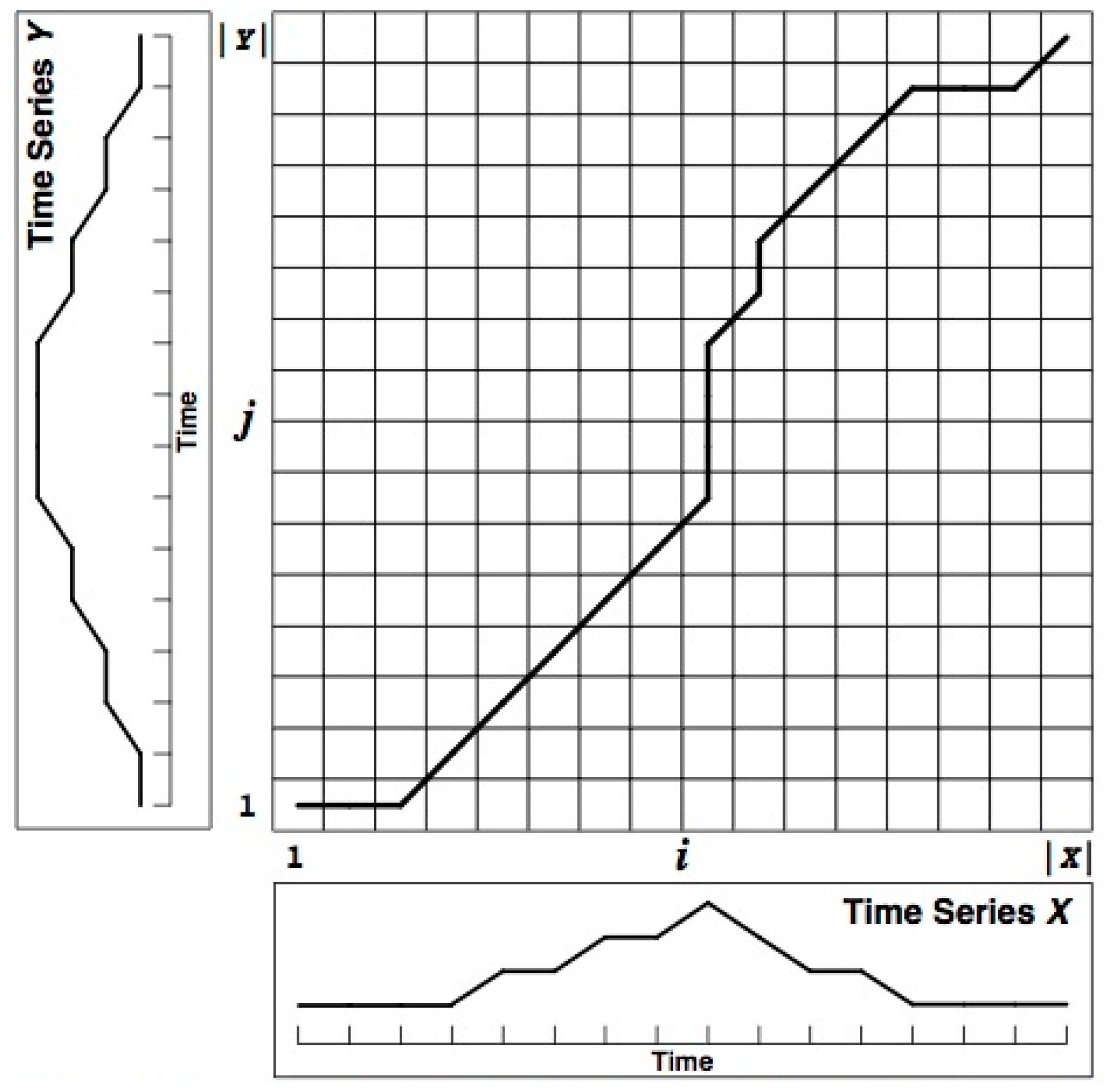
22], and the over-sampling characteristics of data under the space defined by DTW can effectively reduce the impact of the mutated data on the accuracy of the model while increasing the data capacity and finally improve the prediction accuracy of the NN model. An intuitive example is given in
Figure 2. The principles of DTW can be further explained as follows:
Given two time series
and
, whose lengths are, respectively,
and
, the warping path can be given,
The warping path
must start from
and end with
to ensure every coordinate in
and
would be considered. Besides, the coordinate
and
in
of the warping path must be monotonically increasing, which can be constrained by the following equation
The warping path needs to satisfy continuity and monotonicity. According to this, Equation (8) represents the three directions that are in the next optimal path searching. This process can be shown in
Figure 3. DTW always searches forward for the closest distance in three directions: Horizontal, vertical, and diagonal upward, to maintain the continuity and monotonicity.
For the failure time of the escalator, such a warping path in DTW is physically meaningful. No new values will be added to the original data after DTW with the reference time series.
Finally, the wanted warping path is the shortest path in all possible warping paths
DTW is a typical optimization problem. It uses a time warping function that satisfies certain conditions to describe the time correspondence between the test template and the reference template, and solves the warping function corresponding to the minimum cumulative distance when the two templates match. In addition, the constraint here is the search direction shown in
Figure 3 [
26]. DTW always searches forward for its nearest distance from three directions: Horizontal direction, vertical direction, and diagonal upward direction. These three directions are consistent with the basic law of the failure time series: (i) The horizontal direction indicates the same failure time; (ii) the vertical direction indicates sudden failure; (iii) the diagonal line indicates the stable development direction of the failure time. It is this constraint that allows the warping time series to learn the inherent failure development information of ‘good data’ while maintaining the original basic physical meaning of itself. Meanwhile, for short time series prediction, DTW can increase the sample capacity for its oversampling characteristics, especially to increase the sample capacity where the data are abrupt, so that the modeling of the disturbance in the neural network can obtain more attention to reduce the influence of disturbance to the whole data model.
2.4. Convolutional LSTM Neural Network
The significant characteristic of the failure time series in this paper is a few samples with non-uniform sampling. When directly using LSTM for data modeling, the features in time series are not obvious, which may lead to poor accuracy of the modeling and prediction. The deep neural network used in this paper is a combination of CNN and LSTM. The main target of this paper is time series prediction. With the help of the CNN’s feature extraction ability, high-dimensional features can be trained to understand the failure time series more comprehensively. Then, these high-dimensional features can be used for time series prediction in LSTM. Based on the advantages of CNN and LSTM, a convolutional LSTM neural network (CLNN) is proposed to achieve the goal of failure time prediction for an escalator.
2.4.1. Convolutional Neural Network
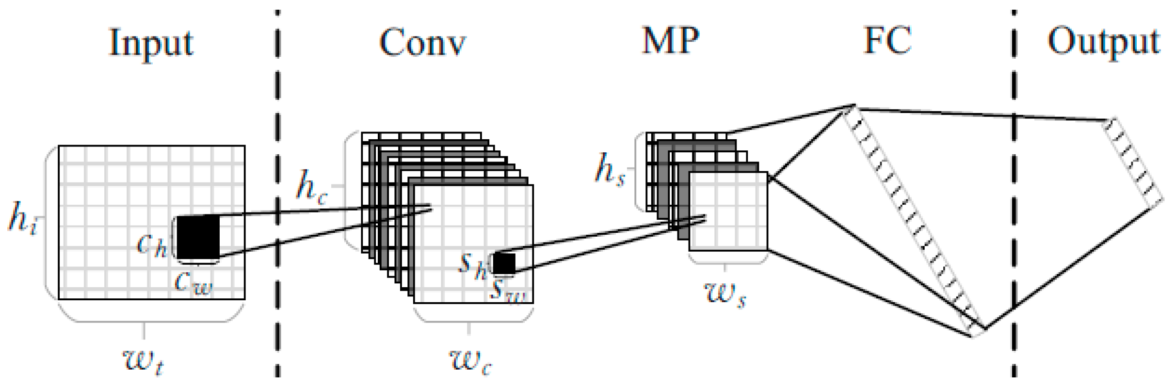
Convolutional neural networks are a type of deep neural network with the ability to act as feature extractors. Such models are able to learn multiple layers of feature hierarchies automatically (also called ‘representation learning’). A typical CNN network structure is shown in
Figure 4. This typical CNN includes an input layer, a convolution layer (Conv), a maximum pooling layer (MP), a fully connected layer (FC), and an output layer.
The structure of the CNN network mainly has two characteristics: Sparse connection and shared weights. As shown in
Figure 5, unlikely a fully connected neural network, CNNs use the locally connected mode. The neurons in the m layer are connected to the adjacent neurons in the m-1 layer. The weights of every neuron in the m-1 layer are shared to the neurons in the m layer, which means the weights with the same color in
Figure 4 are the same. Due to these advantages, the CNN has the effect of regularization, which can improve the stability and generalization ability of neural networks and avoid over-fitting. At the same time, these two advantages reduce the total amount of weight parameters, which is beneficial to the rapid learning of neural networks. CNNs have good representation learning ability, which can learn excellent features through network training. It is very suitable for a learning process lacking prior knowledge or clear features.
In this paper, the failure time in the failure recall data is a typical time series, so a one-dimensional (1D) convolution operation is used to extract the features of failure time sequences.
2.4.2. Long Short-Term Memory Neural Network
After data sequences have been preprocessed, a long short-term memory neural network (LSTM NN) is applied in this paper for data modeling. To overcome the gradient vanish of traditional RNNs, a LSTM NN was proposed. LSTM is one of the special structures of RNNs that can solve the memory problem of neural networks. It can be applied to process and predict important events with long intervals and delays in time series.
With a special gate and cell in the hidden layer, LSTM can effectively update and deliver critical information in time series. Compared to traditional RNNs, LSTM has stronger capacities of information selection and time series learning, which can solve the problem of long-term dependencies by using remote context information for current prediction tasks. An LSTM is composed of one input layer, one hidden layer, and one output layer. Unlike the traditional NN, the basic unit of the hidden layer is a memory block, and LSTM adds a ‘processor’ in the algorithm to judge whether the information is useful or not, which is called a cell [
27].
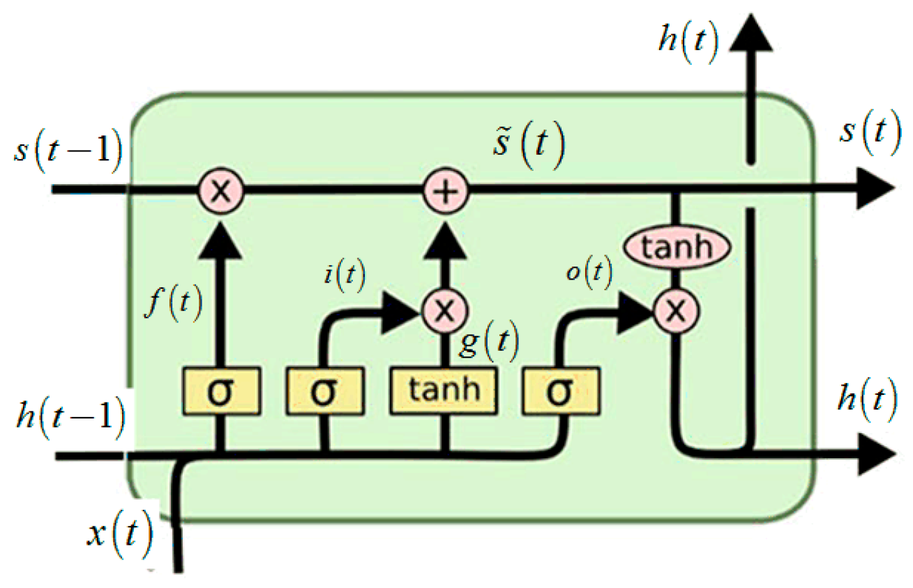
The typical structure of an LSTM cell is shown in
Figure 6. An LSTM cell is configured mainly by three gates: Input gate, forget gate, and output gate. The basic idea of LSTM is that when information enters the network, the information that meets the requirements is left by the input gate, the non-compliant information is discarded by the forget gate, and finally new information is generated by the output gate.
Given is the input time series, the output is denoted as and the memory of the cell is denoted as . Three gates of the LSTM NN can be given as follows:
(1) Forget gate
This unit is decided by considering the current input, the previous output, and the previous memory. It will produce a new output and change its memory.
determines how much information can be left.
(2) Input gate
The input of this unit is the same with the forget gate, but the input gate determines the extent to which new memories should affect old memories. Meanwhile, this unit determines how much new information should be delivered to the next cell. Finally, the cell state is updated through discarding the information that needs to be discarded and adding new information.
(3) Output gate
Based on the new cell state, some information of the new state should be added to the output and the output information of the cell will finally be determined by deterministic information that needs to be output.
where
denotes the sigmoid function defined in the equation and the
function is defined in the equation:
The learning process of LSTM mainly includes the error backpropagation process and optimization algorithm. The backpropagation through time (BPTT) algorithm is applied in the error backpropagation process of LSTM [
28].
2.4.3. CLNN: Combination of CNN and LSTM
The architecture of an CLNN is shown in
Figure 7. In addition, the network structure of an CLNN consists of a convolutional layer, a pooling layer, LSTM units, and two fully connected layers.
3. Application for Failure-Recall Data with DCLNN Method
3.1. Description of Failure-Recall Data
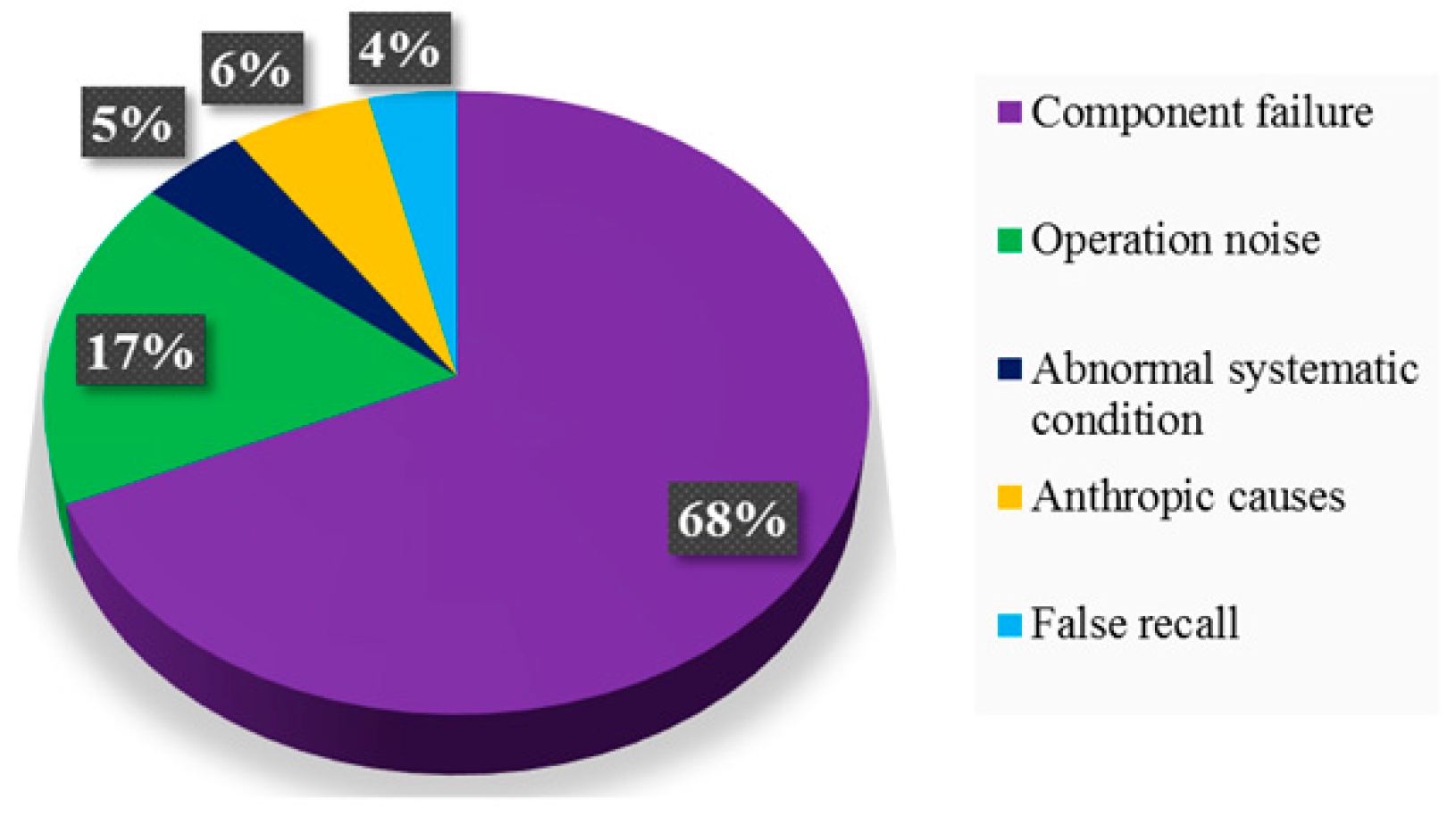
The current maintenance activities of an escalator are mainly based on two modes: Periodical maintenance and failure-recall maintenance. The maintenance of different components in periodical maintenance is carried out in different cycles (for example, the four types of maintenance items for the escalator with a cycle of 4, 12, 24, and 52 weeks). The failure-recall maintenance aims at the problems discovered by the operator to perform inspection and repair. The failure-recall record can directly reflect the operational safety of the escalator to a certain extent. The failure-recall records of six escalators during 2012.10–2018.10 are investigated. The statistics of failure-recall reasons is shown in
Figure 8. There are five main situations in which the failure is recorded, and the cause of component failure accounts for the most.
The failure of the escalator is related to the failure of the components, the time of use, and the inherent performance degradation of the system. The collection and analysis of relevant data can provide scientific predictions for escalator failure. In addition, predicting the possible time of escalator failure and implementing maintenance in advance can reduce the chance of escalator failure and reduce casualties. The failure-recall record can reflect the failure occurrence rule and safety condition of an escalator. However, data in the failure-record have the characteristics of short samples, non-uniform samplings, and random interference, which brings difficulty in predicting the failure time of an escalator.
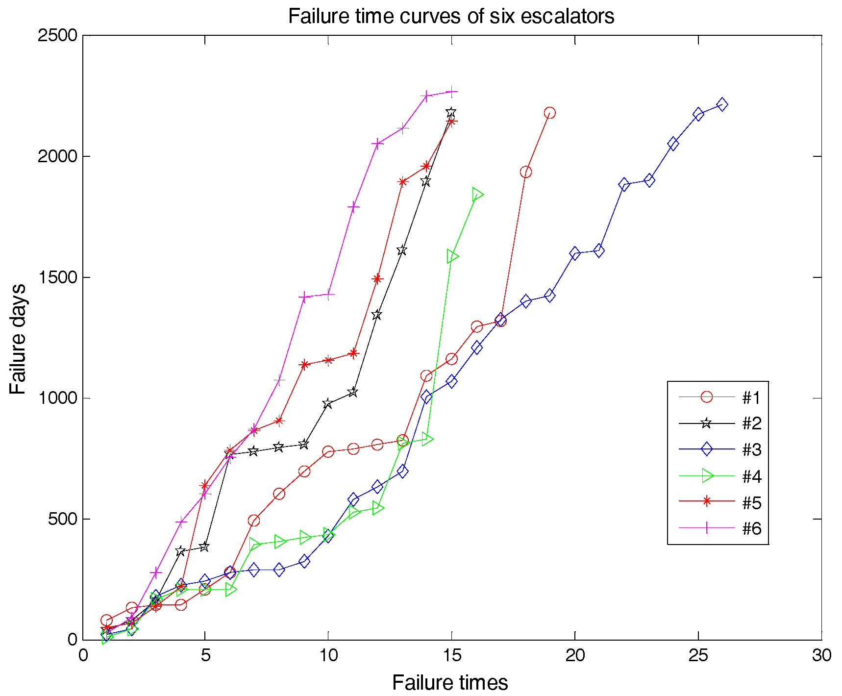
In this paper, failure-recall records of six escalators with the same brand are collected. In the records, some details about every failure time are recorded and shown in
Appendix A. Then, the failure time is processed into the corresponding failure interval days, and the failure time curves of the escalators are calculated by the accumulation idea. The processed failure time curve is shown in
Figure 9.
3.2. Dynamic Time Warping Pre-Processing Before Data Modeling
In this part, failure time datasets of different escalators are distinguished by the abovementioned indicators to find those excellent data sequences with inherent advantages (high stationarity and low complexity) before data modeling. In addition, other data sequences are matched similarly with the selected excellent data using DTW. The above process can be seen as a pre-processing for more accurate data modeling.
Table 1 summarizes the stationary indicators and complexity indicators of the original failure time series.
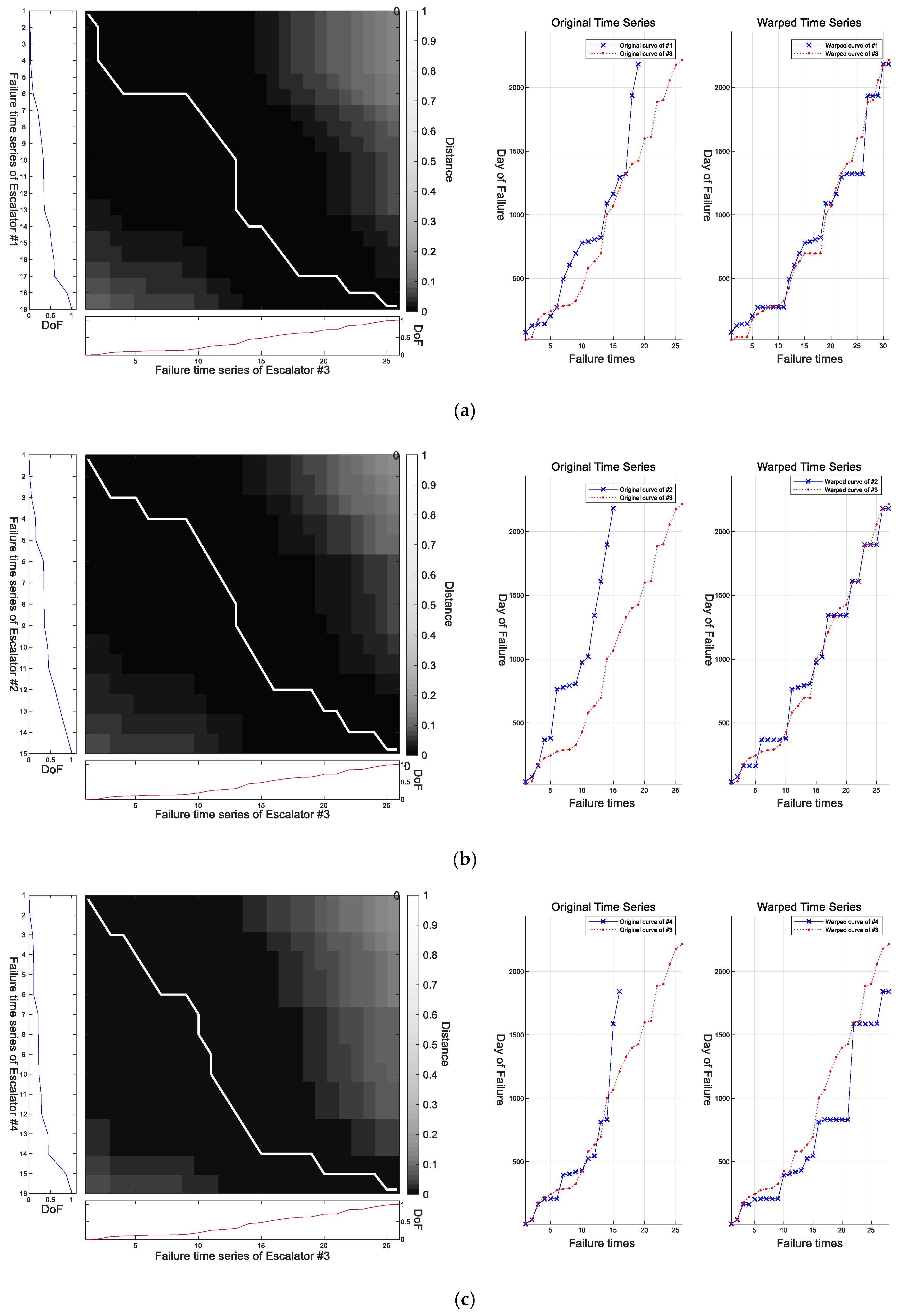
According to the comprehensive judgment from stationarity and complexity, the non-stationarity and complexity of escalator #3 is the smallest. The CSI of Escalator #3 is almost fifty times smaller than those of the others. In order to achieve the purpose of accurate prediction, it is necessary to reduce the influence of the other data disturbances during data modeling. The over-sampling characteristics of DTW can increase the number of time series while weakening the disturbances. Thus, DTW is used to warp other failure time curves with the data of the third escalator as a reference. The specific warping path and warped time series can be found in
Figure 10.
The white lines in the left of
Figure 10 are the warping path and the grayscale maps show the warping distance between the two time series. Figures on the right show the original time series and warped time series. It is easy to see that the new data after DTW have the same physical meaning as original data for the special warping path. Here, a specific analysis of the warped failure time series of Escalator #1 is given. As can be seen from
Figure 10, whether it is the red reference sequence #3 or the blue warped sequence #1, no new failure time is generated on the
y-axis, but only extended on the
x-axis, where the
x-axis represents the order or number of failures. Although some new samples were increased on the
x-axis, the occurrence time of failure is the same as before. It can still be regarded as the same failure. This is unambiguous in objective meaning. Meanwhile, it can be seen that due to the oversampling characteristics of DTW, the length of the time series after being warped has been increased. Although the increased samples do not affect the physical meaning of the failure time series, it is possible to increase training samples and increase the network’s understanding of the failure time series, which can further improve the training effect and prediction effect of the network.
In order to show the function of DTW, above-mentioned stationary indicators and complexity indicators are calculated after DTW with escalator #3 as referenced.
Table 2 shows the result after DTW pre-processing.
As shown in
Table 2 and
Table 3, the CSI is reduced to below 0.1 after DTW with the failure time series as the referenced sequence. A specific comparison of CSI before and after DTW preprocessing is summarized in
Figure 9 for a clear description. As shown in
Figure 11, the CSI of the other five escalators are reduced after DTW preprocessing with Escalator #3 referenced. They become more stationary and lower-complexity after matching with the failure time series of Escalator #3.
Besides, for the convenience of engineering applications, six sigma was applied to the analysis of the CSI of the failure time series after DTW to try to give a possible threshold of the CSI. In addition, the threshold can be used to distinguish whether the data sequences need to be warped before data modeling. The distribution interval of CSI can be given by , where is the mean value of CSI and is the variance. For above-mentioned data sequences after DTW, . Thus, the CSI value can be considered in the interval [0.0012 0.0396], and the upper limit of the interval is used as the judgment threshold considering the fault tolerance. That is, . For data sequences in this paper, if the CSI is less than CSIthreshold, DTW preprocessing is unnecessary before data modeling, otherwise, it is recommended to be warped with a sequence with a CSI less than CSIthreshold.
3.3. Results of LSTM and DCLNN
It is easy to see that no straightforward rules can be found directly from the failure time curve in
Figure 10. The LSTM is used directly to train and predict the data in
Figure 10. During the training process, the prediction goal is the failure time of the last day. Among them, about 90% of the time series data are used to train the LSTM NN, and the last 10% of the data are used to test the model and predict the failure time. The specific architecture and hyperparameters of CLNN can be found in
Figure 12. Tensorflow was used to build the above neural networks. A related repository was stored in the link (the same name with paper) on github.
Taking into account the time cost and prediction accuracy of network training, the recommended training epochs is around 200. Before data training and testing using a neural network, data normalization using Equation (18) is necessary.
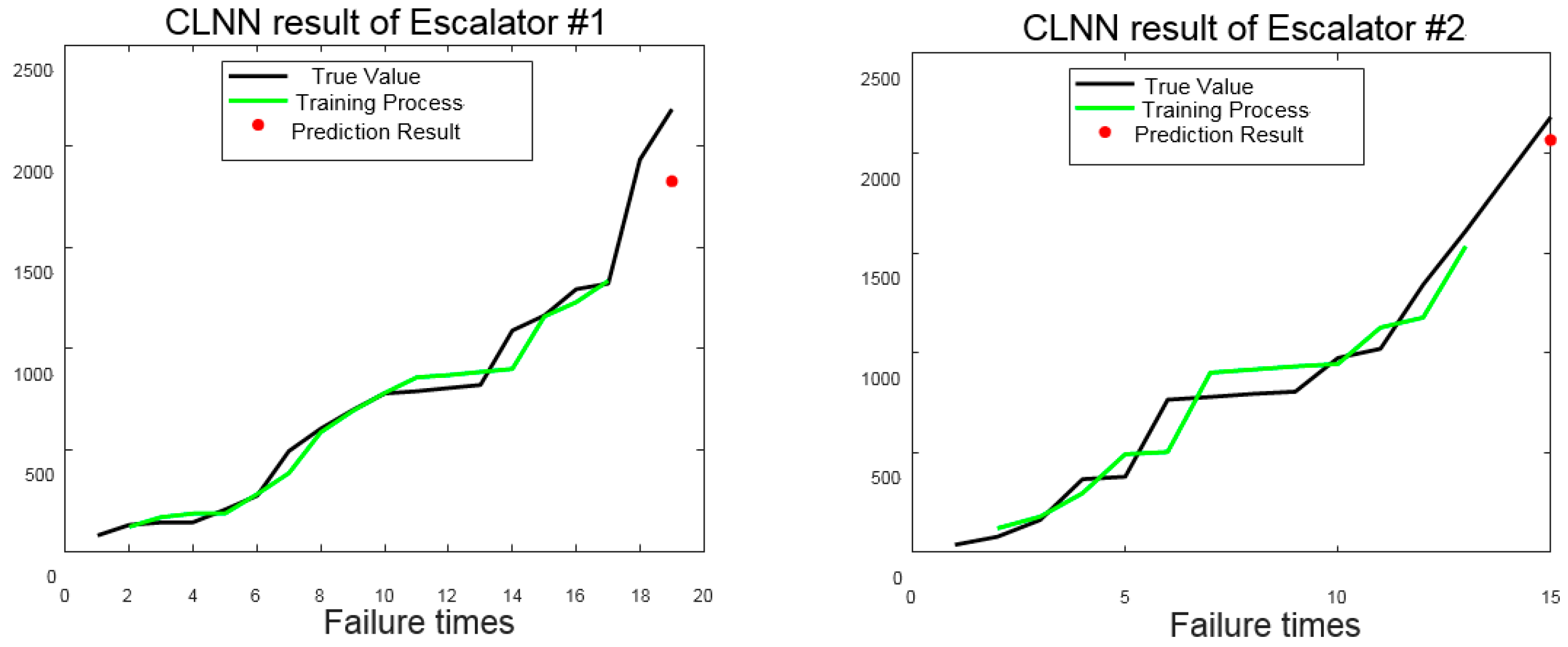
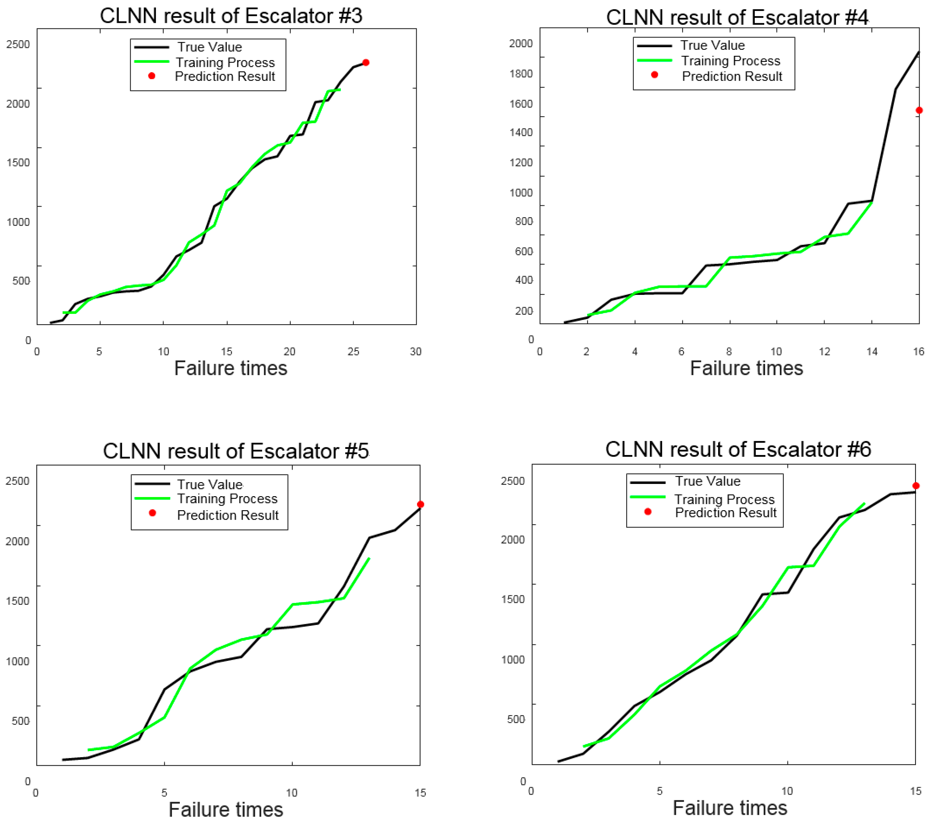
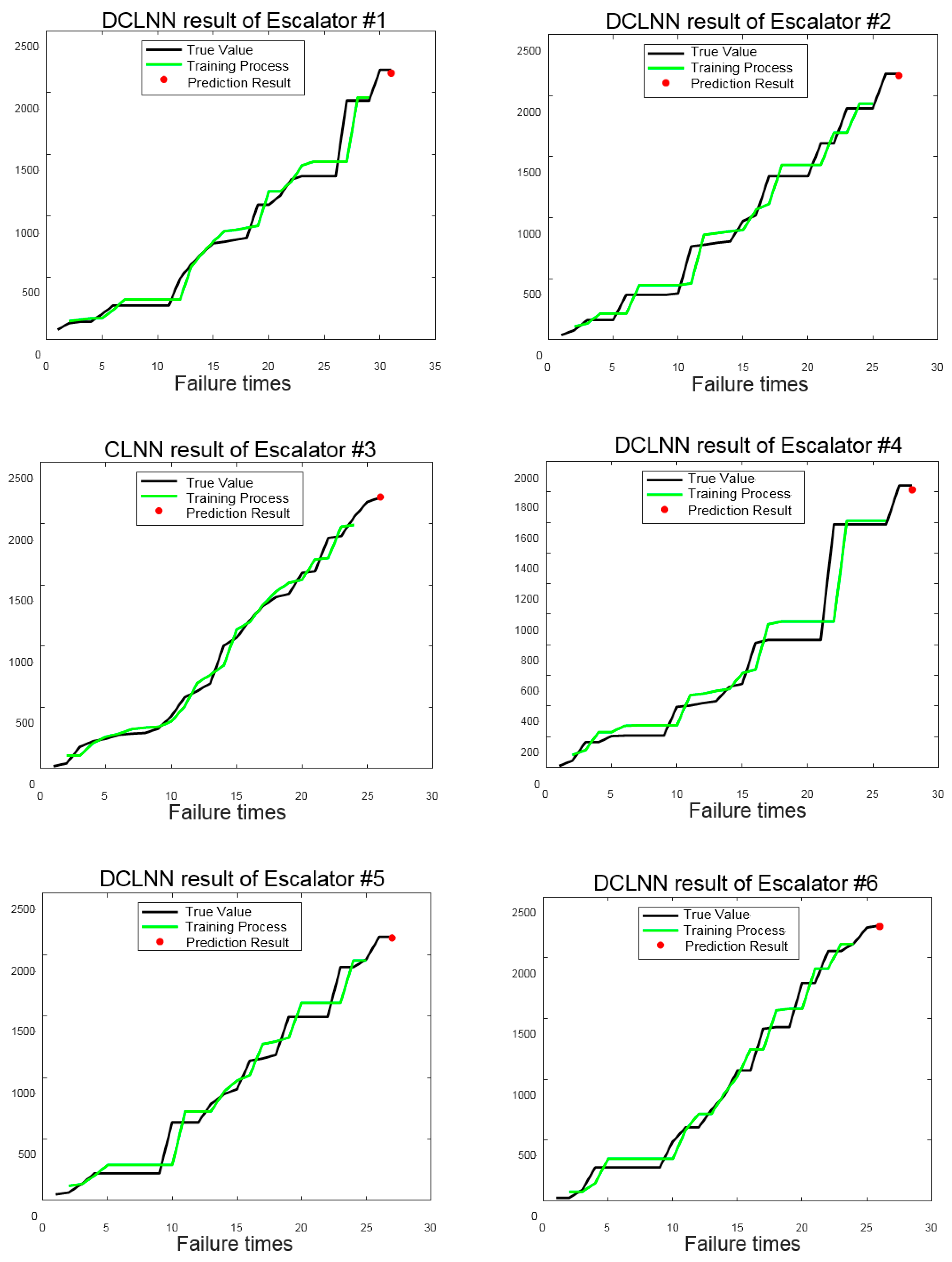
Then, the original failure time series of six escalators are first trained by the CLNN. The training process and prediction result are shown in
Figure 13. Training loss and testing loss are also given in
Figure 14.
Black lines are the true value of the failure time curve, green lines indicate the training process, and the red point shows the prediction result. All escalators except the third one have poor predictions that can be seen from
Figure 13 directly. The results are consistent with the result of CSI. The reason for the poor prediction of other escalators are: 1) The length of the data sequence is short, and the number of data used for CLNN model training and testing are also small; 2) the trend of the third escalator is stable with no obvious disturbance, while there are more or less disturbances in the time series data of the other five escalators. In addition, those disturbances make a big difference on modeling accuracy of the CLNN. Then, DTW is used to warp other failure time curves with the data of the third escalator as a reference. Using new data for training and prediction of the DCLNN, the results are shown in
Figure 15. Training loss and testing loss are also given in
Figure 16.
The prediction accuracy after pre-processing is significantly improved compared to the direct use of the original data. Here, the root-mean-square error (RMSE) is chosen to assess the prediction accuracy of escalators. The RMSE can measure the difference between two time series. The mathematical formula is:
The comparison results are summarized in
Table 3 and
Table 4.
Table 3 shows the RMSE of the training process between the original data and warping data.
Table 4 shows the RMSE of the prediction process between the original data and warping data. Although the RMSE in the training process changes a little, the RMSE has been reduced a lot in the prediction process. After pre-processing by DTW, the accuracy of the DCLNN is improved.
With DCLNN, the RMSE of the escalator can be reduced by an average of 83.96%. From
Figure 15, the accuracy of the prediction result can be reduced from a few hundred days to less than one month, in order to compare the accuracy of the proposed DCLNN model for failure time prediction of escalators. For a better explanation about the effectiveness of the DCLNN, the other three classical time series prediction methods (Kalman Filter, Nonlinear Auto Regressive Neural Network, Elman RNN, LSTM) are applied for data analysis of the third escalator. The results of these methods are shown in
Figure 17. The results intuitively show huge errors from the true value compared to results from the DCLNN.
3.4. Function of DTW
The use of DTW to warping time series can improve the prediction accuracy and reduce the mean square error. If the prediction effect of two time series is poor when using the neural network for the first time, the result is not obviously improved after using DTW. However, the result will have a significant improvement after DTW preprocessing if one of the time series is relatively good for prediction.
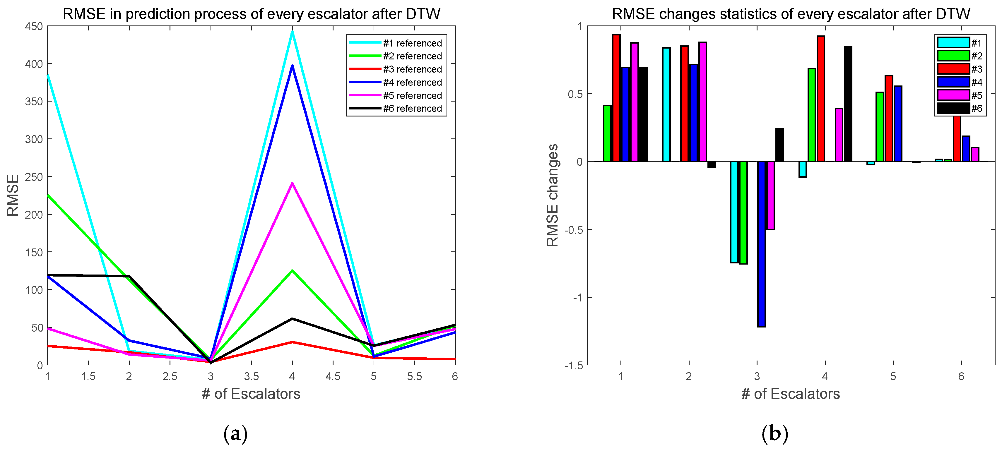
Table 5 concludes all RMSE values when using different time series as referenced data for DTW pre-processing and warping data for prediction using DCLNN.
Figure 18a is obtained from each column in
Table 5. It is clear to see that the MSE is smallest when choosing the third escalator as the reference time series in DTW preprocessing.
Figure 18b shows the RMSE improvement of DCLNN prediction after using different escalator data as the reference time series in DTW pre-processing. Similarly, the RMSE improvement of the third escalator is best compared to others. Meanwhile, the result in
Figure 18b shows that almost all MSE of the data sequences with different data sequences as referenced can be improved after DTW preprocessing. However, for the third escalator, the RMSE variation is negative. The main reason is that the data quality of the third escalator is best according to the CSI indicator. After DTW is preprocessed with other data as referenced data, the data quality is not as excellent as the third data itself. Therefore, for data with high quality, it is not recommended to use DTW for data preprocessing, otherwise it will reduce the data quality and increase the prediction error.
4. Conclusions
Failure time, as an important factor for the safe operation of escalators, is used for prediction by the proposed DCLNN neural network in this paper. Due to the short length of the failure time series, and the characteristics of random interference and non-uniform sampling, the failure time prediction is much more difficult. Naturally, higher data quality and a suitable neural network can help solve this problem. Considering the oversampling characteristics and similarity-matching performance of DTW, some inferior data with low stationarity and high complexity can be warped by referring to excellent data while retaining its original physical meaning. Such DTW-based data pre-processing can not only increase the sample numbers of short time series but also reduce the impact of disturbance data on the neural network. After data preprocessing, the combination of CNN and LSTM is used to train and predict the failure time series. With the help of CNN’s feature extraction ability, high-dimensional features can be trained to understand the failure time series more comprehensively. Then, these high-dimensional features can be used for time series prediction in LSTM. Based on the advantages of DTW, CNN, and LSTM, a strategy to combine data quality enhancement with deep neural networks is proposed to achieve the goal of failure time prediction for an escalator. Failure-recall data of an escalator are analyzed using the proposed DCLNN method, and the result shows that the proposed method can effectively reduce the root-mean-square error between the predicted value and the real value in the prediction process. At the same time, compared to some classical time series prediction methods such as the Kalman Filter, Nonlinear Auto Regressive Neural Network, and Elman RNN, the prediction accuracy of the proposed method is obviously improved. Besides, the function of the DTW was further analyzed to show that enhancing data quality can effectively improve the accuracy of prediction. The proposed DCLNN method can reduce the prediction time error of escalator failure to less than one month, which can provide scientific guidance for smarter maintenance planning and economic improvement.
However, due to the limited number of samples, the accuracy of the proposed method needs to be improved for better maintenance guiding, and a more reasonable threshold of CSI indicators needs further study before pre-processing in engineering application. Furthermore, the proposed method is currently applicable to the situation of two or more devices to improve the prediction accuracy. In the future, an in-depth study is necessary for the failure time series prediction problem of a single device under a small number of samples.


