Performance Assessment of a Renovated Precast Concrete Bridge Using Static and Dynamic Tests


Faculty of Civil Engineering, Slovak University of Technology, Radlinského 11, SK-810 05 Bratislava, Slovakia
*
Author to whom correspondence should be addressed.
Appl. Sci. 2020, 10(17), 5904; https://0-doi-org.brum.beds.ac.uk/10.3390/app10175904
Submission received: 12 July 2020
/
Revised: 20 August 2020
/
Accepted: 22 August 2020
/
Published: 26 August 2020
(This article belongs to the Special Issue Reliability Techniques in Industrial Design)
Abstract
:The article presents the development of a SHM (Structural Health Monitoring) strategy intended to confirm the improvement of the load-bearing capacity of a bridge over the Ružín Dam using static and dynamic load tests, as well as numerical simulations. The paper comprises measurements of the global response of the bridge to prepare a verified and validated FEM (Finite Element Method) model. A complex measuring system used for the tests consisted of two main parts: an interferometric IBIS-S (Image by Interferometric Survey-Structures) radar and a multichannel vibration and strain data logger. Next, structure–vehicle interactions were modelled, and non-linear numerical dynamic analyses were performed. As a result, the time histories of displacements of the structure from traffic effects were obtained. Their comparison with IBIS-S radar records proves that this method can be effectively used for assessing bridges subjected to common traffic loads. The results (measured accelerations) obtained by local tests in external pre-stressed cables are presented and a convenient method for acquiring the axial force in the cables is proposed.
1. Introduction
Bridges are among the most complex and important structures of civil infrastructure. They must operate in demanding environments, and withstand extreme loads and deterioration which occur during their operational lifespan [1]. Therefore, maintenance and monitoring of their state is crucial, mainly for safety and economic reasons [2]. Visual inspection represents a standard process in many countries [3]. As mentioned in [4], the identification of damages from visual inspections are usually influenced by the subjectivity of the expert. There are other issues with visual inspections—some locations are not accessible; at other times it is difficult to determine the severity of damage. Due to these reasons and possible road closures, bridge owners and managers are interested in automation of the process by using sensors. Many researchers across the United States [1], Europe [2,5,6,7,8], and Asia [9,10,11,12] have taken advantage of the rapid evolution of sensing technologies in the last few decades and implemented methods of structural health monitoring (SHM) to track the structural integrity of bridges. An important part of SHM is testing. Two main approaches to testing are known: destructive and non-destructive. Destructive methods use demolition of material to determine material characteristics. On the other hand, the advantage of non-destructive testing is that the observed structure will remain undamaged after a test. Therefore, non-destructive testing is a well-developed research and practical field, and vibration-based methods are one part of that field. According to [13], vibration-based SHM techniques can be divided into global non-destructive techniques, local non-destructive techniques, and long-term application of SHM techniques. Local techniques deal with one structural element, such as cables [12]. On the other hand, global techniques use data from a whole structure.
Furthermore, the testing methods can be divided according to how the response is excited: statically or dynamically. The design of static tests is less difficult, as only a stationary load is used. The possibility of easier evaluation is also advantageous, and the results can be simpler compared to the results from numerical models. On the other hand, they have less practical value, and they do not show the real behavior of structures during dynamic loads. Dynamic test methods that examine the behavior of structures under dynamic loads are mainly applied to bridges. These structures are loaded by moving vehicles, pedestrians, or ambient dynamic loads. The fast evolution of sensing technology has enabled the incorporation of SHM methods into the life cycle of bridges [14]. It must be noted that a visual inspection cannot be completely substituted by SHM methods. Several types of measuring devices and compatible sensors are now available. The most common types of sensors are strain gauges, accelerometers, speedometer gauges, temperature sensors, and optical sensors, among others. The above-mentioned authors mainly used one type of sensor in their studies. Strains were measured in [1], accelerometers were used in [5] and [8], and radar was applied in [9]. The combination of multiple sensor types was presented in [11]. A similar approach was selected in this work; a measuring device with the ability to measure accelerations, temperatures and strains was used in combination with the use of radar interferometry and a video camera.
This paper presents the development of a SHM strategy as an application of a fusion of well-known methods during various stages of testing (e.g., numerical modal analysis to obtain initial dynamic parameters, operational modal analysis [15], verification and validation of a FEM model [16], and vehicle–bridge interactions [17]) in order to obtain the global static and dynamic response of a reinforced concrete bridge, along with local measurements of strains in external cables. To obtain a verified and validated FEM model, various tests were performed (e.g., a static test (measurements of displacements and strains), a dynamic test (measurements of displacements and accelerations), and operational modal analysis). The verified FEM model can serve as a tool for evaluating various damage scenarios and predicting changes in bridge responses in these scenarios on the basis of future measurements.
This paper consists of multiple sections. Section 2 describes the bridge; Section 3 deals with the FEM model of the bridge and moving vehicles; Section 4 presents the measurement setup used for the tests; Section 5 is devoted to the verification and validation of the FEM model, with the results from the static test and operational modal analysis also presented here; Section 6 contains the comparison of the time history analysis performed by a numerical calculation and the measured displacement in the middle of the main span; Section 7 shows the results of a local non-destructive test of external pre-stressed cables and finally, the main conclusions are presented in Section 8.
2. Bridge Description
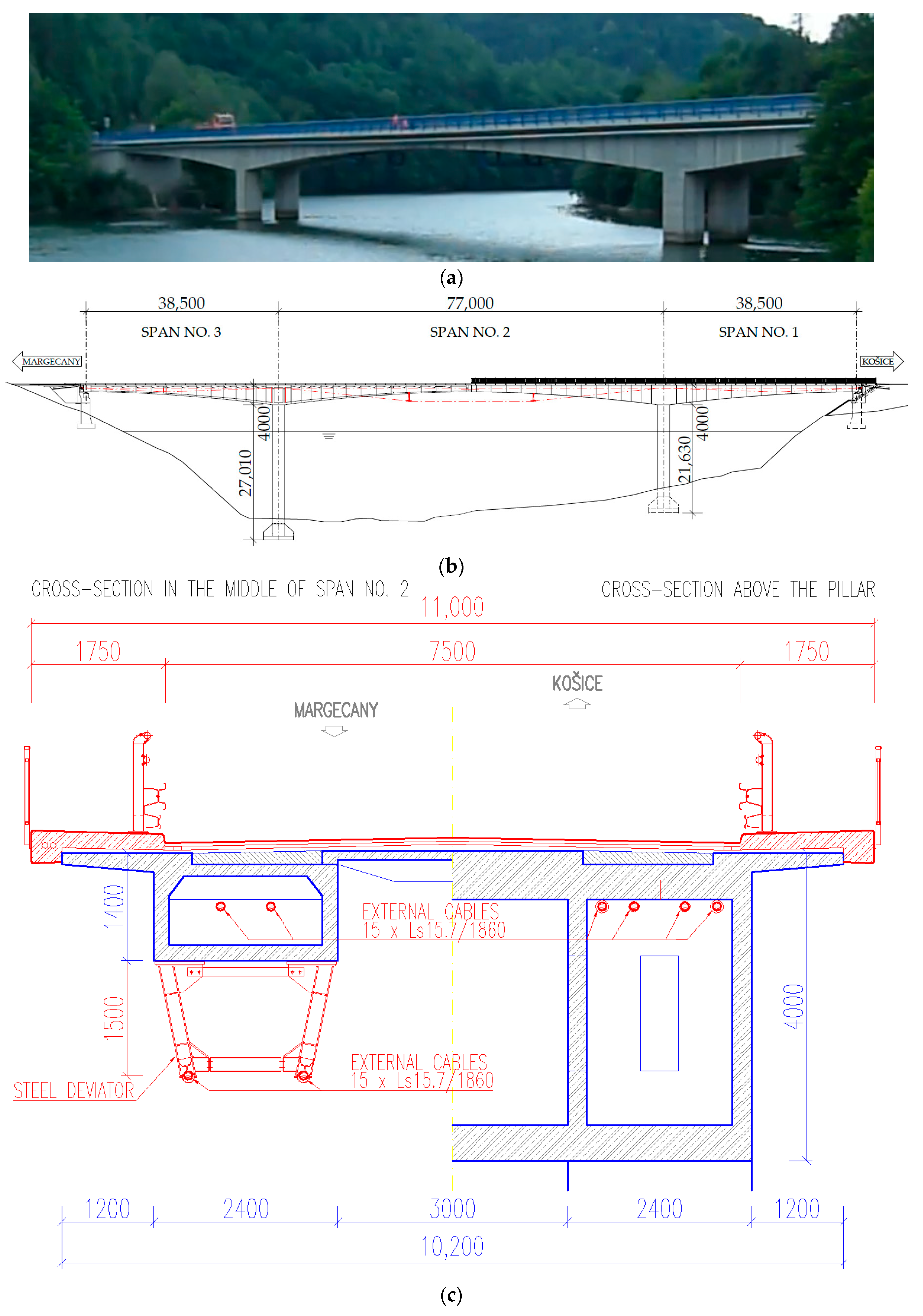
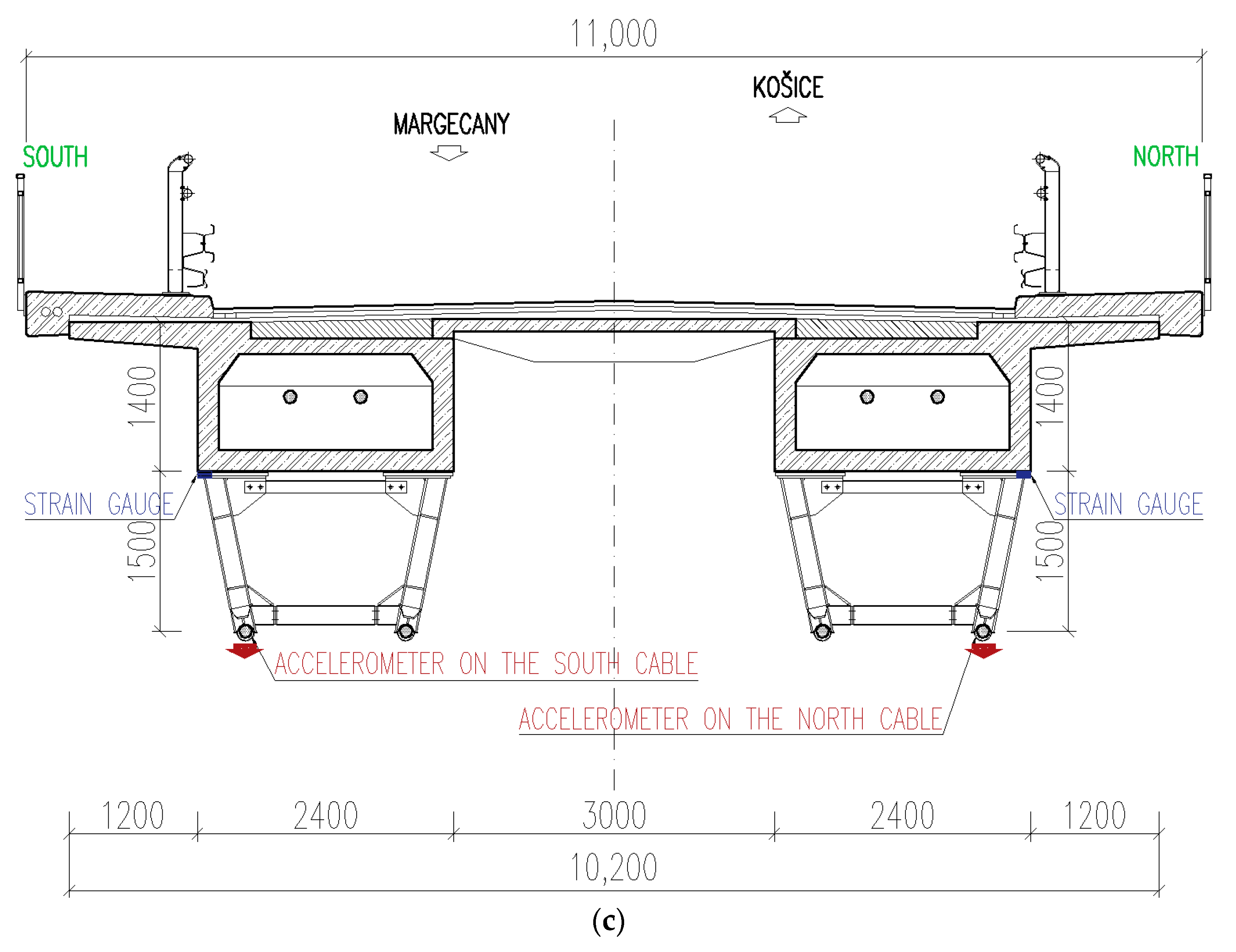
The bridge over the Ružín Dam has been in operation since 1967 and was renovated in 2017 (Figure 1) as a result of its full closure in 2016 due to its critical state. The reason for the closure and for the necessity to renovate was the permanent (visible) displacement in the middle of the main span. The bridge structure consists of two parallel tapered box-girders with various heights between 1.4 m and 4.0 m. Pre-cast slabs are embedded between the two box-girders. The width of the bridge comprises the road surface (7.5 m) and the walkways on both sides (1.75 m); overall, the bridge is 11.0 m wide. The total length of the bridge is 154.0 m.
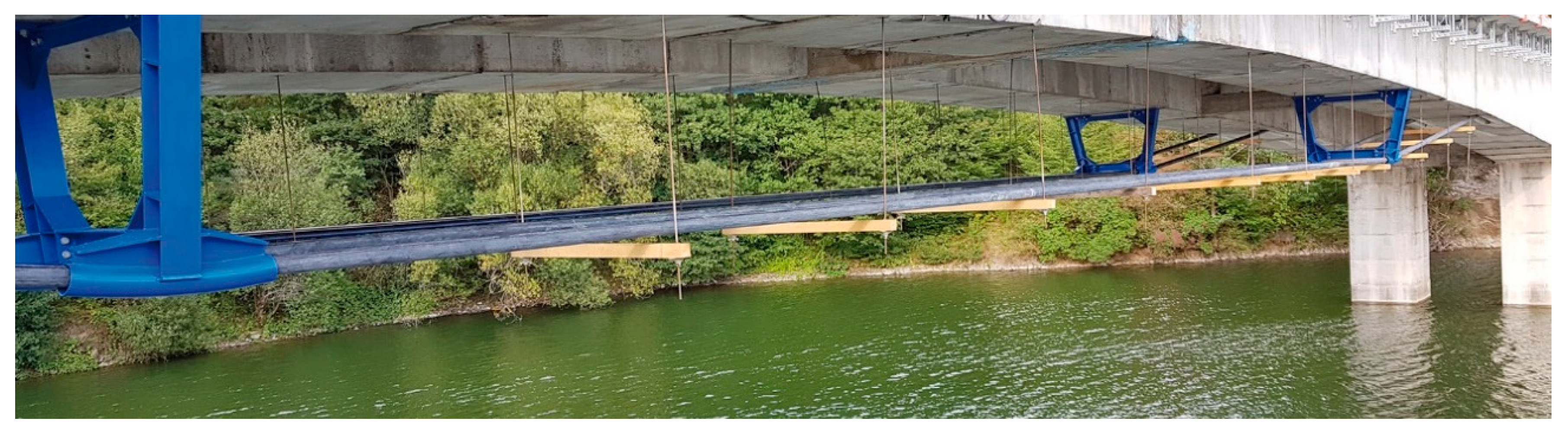
The bridge was repaired by changing the original structural system. The reconstruction was carried out by reinforcement of the original joint in the middle of span no. 2 and by the addition of external pre-stressed cables (Figure 2). Pre-stressed cables consist of two groups. The first group of cables passes over the outer side of the box-girders and is fixed by additionally mounted steel deviators (two cables per box-girder). The second group of cables is placed inside the box-girders (two cables per box-girder). Therefore, the overall strengthening consists of eight cables (15 × LS15.7/1860; for geometric and material characteristics, see Table 1 and Table 2).
The pillars with heights of 29 m and 24 m are monolithically connected to the load-bearing structure. A new sloping abutment with an approach slab was built in 2017. Renovation of the wing walls was realized by coupling reinforced concrete walls. Concrete C30/37 and steel B500 (B) were used.
The bridge is of great importance in the regional road network. According to Slovak Road Administration data [19], in 2015, more than 3300 vehicles passed over the bridge daily. Therefore, bridge closure could cause significant complications since alternative routes are more than 30 km longer.
3. Numerical Modelling of Vehicle–Bridge Interactions
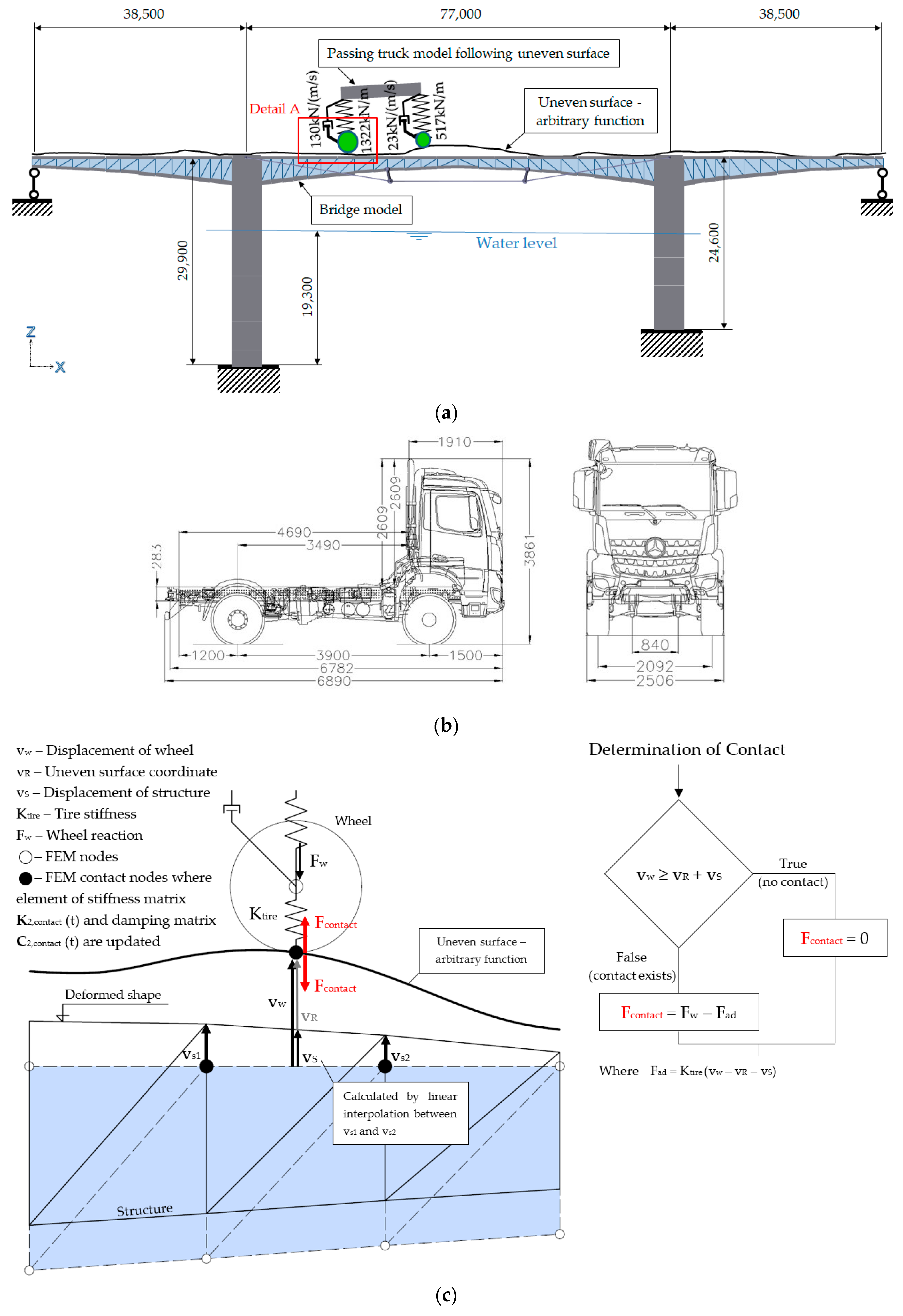
The 2D FEM model of the bridge and a passing truck were prepared (Figure 3) and numerical analyses were performed before executing the in situ tests in order to achieve the expected displacement of the bridge. The slab of box-girders was modelled with SHELL elements with a constant thickness of 0.2 m (width); flanges were modelled with BEAM elements: the upper flange had a constant height of cross section of 0.254 m, the bottom flanges had an increasing height of cross section, starting from 0.253 m in the middle of the span to 0.47 m in vicinity of the pier. The characteristics of cables are listed in Table 2. All concrete elements were modelled with Young’s modulus of elasticity E = 36 GPa. Pillars were modelled with beam elements with cross sections of 2.4 × 2.4 m. Fixed supports were assumed for both pillars, with joint supports at the beginning of the first span and the end of the last span.
The added cables (characteristics in accordance with Table 1 and Table 2) were considered TRUSS elements. MASS elements represent the extra weight of accessories. The contribution of the water mass on immersed piers was also added according to [20] with a value of 6800 kg/m.
3.1. Testing Vehicles
Mercedes Benz 1836 AK trucks were utilized for static and dynamic tests of the bridge. Their characteristics were assumed according to technical documentation (weighing ticket issued by a certified laboratory before the tests) and are listed in Table 3. The characteristics of the axles for Truck 1 are listed in Table 4. Truck 1 was only used for the dynamic test, whereas both trucks were used for static tests.
3.2. Non-Linear Dynamic Analysis of the Vehicle–Bridge Interaction
The FEM model including both the structure and the vehicle was used for the evaluation of the dynamic tests. The code was prepared in such a way that it is possible to define the arbitrary function of an uneven surface (Figure 3a), which characterizes the displacement differences between truck contact DOFs (Degree of Freedom) and structure DOFs at particular time instances. These differences cause vertical inertial forces arising between the truck and the structure, and therefore result in additional dynamic load of the bridge. It is also possible to control the loss of contact. For the tested bridge, a new roadway was recently constructed, so only an arbitrary obstacle was assumed as an uneven surface. The tests included truck passage over the bridge at different velocities while crossing the uneven surface created by an artificial obstacle in the middle of span no. 2. The measurements were carried out during light traffic, so a particular case when only the testing truck was present on the bridge was analyzed. However, the dynamic response can also be analyzed assuming a complete traffic flow by recording all passing vehicles. The advantage of this method is that there is no need for significant traffic restrictions, which is the most convenient way of performing tests for bridge authorities.
To calculate the dynamic response of the structure, a non-linear numerical analysis assuming a vehicle–bridge interaction was performed. Contact effects depend on the velocity of the vehicle and on the uneven surface function between the bridge deck and the axle. Thus, the overall response of the vehicle–bridge system is calculated according to the system of equations in every time step:
where M is a mass matrix, C(t) is a damping matrix, K(t) is a stiffness matrix, f(t) is a vector of external loads and y(t) is a vector of displacement.
Special attention is paid to vector elements with “contact” indices where the values do not depend only on TH (Time History) analysis, but also on the uneven surface. Loss of contact, which can occur in cases of higher speed, is also incorporated into the analysis. The procedure by which contact force and contact loss were analyzed is described in Figure 3c, where displacements of the wheel vw have been compared with the sum of displacements of the structure vs and the uneven surface coordinate vR defined in a particular time step. If the difference between the wheel and the structure ∆structure − wheel = vw − vs − vR is greater than zero, then loss of contact is expected and the zero-contact force Fcontact acting between the vehicle and structure is assumed. Otherwise, contact still exists and the value of the contact force is calculated as the wheel reaction, depicted as Fw, acting on the axle and additional force, Fadd, satisfying the correct condition of continuity of displacements; i.e., wheel is located on the structure (also assuming uneven surface). The value of Fadd is a product of tire stiffness Ktire and ∆structure − wheel.
4. Measurement System
4.1. Accelerometers and Strain Gauges
A complex measurement system (able to measure accelerations, strains, and temperatures simultaneously by up to four devices) using National Instruments equipment was used. It was developed by one of the authors in collaboration with mechanical engineers [21]. It consisted of two devices for this procedure: NI cRIO (National Instruments Compact Reconfigurable Input Output) 9067 with four NI 9234 modules, and NI cRIO 9074 with two NI 9234 modules. The NI 9234 input module is an analogue-to-digital converter capable of measuring acceleration. The number of modules used allowed us to measure 24 channels. There was also one NI 9237 input module for the measurement of strain gauges. Temperature measurements formed an important part of the test. One NI 9211 input module allowed for measuring air temperature, as well as the structure temperature, using contact temperature sensors. Four temperature sensors, two strain gauges and 24 accelerometers were used simultaneously.
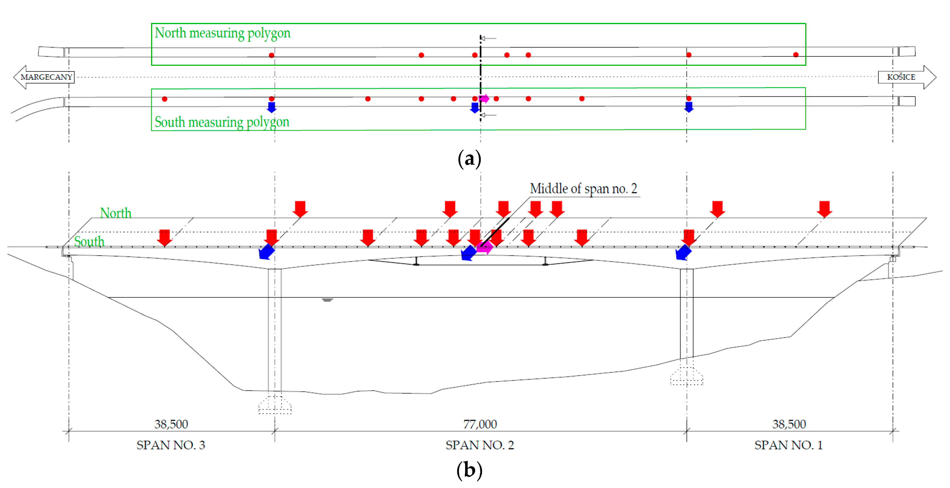
Accelerations in the Z-direction (vertical) were measured with 18 sensors (labelled with a red arrow); accelerations in the Y-direction (lateral) were measured with three sensors (labelled with a blue arrow, and accelerations in the X-direction (longitudinal) were measured with one sensor (labelled with a purple arrow). Two accelerometers were mounted by a magnetic pad on the external pre-stressed cables approximately in the middle of span no. 2 (Figure 4). Two measuring polygons using two measuring devices with separately connected accelerometers were placed along the footpaths to obtain the torsional mode shapes. The first polygon with eight accelerometers was on the north side, the second one with 16 accelerometers was on the south side. The synchronization of measuring devices was carried out via an FTP (file transfer protocol) using an FTP cable placed under the bridge girder to be protected from traffic. This arrangement of the devices reduces the measurement preparation time, as the necessary cable lengths were shortened.
Accelerometers (PCB—PicoCoulomB—Piezotronics 393B31) in combination with the NI 9234 input modules, measured frequency higher than 0.5 Hz with an interval of amplitudes ±4.9 m/s2. The resonant frequency of the sensors is over 0.4 kHz. The high sensitivity of these sensors makes them suitable for ambient vibration measurements. Accelerometers (MMF—Metra Mess—und Frequenztechnik—KS48C) were also applied with a higher range of amplitudes (± 58.9 m/s2) and the resonant frequency was above 7 kHz. Strain measurements were performed using HBM (Hottinger Baldwin Messtechnik) 50/120 LY41 strain gauge sensors (in the “Half Bridge” set up, i.e., one strain gauge is measuring the structure and one strain gauge is a dummy), suitable for concrete structures. Sensor resistance was 120 Ω, and strain factor was 2.09. K-type thermocouple contact sensors (SENSIT type TCS190) were used for the measurement of the structure temperature. Air temperature was measured by the SENSIT type TG4 thermocouple. Both air and structure temperatures were measured during the test (Table 5).
4.2. Interferometric Radar
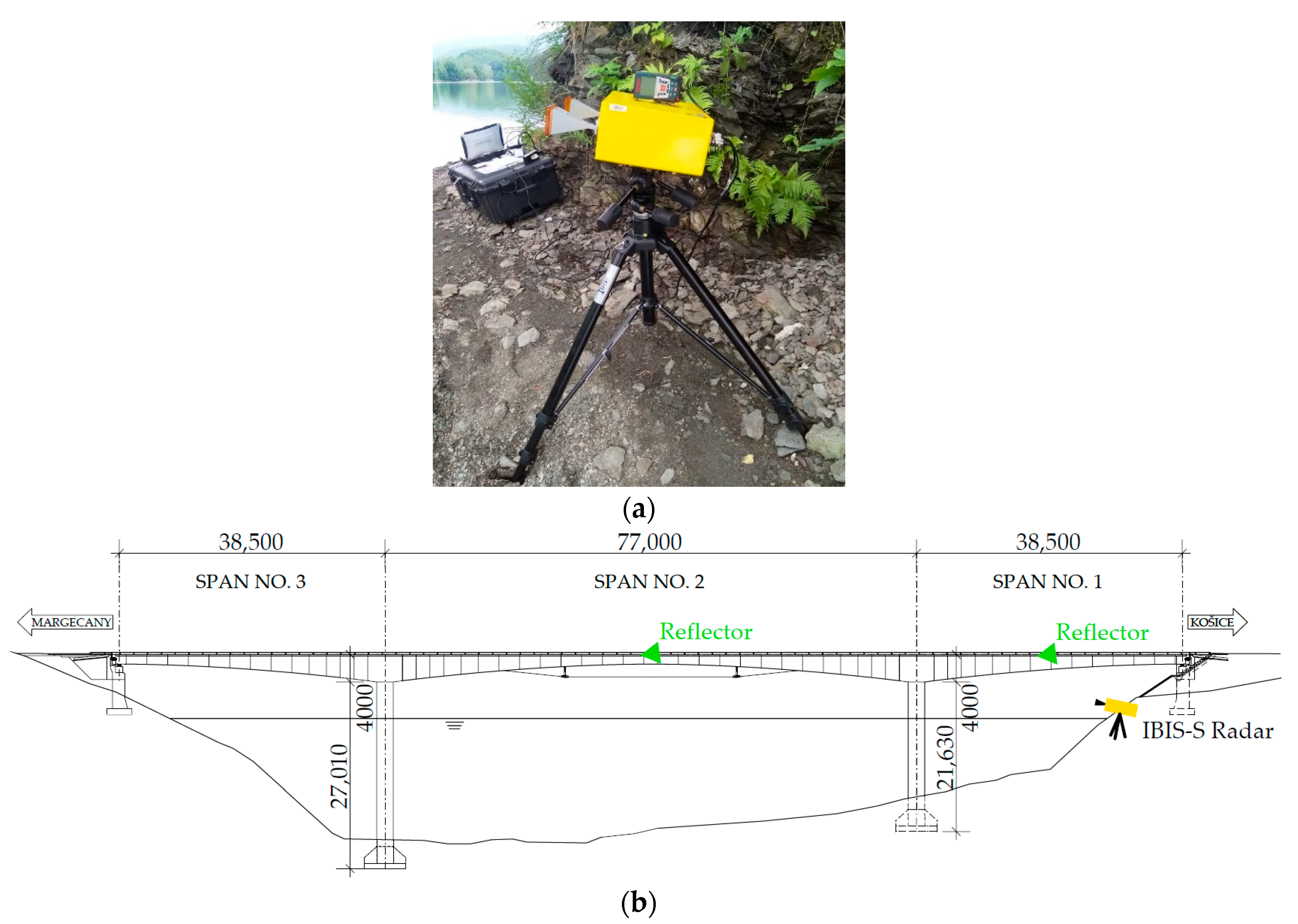
Dynamic displacement measurements were repeatedly performed using the IBIS-S interferometric radar with type 3 antennas from IDS (Ingegneria dei Sistemi) (Figure 5a). The radar was used for static and dynamic tests of the bridge.
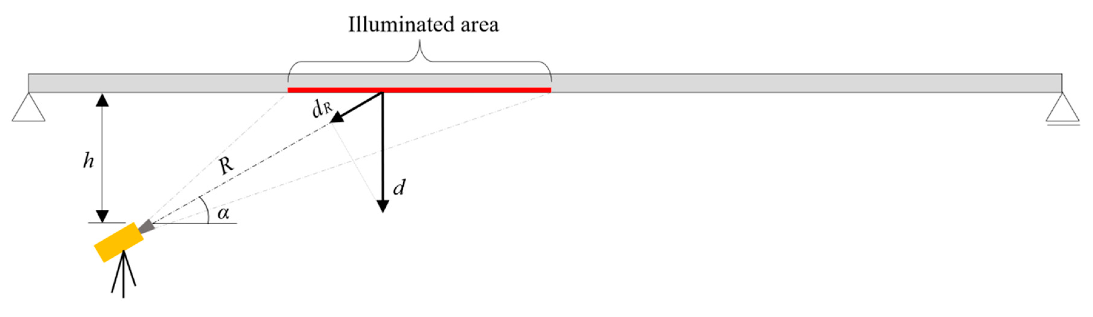
Interferometry is a radar technique that evaluates object displacement by comparing phase shifts of the electromagnetic waves reflected by the object in different moments in time [22,23]. The IBIS-S system simultaneously measures the radial displacement (dR)—the displacement in the direction connecting the device and the monitored point on the structure (Figure 6)—of all points of the area illuminated by the antenna beam.
Radial displacement dR must be projected in the direction of effective displacement d (in the vertical direction) (Figure 6).
It is important to identify the measured point on the structure as accurately as possible. For this reason, two reflectors (Figure 5b) were used and mounted at the locations where significant displacements were expected. It is necessary to know the radial distance R and the corresponding vertical distance h from the radar (Figure 6).
The measurement is extremely fast and relatively accurate. The accuracy of the measurement depends on the ratio of the signal to the noise of the point under consideration. Thus, it depends on the environmental effects (which can be eliminated) and on the distance from the measured point. The greater the distance, the lower the intensity of the reflected signal. Displacement measuring accuracy depends on the intensity of the reflected signal. The accuracy of the IBIS-S system is up to 0.1 mm as declared by the manufacturer. By installing artificial reflectors in specific points, the reflectivity of the target was improved. The radar was placed on the bank of the dam under span no. 1 (Figure 5b). Each measurement was performed in dynamic mode with a sampling rate of 200 Hz.
4.3. Measurement Stages
All of the above-mentioned measuring equipment was synchronized during the following stages of the measurements:
- Static tests (displacements, strains) during light traffic.
- Dynamic tests (weighed truck was passing over the uneven surface).
- Vibration measurements during full operation (results of operational modal analysis).
The traffic during the entire procedure was not stopped continuously for a single day. The static and dynamic tests were carried out during light traffic with passing cars briefly delayed in front of the bridge (outside of morning and afternoon rush hours). During the static test, two vehicles were passing over the bridge at a maximum speed of up to 5 km/h; during the dynamic test, a single vehicle (Truck 1) was passing over the bridge at various speeds from 5 km/h to 60 km/h. During the dynamic tests, the traffic on the bridge was recorded using a video recorder in order to set the speed of passing vehicles for numerical calculations and to omit the data records with heavy trucks from operational modal analysis.
Besides these adjustments, the bridge had to be assessed under operational conditions. Ambient vibrations were also caused by the wind; its effects were measured by an anemometer, but during the measurement phase, there was small wind velocity (v < 0.5 m/s) recorded and the impact was negligible.
5. Comparisons of Calculation and Test Results to Verify and Validate the FEM Model
In order to verify and validate the FEM model according to [16], selected static and dynamic parameters were evaluated from measurements. The accelerations, displacements and strains were compared with numerical results to check the input values of the model and to improve its quality. Because of that, it can be used to make accurate predictions in the future. In this section, the in situ tests of selected parameters are presented, along with the results from the verified and validated FEM model.
5.1. Displacements
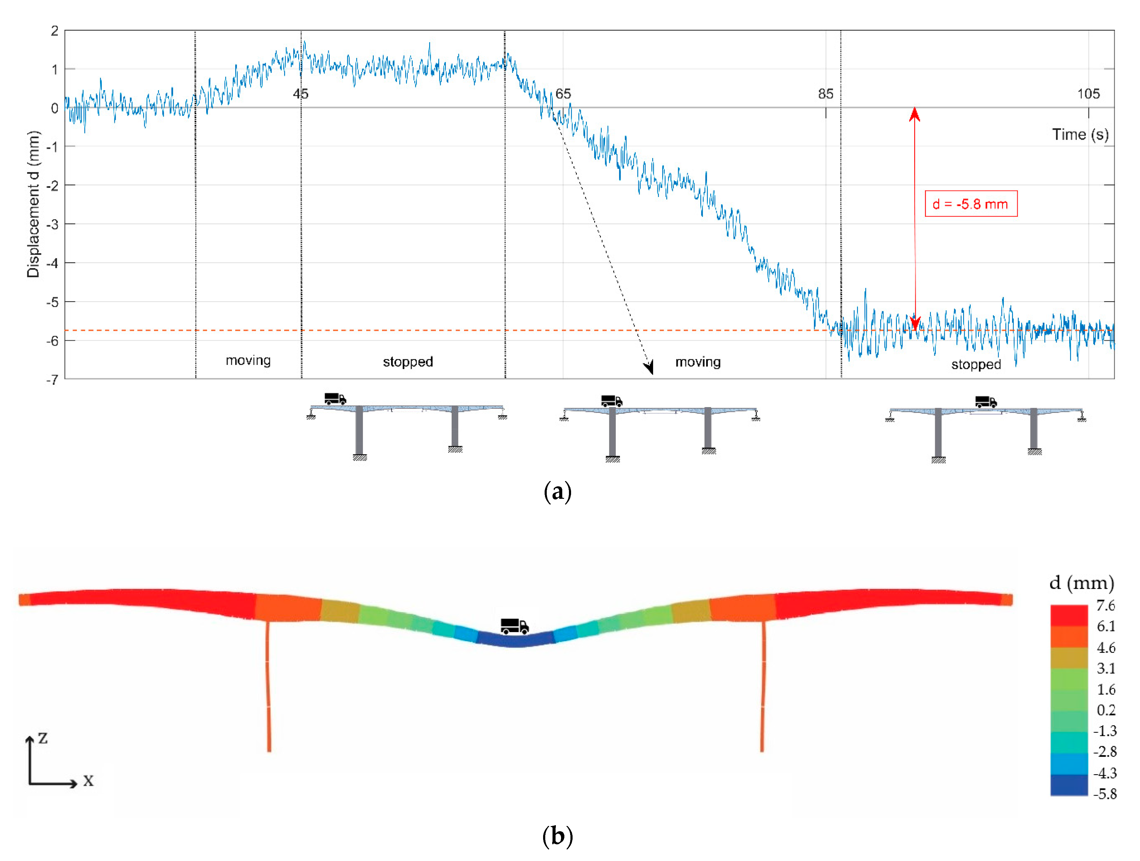
During a test of static displacement, two trucks were passing slowly (a maximum speed of up to 5 km/h) over the bridge and stopped briefly in the middle of span no. 2. A displacement time history was recorded by IBIS-S radar. Figure 7 shows good conformity between test and numerical analysis.
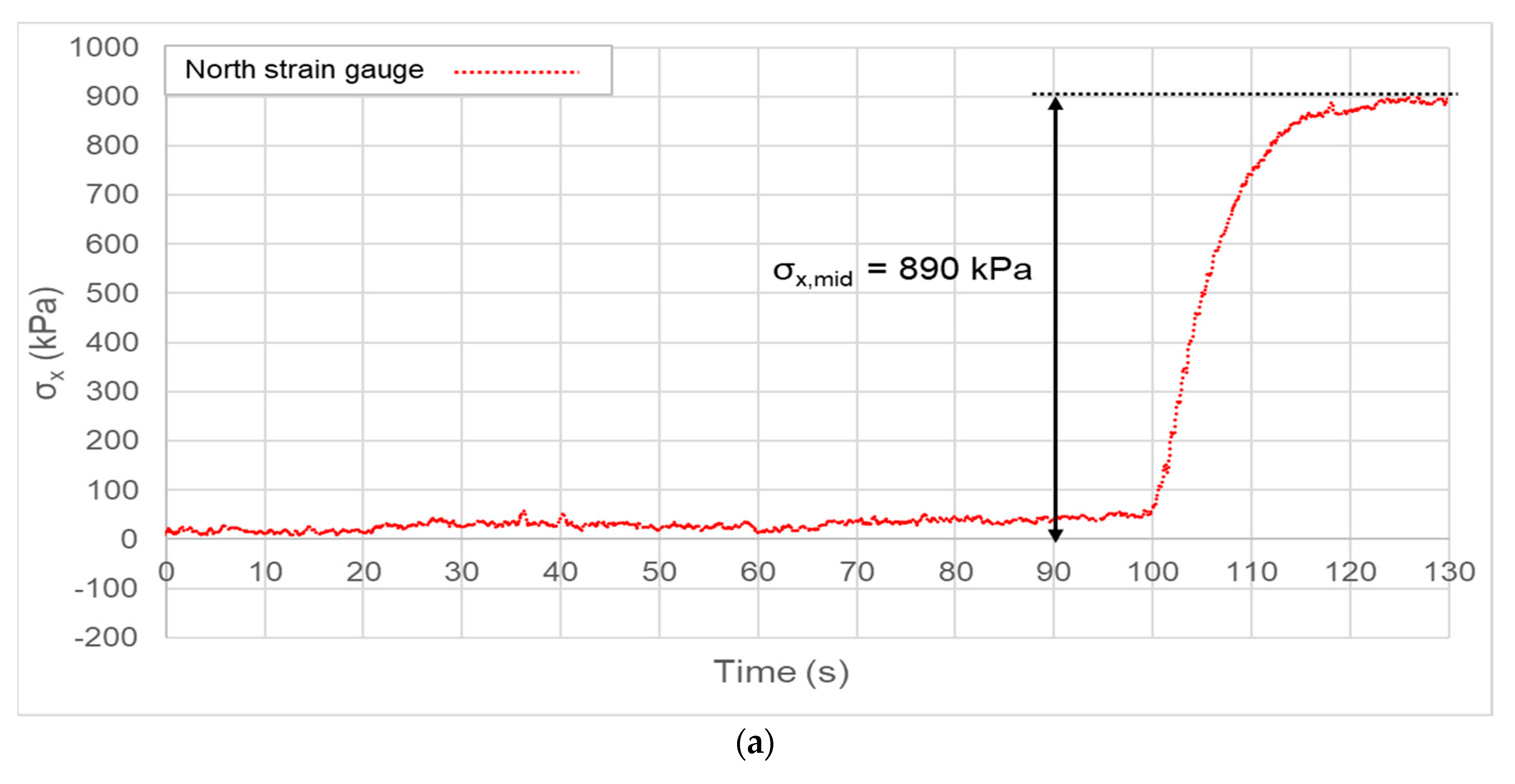
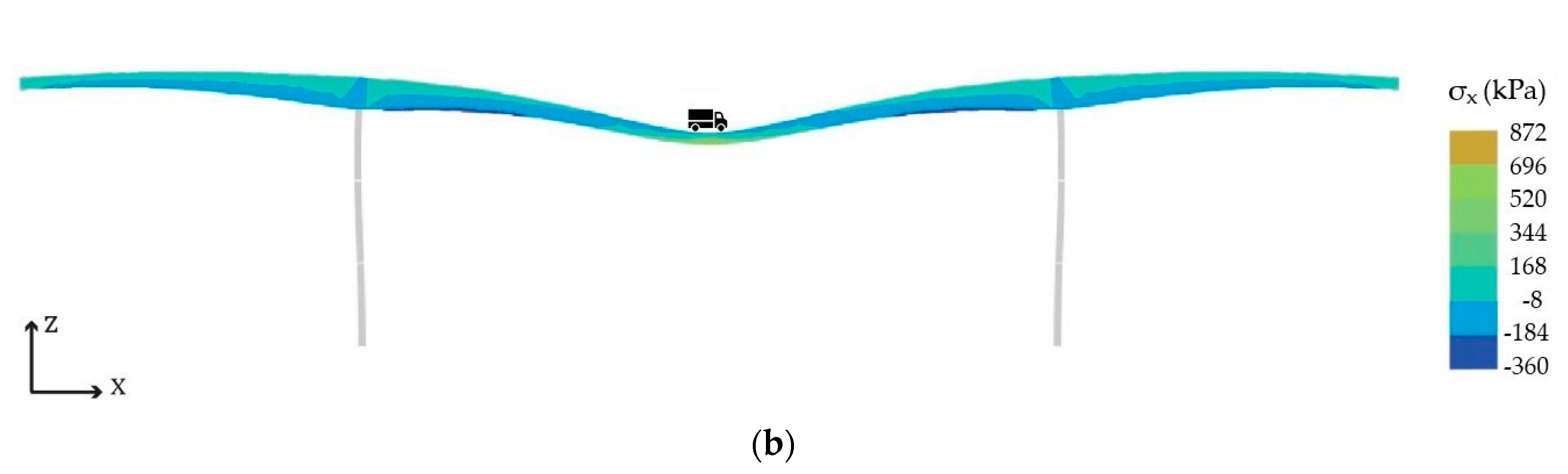
5.2. Strains
During a light traffic period (described in Section 4.3), two heavy trucks stopped in the middle of span no. 2. Figure 8 shows a comparison of stresses σx in the middle of span no. 2 (Figure 4) obtained by calculation from measured strains using strain gauges and E-modulus (Figure 8a), and numerical calculation from the presented FEM model (Figure 8b). It shows that the values correspond very well (measured value of 890 kPa vs. 872 kPa calculated by the FEM).
5.3. Natural Frequencies and Mode Shapes
An operational modal analysis (OMA) was performed on the bridge to obtain data for the validation of the FEM model [16]. Moreover, the aim of OMA was also to confirm that the global frequencies do not have a significant influence on the natural frequency of the free cables.
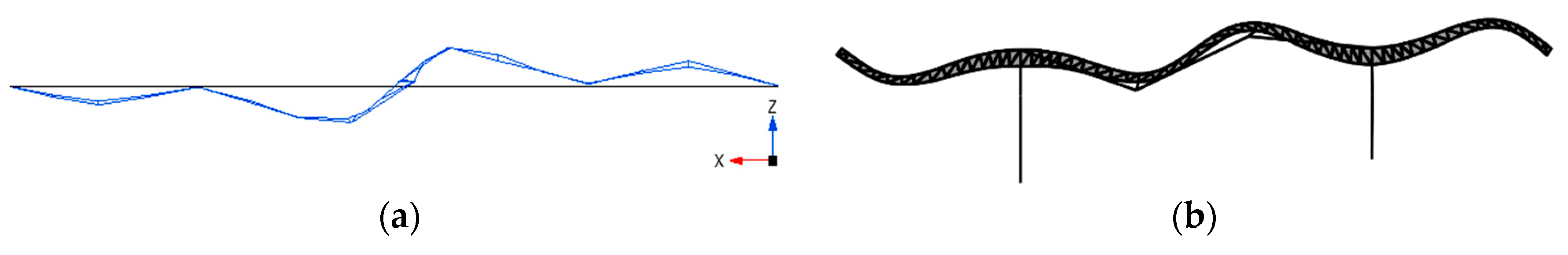
The data obtained from the NI 9234 modules (analog to digital converter (ADC)) were raw, without any physical unit. Because of that, the measured accelerations (sampled at 2 kHz) were pre-processed in the first step. The raw data were calibrated using the developed code and the data calibration list of each sensor. After this procedure, the time series had the appropriate unit of acceleration (m/s2). Then, the digital low pass filter with an eighth-order Chebyshev type I filter with a 15 Hz cut-off frequency was applied in both the forward and reverse direction in order to remove all phase distortions. Subsequently, records were down sampled to 50 samples/s. After that, each signal was high pass filtered with a fourth-order Butterworth filter with a 0.2 Hz cut-off frequency, again in both the forward and reverse direction, similarly to [24]. Finally, the pre-processed data were analyzed in the ModalVIEW software. The possibilities of the ModalVIEW software (stabilization charts) were used for extracting modal parameters such as natural frequency, damping ratio, and corresponding mode shape. Stabilization charts were calculated using the stochastic subspace identification (SSI) method, which is described in [25] in detail. These cut-off frequencies were set because the natural frequencies calculated by the initial FEM model fell within this interval. In this case, the stability criteria from the stabilization charts used were chosen similarly to [26], specifically: 1% for frequency stability, 5% for damping stability, and 2% for mode shape stability. System identification (SI) of the bridge was done in accordance with the mentioned criteria, and the obtained experimental results were compared with the FEM calculations (Figure 9, Figure 10, Figure 11 and Figure 12).
Table 6 shows the comparison of natural frequencies of the FEM model and the measurement. Since the FEM model is only 2D (coordinate system X axis vs. Z axis), natural frequencies and their corresponding mode shapes are only shown in Z directions. There is a good conformity between the measured and the calculated natural frequencies for the corresponding mode shapes.
Additionally, Cross-MAC (Modal Assurance Criterion) values, similar to [27] are presented. The formula is as follows:
where is the ith mode shape vector obtained by the FEM model, and is the jth mode shape vector of the measured structure as computed by the SSI method. If the value of Cross-MAC is nearing 1, the match between two mode shapes is complete. On the other hand, if the value of Cross-MAC is 0, then the mode shapes are entirely different. The gathered differences of the Cross-MAC values are smaller than 10%, which means that the mode shapes were identified correctly. Such a good conformity between the real response and the response from the prepared FEM model can be later used for SHM purposes, e.g., for the simulation of damages or a check of a suitable method of damage detection.
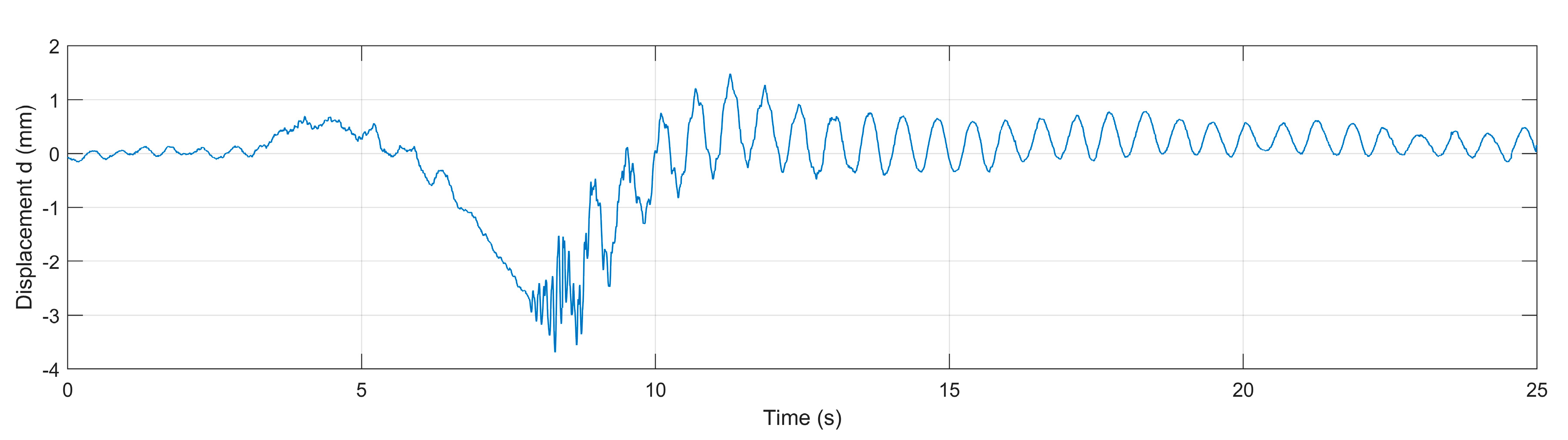
The result of the SSI method (the third natural frequency) was compared to the natural frequency obtained by the IBIS-S radar. As seen in Figure 13, the response of the structure after the truck left the bridge (at about 13 s) can be described as free damped vibration. Specifically, ten sine waves appeared between the times t1 = 13.72 s of the first peak and t2 = 19.56 s of the last peak. Thus, the third natural period Td of the structure can be calculated; the result is Td = 0.584 s. The third natural frequency related to vibration in the vertical (Z) direction is then equal to 1.71 Hz. The same result of the third natural frequency was obtained from measured accelerations (Table 6). The identified natural frequencies from two independent devices (complex measurement system vs. IBIS-S radar) confirmed the precision of the performed measurements. However, some mode shapes could not be extracted from the measured acceleration data because of the relatively small number of accelerometers used, especially in the lateral (Y) direction.
6. Evaluation of Dynamic Displacements of the Bridge
The dynamic tests with the truck passage at different velocities were performed to obtain the dynamic response of the structure. Only traffic load was assumed in the numerical calculations. The wind effects during the tests were negligible and therefore not incorporated into the calculations. Effects of the structural dead weight were not included in the presented displacements.
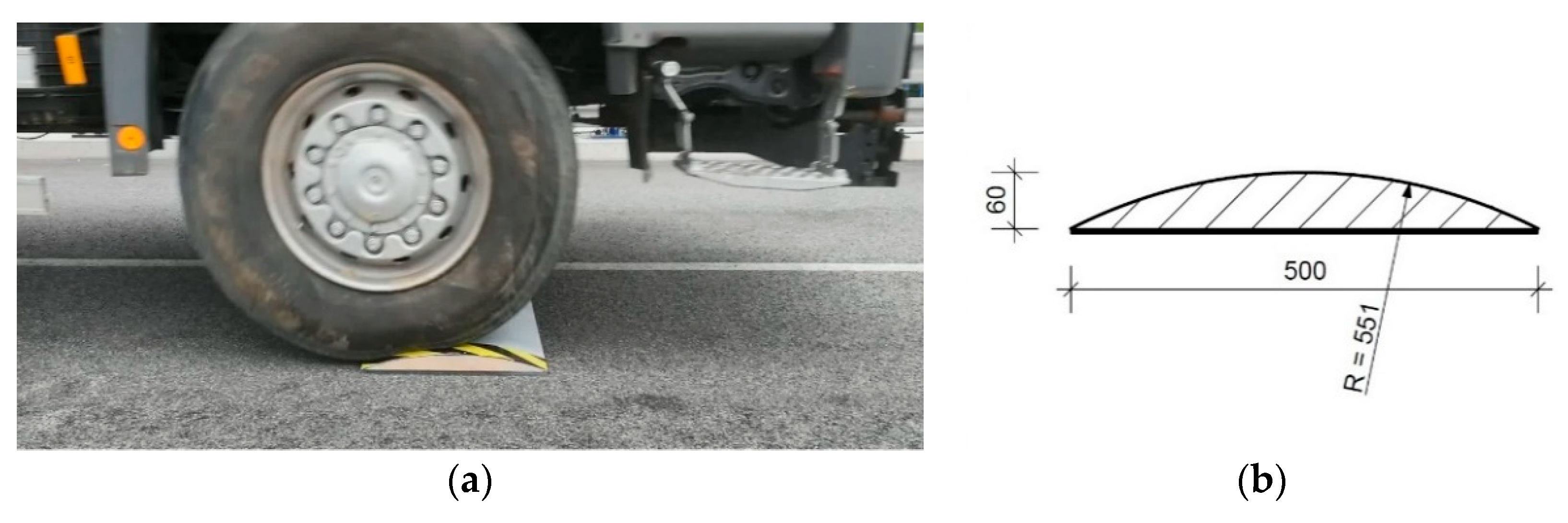
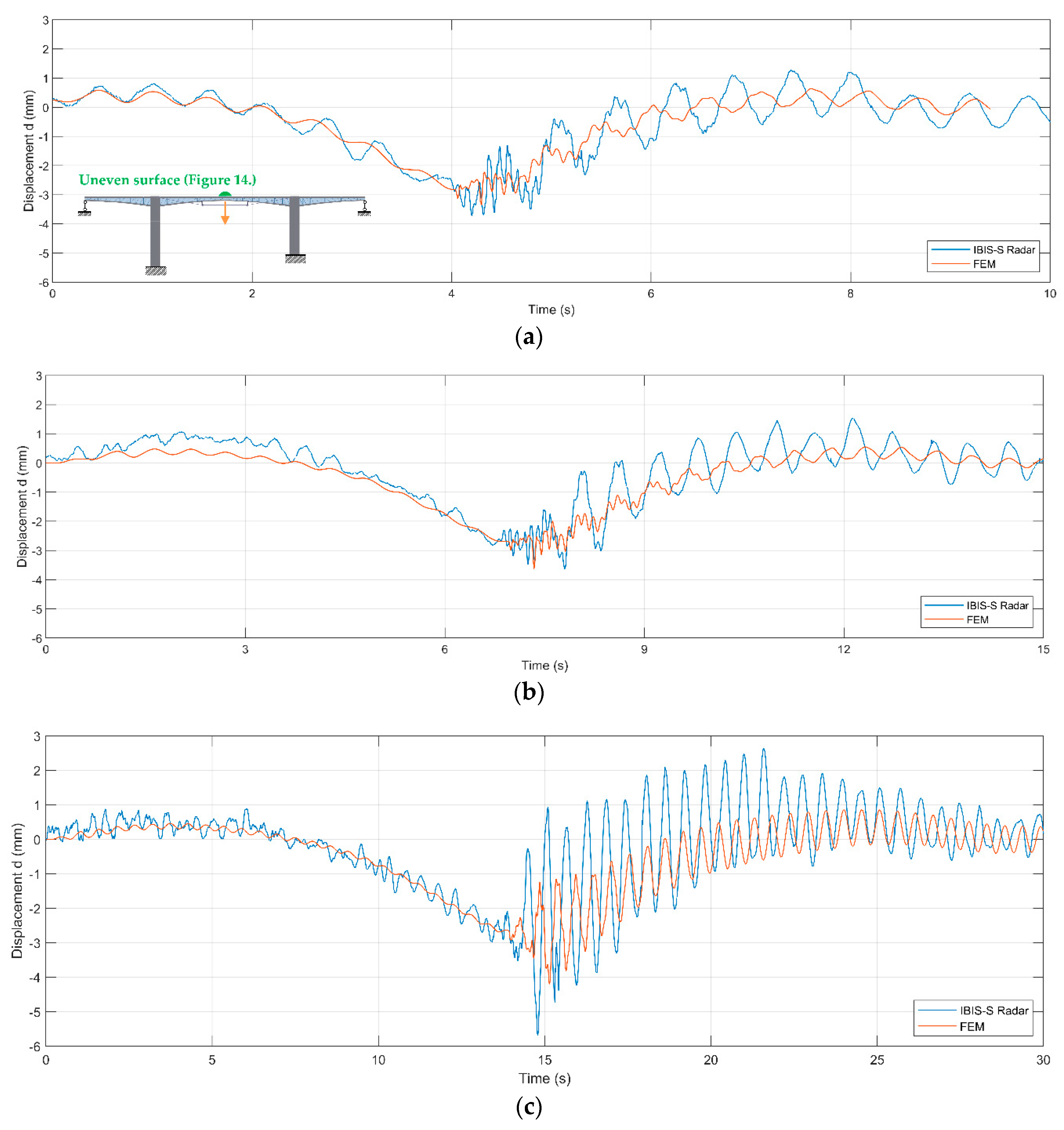
A two-axle truck was used (see Table 3, Truck 1) in the tests. An uneven surface was created by an obstacle placed in the middle of span no. 2 with a length of 0.5 m and a height of 0.06 m (Figure 14). As the axles of the truck hit the uneven surface, significant dynamic effects occurred (Figure 15).
Vertical displacements in the middle of span no. 2 were recorded by the IBIS-S radar. Both recorded and numerical results are presented in Figure 15. The comparison of the obtained results in Figure 15 shows that the overall responses, assuming different vehicle velocities (57, 36 and 21 km/h), of both test and analysis are similar. The most significant dynamic response is caused by the vehicle passing over the obstacle in the middle of span no. 2. The vehicle used during these tests (two-axle truck—Truck 1 from Table 3) had a substantial effect on the overall response. If there are other cars in the traffic flow, they can be also assumed, and the partial effects can be added.
The calculated time histories have slightly smaller dynamic amplitudes than the displacement measurement records. The reason for this could be caused by an inappropriate assumption of the stiffness of the tires (see Table 4). In this case, a rough estimation of tire stiffness was carried out by measuring changes in tire dimensions in the vertical and horizontal directions caused by gravitational forces. Tire pressure identification using sensors could be an option to obtain this data more accurately, as in [28]. This effect should be studied further in the future.
In general, IBIS-S radar allows for the measurement of hundreds of points along the bridge with a sampling rate of up to 200 samples/s. In the case study, results from only two points are presented. Two reflectors were installed (Figure 5b) to achieve better radar signal. The two selected points are those where the displacement measurements needed to be carried out.
7. Evaluation of Axial Forces in Cables
The next comparison between the verified and validated FEM model and measurements concerns the axial forces in the external pre-stressed cables. The values of axial forces Ntest in the cables can be determined from the measured frequencies and geometric and material characteristics of the cables (Table 1) using Equation (4) from [29]:
where f1 is the first natural frequency, L is the length of the cable and μ is weight per meter.
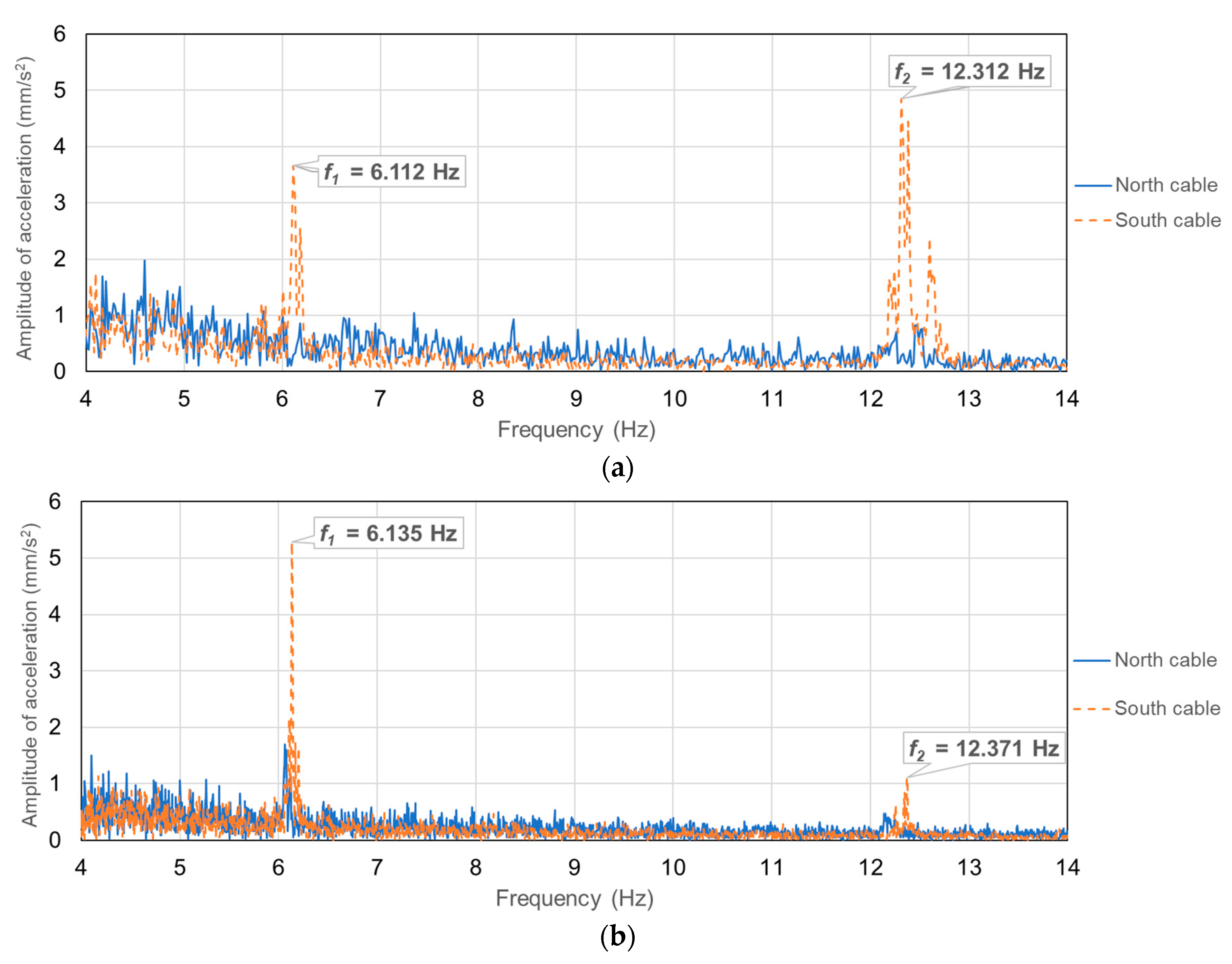
To determine the axial forces Ntest, accelerometers were mounted on two pre-stressed cables (on the northern and southern edge of the bridge, see Figure 4). The first natural frequencies of these cables f1 were found from the dynamic response achieved by using fast Fourier transform (Figure 16). Two situations were considered: an unloaded and a bridge loaded by two heavy trucks (according to Table 3). Both cables have the same geometric and material characteristics (see Table 1 and Table 2), which is proven in Figure 16, where the first and second natural frequencies of both cables are the same.
The length of the cables was considered to be the free length between the deviators (see Table 1). The axial forces were calculated from this data using Equation (3) as follows: Ntest = 2.67 MN for the unloaded bridge and Ntest = 2.69 MN in case of the structure being loaded with two heavy trucks. The difference between them (0.02 MN) matches well with the numerical value calculated as the predicted effect of the applied gravity forces of the load. There is therefore a good reason to believe that the total forces represent their real values on the bridge.
The values of axial forces Ntest and natural frequencies f of the cables can be considered a performance indicator (as in [30]), which can be calculated from the measured data by permanently placed accelerometers to continuously measure the natural frequency. The value presented here for the unloaded bridge will be accounted for as the reference value of the performance indicator. The main benefits of this method are the possibility of measuring during regular traffic without restrictions and evaluating the actual value of the axial force even after years of service.
8. Conclusions
The development of a SHM strategy is presented in this paper using static and dynamic load tests, as well as numerical simulations. Therefore, the results of the tests and simulations of the static and dynamic response of the bridge subjected to traffic loads using a combination of devices, including interferometric radar and a complex measuring system, have been presented in the article. A static load test was performed to verify and validate the FEM model using measured strains and displacements. The combination of devices used is not common, and due to that, acceptable results were obtained from the presented comparisons. To obtain various types of data and to compare the dynamic characteristics, the combination of acceleration and displacement measurements can be used. Accelerometers are more suitable for detecting mode shapes, whereas interferometric radar can help validate numerical models comparing displacements, which are preferred in practice.
A satisfactory numerical model has been prepared. Natural frequencies and MAC values match each other, with the error not exceeding 10%. Structure–vehicle dynamic interactions incorporating uneven surface effects and loss of contact have been derived and used. Numerically predicted dynamic displacements and test results match sufficiently in cases of higher velocity of passing trucks (60 km/h), while the difference of amplitudes is doubled in case of smaller velocities (about 20 km/h). However, the results regarding periods match to each other well. Tire stiffness has to be studied and considered more accurately to improve future results. Deterministically defined loads correspond with real conditions and can be useful not only for the comparison of vibration amplitudes, e.g., accelerations and spectral values, but even for the analysis of dynamic strains and displacements caused by traffic. As shown in this paper, precisely modelled traffic can be used as a comparison tool for future applications of structural health monitoring techniques.
The goal to determine the actual forces in cables has been fulfilled. The presented SHM technique is relatively sensitive, e.g., the weight of only two vehicles could be identified. Moreover, this method provides the specification of the total value of axial force in the cable. Additionally, the natural frequencies of cables measured by accelerometers can be considered a performance indicator. The static and dynamic response of the bridge is similar to the response obtained by the numerical calculations of the FEM model prepared according to the project documentation of the real execution.
Author Contributions
Conceptualization, M.S.; methodology, M.M.; software, M.S., M.V., K.L. and M.M.; validation, M.V., K.L. and M.M.; formal analysis, M.S.; investigation, M.M., M.V. and K.L.; resources, M.M.; data curation, M.V. and K.L.; writing—original draft preparation, M.M., M.S., K.L. and M.V.; writing—review and editing, M.V.; visualization, M.M., K.L. and M.V.; supervision, M.S.; project administration, M.S. and M.V.; funding acquisition, M.S. All authors have read and agreed to the published version of the manuscript.
Funding
This paper was supported by the Grant Agency of the Ministry of Education, Science, Research and Sports of the Slovak Republic VEGA No. 1/0749/19.
Conflicts of Interest
The authors declare no conflict of interest.
References
- Strauss, A.; Frangopol, D.M.; Kim, S. Use of monitoring extreme data for the performance prediction of structures: Bayesian updating. Eng. Struct. 2008, 30, 3654–3666. [Google Scholar] [CrossRef]
- Chang, P.C.; Flatau, A.; Liu, S.C. Review Paper: Health Monitoring of Civil Infrastructure. Struct. Health Monit. 2003, 2, 257–267. [Google Scholar] [CrossRef]
- Strauss, A.; Mandić Ivanković, A.; Matos, J.C.; Casas, J.R. Performance Indicators for Road Bridges—Overview of Findings and Future Progress. In Proceedings of the Value of Structural Health Monitoring for the reliable Bridge Management, Zagreb, Croatia, 2–3 March 2017; pp. 3.1:1–3.1:6. [Google Scholar]
- Martinez, D.; Malekjafarian, A.; Obrien, E.J. Bridge flexural rigidity calculation using measured drive-by deflections. J. Civ. Struct. Health Monit. 2020. [Google Scholar] [CrossRef]
- Fenerci, A.; Øiseth, O. The Hardanger Bridge monitoring project: Long-term monitoring results and implications on bridge design. Procedia Eng. 2017, 199, 3115–3120. [Google Scholar] [CrossRef]
- Wenzel, H.; Pichler, D. Ambient Vibration Monitoring; John Wiley & Sons, Ltd.: Chichester, UK, 2005; ISBN 0470024305. [Google Scholar]
- Wenzel, H. Health Monitoring of Bridges; John Wiley & Sons, Ltd.: Chichester, UK, 2009; ISBN 9780470031735. [Google Scholar]
- Banas, A.; Jankowski, R. Experimental and Numerical Study on Dynamics of Two Footbridges with Different Shapes of Girders. Appl. Sci. 2020, 10, 4505. [Google Scholar] [CrossRef]
- Zhang, B.; Ding, X.; Werner, C.; Tan, K.; Zhang, B.; Jiang, M.; Zhao, J.; Xu, Y. Dynamic displacement monitoring of long-span bridges with a microwave radar interferometer. ISPRS J. Photogramm. Remote Sens. 2018, 138, 252–264. [Google Scholar] [CrossRef]
- Koto, Y.; Konishi, T.; Sekiya, H.; Miki, C. Monitoring local damage due to fatigue in plate girder bridge. J. Sound Vib. 2019, 438, 238–250. [Google Scholar] [CrossRef]
- Xia, Y.; Chen, B.; Zhou, X.-Q.; Xu, Y.-L. Field monitoring and numerical analysis of Tsing Ma Suspension Bridge temperature behavior. Struct. Control. Health Monit. 2012, 20, 560–575. [Google Scholar] [CrossRef]
- Kim, S.-H.; Park, S.Y.; Jeon, S.-J. Long-Term Characteristics of Prestressing Force in Post-Tensioned Structures Measured Using Smart Strands. Appl. Sci. 2020, 10, 4084. [Google Scholar] [CrossRef]
- Guan, H.; Karbhari, V.M. Vibration-Based Structural Health Monitoring of Highway Bridges; Dept. of Structural Engineering, University of California: La Jolla, CA, USA, 2008. [Google Scholar]
- Haardt, P.; Holst, R. The Value of Structural Health Monitoring for the reliable Bridge Management Monitoring during life cycle of bridges to establish performance indicators. In Value of Structural Health Monitoring for the reliable Bridge Management, Proceedings of the IABSE WC1 WORKSHOP the Value of Structural Health Monitoring for the reliable Bridge Management, Zagreb, Croatia, 2–3 March 2017; Faculty of Civil Engineering, University of Zagreb: Zagreb, Croatia, 2017; pp. 1–9. [Google Scholar]
- Brincker, R.; Ventura, C.E. Introduction. In Introduction to Operational Modal Analysis; John Wiley & Sons, Ltd.: Chichester, UK, 2015; pp. 1–16. ISBN 9781118535141. [Google Scholar]
- Thacker, B.H.; Doebling, S.W.; Hemez, F.M.; Anderson, M.; Pepin, J.; Rodriguez, E. Concepts of Model Verification and Validation; Los Alamos National Lab: Los Alamos, NM, USA, 2004. [Google Scholar] [CrossRef] [Green Version]
- Zhang, L.; Zhao, H.; Obrien, E.J.; Shao, X.; Tan, C. The influence of vehicle–tire contact force area on vehicle–bridge dynamic interaction. Can. J. Civ. Eng. 2016, 43, 769–772. [Google Scholar] [CrossRef]
- Kanda, V. Reconstruction of the Bridge II/547 020 Ružín. Available online: www.asb.sk/stavebnictvo/inzinierske-stavby/mosty/rekonstrukcia-mosta-ii-547-020-ruzin (accessed on 12 April 2019).
- SSC Results of National Traffic Census in Slovak Republic in 2015. Available online: www.ssc.sk/files/documents/dopravne-inzinierstvo/csd_2015/ke/scitanie_vuc_ke_2015.pdf (accessed on 12 April 2019).
- British Standard. Eurocode 8: Design of Structures for Earthquake Resistance—Part 2: Bridges; European Committee for Standardization: Brussels, Belgium, 2010. [Google Scholar]
- Venglar, M.; Milan, S.; Ároch, R.; Budaj, J. Initial Experimental Test of the Port Bridge for Structural Health Monitoring. Appl. Mech. Mater. 2016, 837, 135–139. [Google Scholar] [CrossRef]
- Alani, A.M.; Aboutalebi, M.; Kilic, G. Use of non-contact sensors (IBIS-S) and finite element methods in the assessment of bridge deck structures. Struct. Concr. 2014, 15, 240–247. [Google Scholar] [CrossRef]
- Gentile, C. Application of Radar Technology to Deflection Measurement and Dynamic Testing of Bridges. In Radar Technology; Kouemou, G., Ed.; IntechOpen: Rijeka, Croatia, 2010. [Google Scholar]
- Reynders, E.; Degrauwe, D.; De Roeck, G.; Magalhães, F.; Caetano, E. Combined Experimental-Operational Modal Testing of Footbridges. J. Eng. Mech. 2010, 136, 687–696. [Google Scholar] [CrossRef]
- Peeters, B. System Identification and Damage Detection in Civil Engineering. Ph.D. Thesis, KU Leuven, Leuven, Belgium, 2000. [Google Scholar]
- Peeters, B.; Lau, J.; Lanslot, J.; van der Auweraer, H. Automatic modal analysis-Myth or reality? Sound Vib. 2008, 42, 17. [Google Scholar]
- Rosso, C.; Bonisoli, E.; Bruzzone, F. Could the veering phenomenon be a mechanical design instrument? In Topics in Modal Analysis & Testing; Conference Proceedings of the Society for Experimental Mechanics Series; Mains, M., Blough, J.R., Eds.; Springer International Publishing: Cham, Switzerland, 2017; Volume 10, pp. 85–95. ISBN 9783319548098. [Google Scholar]
- Zhu, B.; Han, J.; Zhao, J. Tire-Pressure Identification Using Intelligent Tire with Three-Axis Accelerometer. Sensors 2019, 19, 2560. [Google Scholar] [CrossRef] [PubMed] [Green Version]
- Clough, R.W.; Penzien, J. Dynamics of Structures; McGraw-Hill: New York, NY, USA, 1993; ISBN 9780071132411. [Google Scholar]
- Furtmüller, T.; Adam, C. Compensation of Temperature Effects in Long-Term Monitoring of a Highway Bridge located in the Austrian Alps. Procedia Eng. 2017, 199, 2078–2083. [Google Scholar] [CrossRef]
Figure 1.
The bridge over Ružín Dam: (a) photo; (b) side-view; (c) cross-sections (dimensions in millimeters).
Figure 1.
The bridge over Ružín Dam: (a) photo; (b) side-view; (c) cross-sections (dimensions in millimeters).

Figure 2.
The reinforcement of the joint in the middle of the span no. 2 with external pre-stressed cables [18].
Figure 2.
The reinforcement of the joint in the middle of the span no. 2 with external pre-stressed cables [18].

Figure 3.
(a) The FEM model of the structure with (b) the passing truck (dimensions in millimeters); (c) detail A—determination of contact.
Figure 3.
(a) The FEM model of the structure with (b) the passing truck (dimensions in millimeters); (c) detail A—determination of contact.

Figure 4.
The measurement setup (a) top view; (b) side-view; (c) cross-section in the middle of span no. 2 (dimensions in millimeters).
Figure 4.
The measurement setup (a) top view; (b) side-view; (c) cross-section in the middle of span no. 2 (dimensions in millimeters).


Figure 5.
The Interferometric radar (a) IBIS-S device; (b) radar placement for the measurements.

Figure 6.
Projection of the measured displacement.

Figure 7.
The displacement in the middle of span no. 2 caused by two heavy trucks (a) IBIS-S radar measurement; (b) results from FEM model.
Figure 7.
The displacement in the middle of span no. 2 caused by two heavy trucks (a) IBIS-S radar measurement; (b) results from FEM model.

Figure 8.
The strains in the middle of span no. 2 caused by two heavy trucks (a) measurement by strain gauges; (b) results from FEM model.
Figure 8.
The strains in the middle of span no. 2 caused by two heavy trucks (a) measurement by strain gauges; (b) results from FEM model.


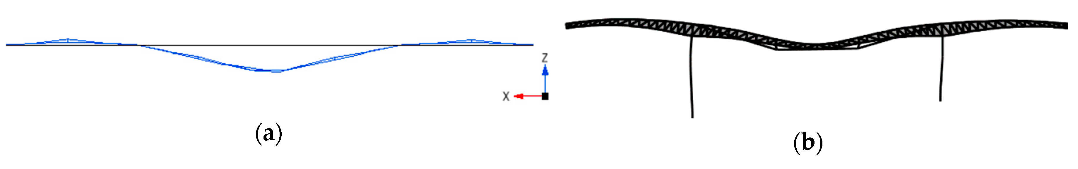
Figure 9.
The 3rd identified mode shape (a) measurement, (b) FEM model.

Figure 10.
The 5th identified mode shape (a) measurement, (b) FEM model.

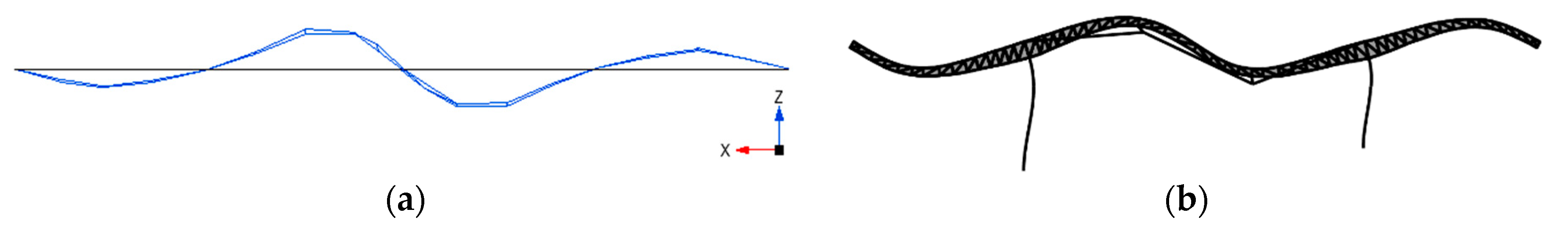
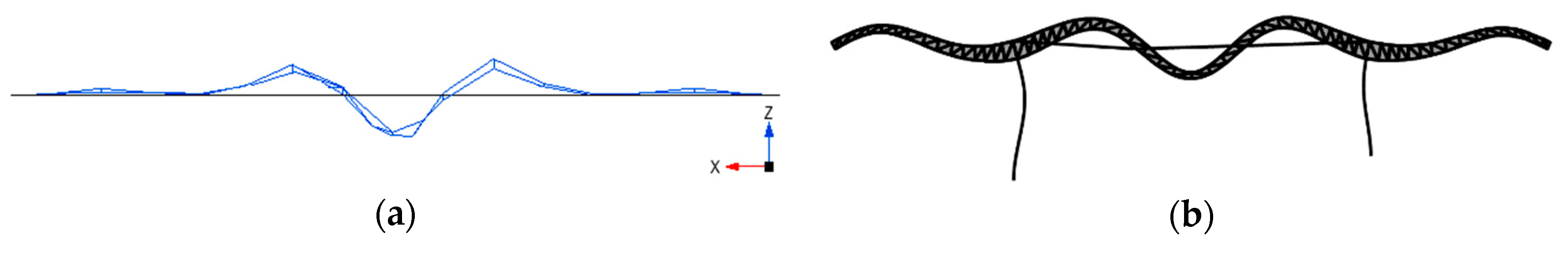
Figure 11.
The 7th identified mode shape (a) measurement, (b) FEM model.

Figure 12.
The 10th identified mode shape (a) measurement, (b) FEM model.

Figure 13.
Displacement record by IBIS-S radar in the middle of span no. 2—the 3rd frequency.

Figure 14.
Artificial uneven surface placed in the middle of the span no. 2 (a) photo; (b) dimensions in millimeters (R—radius).
Figure 14.
Artificial uneven surface placed in the middle of the span no. 2 (a) photo; (b) dimensions in millimeters (R—radius).

Figure 15.
Displacement records in the middle of span no. 2. (a) Velocity 57 km/h; (b) velocity 36 km/h; (c) velocity 21 km/h.
Figure 15.
Displacement records in the middle of span no. 2. (a) Velocity 57 km/h; (b) velocity 36 km/h; (c) velocity 21 km/h.

Figure 16.
The response spectra of the cables. (a) Unloaded bridge; (b) loaded bridge (f1—1st natural Figure 2. nd natural frequency).
Figure 16.
The response spectra of the cables. (a) Unloaded bridge; (b) loaded bridge (f1—1st natural Figure 2. nd natural frequency).


Table 1.
Geometric and material characteristics of strand (LS15.7/1860 MPa).
| Nominal Diameter Φ | Tensile Strength Fpk | Area of Cross-Section Astrand | Weight per Meter μstrand | Young Modulus of Elasticity E |
|---|---|---|---|---|
| 15.7 mm | 1860 MPa | 150 mm2 | 1.18 kg/m | 190 GPa |
Table 2.
Geometric and material characteristics of cable (15 pieces of strand LS15.7/1860 MPa).
| Length between Deviators L | Area of Cross-Section of 15 Strands Asteel | Area of Cross-Section of Grout Agrout | Area of Cross-Section of Duct Aduct | Weight per Meter μ |
|---|---|---|---|---|
| 24.36 m | 2250 mm2 | 5000 mm2 | 1700 mm2 | 30.12 kg/m |
Table 3.
Characteristics of vehicles (weight) according to the measurement before the test.
| Truck 1 | Truck 2 | |
|---|---|---|
| Front axle | 7720 kg | 7280 kg |
| Rear axle | 10,620 kg | 10,550 kg |
| In total | 18,340 kg | 17,830 kg |
Table 4.
Characteristics of axles—Truck 1.
| Axle | Spring Characteristics | Damping Characteristics | Unbalanced Axle Mass | Balanced Mass over Axle | Tire Stiffness |
|---|---|---|---|---|---|
| Front | 517 kN/m | 23 kN/(m/s) | 1300 kg | 6420 kg | 100 MN/m |
| Rear | 1322 kN/m | 130 kN/(m/s) | 3000 kg | 7620 kg | 150 MN/m |
Table 5.
Average temperatures during the measurement.
| Air | Span no. 1 | Span no. 2 (Main) | Span no. 3 |
|---|---|---|---|
| 21.6 °C | 21.9 °C | 22.1 °C | 22.0 °C |
Table 6.
Comparison of natural frequencies and mode shapes.
| No. | Mode Shape (Direction) | Natural Frequency (Measured) | Natural Frequency (Calculated) | Cross-MAC (Modal Assurance Criterion) | Figure |
|---|---|---|---|---|---|
| 1 | Global in X direction | N/A 1 | 1.16 | N/A1 | N/A 1 |
| 3 | Global in Z direction | 1.71 | 1.76 | 0.99 | Figure 9 |
| 5 | Global in Z direction | 3.78 | 3.50 | 0.93 | Figure 10 |
| 7 | Global in Z direction | 5.21 | 5.33 | 0.94 | Figure 11 |
| 10 | Global in Z direction | 8.27 | 7.9 | 0.92 | Figure 12 |
1 N/A—not available from measurements.
© 2020 by the authors. Licensee MDPI, Basel, Switzerland. This article is an open access article distributed under the terms and conditions of the Creative Commons Attribution (CC BY) license (http://creativecommons.org/licenses/by/4.0/).
Share and Cite
MDPI and ACS Style
Sokol, M.; Venglár, M.; Lamperová, K.; Márföldi, M. Performance Assessment of a Renovated Precast Concrete Bridge Using Static and Dynamic Tests. Appl. Sci. 2020, 10, 5904. https://0-doi-org.brum.beds.ac.uk/10.3390/app10175904
AMA Style
Sokol M, Venglár M, Lamperová K, Márföldi M. Performance Assessment of a Renovated Precast Concrete Bridge Using Static and Dynamic Tests. Applied Sciences. 2020; 10(17):5904. https://0-doi-org.brum.beds.ac.uk/10.3390/app10175904
Chicago/Turabian StyleSokol, Milan, Michal Venglár, Katarína Lamperová, and Monika Márföldi. 2020. "Performance Assessment of a Renovated Precast Concrete Bridge Using Static and Dynamic Tests" Applied Sciences 10, no. 17: 5904. https://0-doi-org.brum.beds.ac.uk/10.3390/app10175904
Note that from the first issue of 2016, this journal uses article numbers instead of page numbers. See further details here.