Article

Application of Fuzzy Theory and Optimum Computing to the Obstacle Avoidance Control of Unmanned Underwater Vehicles

Mechanical and Aerospace Engineering, National Defense University, Tahsi, Taoyuan 33509, Taiwan
*
Author to whom correspondence should be addressed.
Submission received: 12 August 2020 / Revised: 28 August 2020 / Accepted: 28 August 2020 / Published: 2 September 2020
(This article belongs to the Special Issue Underwater Vehicles)

Abstract

:
Autonomous underwater vehicles and remotely operated vehicles (ROVs) are unmanned underwater vehicles widely used in marine environments. Establishing an efficient obstacle avoidance approach in underwater environments remains a challenge for these vehicles. Most studies have relied on simulated results; few have been conducted with vehicles in a real environment. This study used an ROV equipped with a scanning sonar as an experimental platform and applied fuzzy logic control to solve nonlinear and uncertain problems, which are difficult to address using conventional control theory. Using data from the depth and inertial sensors, fuzzy logic control can output defuzzification command values that are passed through a fuzzy inference engine to control ROV motion. Fuzzy logic control was used to evaluate depth and heading degrees in navigation experiments. In heading navigation, scanning sonar was used to detect obstacles in the scanning range. An optimum navigation strategy was also developed to calculate appropriate headings to safely and stably navigate during a mission to attain a predetermined destination. The results indicated that the ROV with fuzzy logic control had superior control stability and obstacle avoidance in an underwater environment.

1. Introduction

Unmanned underwater vehicles (UUVs) are generally divided into autonomous underwater vehicles (AUVs) and remotely operated vehicles (ROVs). AUVs are most frequently used for monitoring and scanning the ocean surface because of their high speed and autonomous capabilities [1]. Marine scientists routinely use ROVs to collect deep-sea data and samples. The avoidance of risks through human intervention in deep-sea research and exploration is an evident advantage of using ROVs, and remote operation allows numerous scientists and engineers to discuss incoming data and make collective decisions on operations from a shipboard control van [2].
In the development of UUVs, a suitable structural design and suitable motion control are the primary concerns, as is obtaining a general mathematical model for describing a complex, random, and nonlinear marine environment. Conventional control methods, such as proportional–integral–derivative (PID) control, are unsuitable, and finding a control method for an uncertain environment is necessary.
At present, the commonly used methods for the navigation control of underwater vehicles are PID control, adaptive control, fuzzy logic control (FLC), and neural network control. To control UUVs, Hassanein [3] applied fuzzy theory to the environmental adaptation problem and compared it with a traditional mathematical model of control for depth and heading control. Anirban [4] simulated a PID controller that met the expected depth control value. Shi et al. [5] used an adaptive neural–fuzzy inference system for the depth control of an AUV. The system could adjust the fuzzy rule parameters by itself instead of requiring artificial adjustment. Wang et al. [6] considered the most prominent advantages of FLC, further optimized by a genetic algorithm. Joo [7] considered a controller composed of a linear–quadratic regulator (LQR) controller to maintain zigzag vertical movement for gliding and towing (proportional plus derivative) PD controllers to control elevator/rudder angles. Lin et al. [8] designed an adaptive fuzzy stabilization controller for an underactuated surface vessel in the presence of unknown time-varying environmental disturbances and input saturation. Makavita et al. [9] reported the results of an experimental study conducted to compare the performances of different adaptive control methods for the depth control of a UUV, which represents a significant challenge compared with heading control due to increased noise, time delay, and thrust requirements. Bui and Kim [10] used an FLC method that enabled AUVs to navigate safely through obstacles to a goal, with the optimal path proven by their simulation results. Shimmin et al. [11] devised a self-tuning fuzzy controller for application in submerged ROVs. In simulations, the vehicle exhibited a generally conservative and safe behavior during the training period, as is required in real-time on-site applications. Some studies have used scanning sonar to assist with the motion control of UUVs. Wang et al. [12] and Sebastián [13] used the artificial potential field concept to avoid obstacles. Subramanian et al. [14] provided an obstacle avoidance algorithm that generated path elements to the trajectory planner, and the vehicle tracked the trajectory [12,13,14] using the potential field computation to avoid obstacles. Only computer simulations were performed. Once the pre-set obstacle had been detected, the vehicle directly moved around and passed the obstacle in order to complete the simulation. However, in a real environment the vehicle could not complete such movement without considering the vehicle control. Braginsky and Guterman [15] presented a scanning sonar with a seabed gradient detection technique that could predict seabed and attitude changes. Grefstad and Schjølberg [16] designed a vehicle-fixed occupancy grid method to plan an optimal path around obstacles [15,16] using the image processing approach to identify the obstacles. It is not suitable to apply to UUVs, though, because the image processing uses lots of computing resources and the energy consumption could be large.
This study used an ROV to analyze vehicle movement, heading in degrees, and altitude data through the use of sensors. FLC used sensor data to navigate the ROV and enabled the vehicle to self-adjust the motor power compensation output. Using scanning sonar with optimum value computing enabled successful avoidance of obstacles, and the ROV could pass through them to the target.

2. Materials and Methods
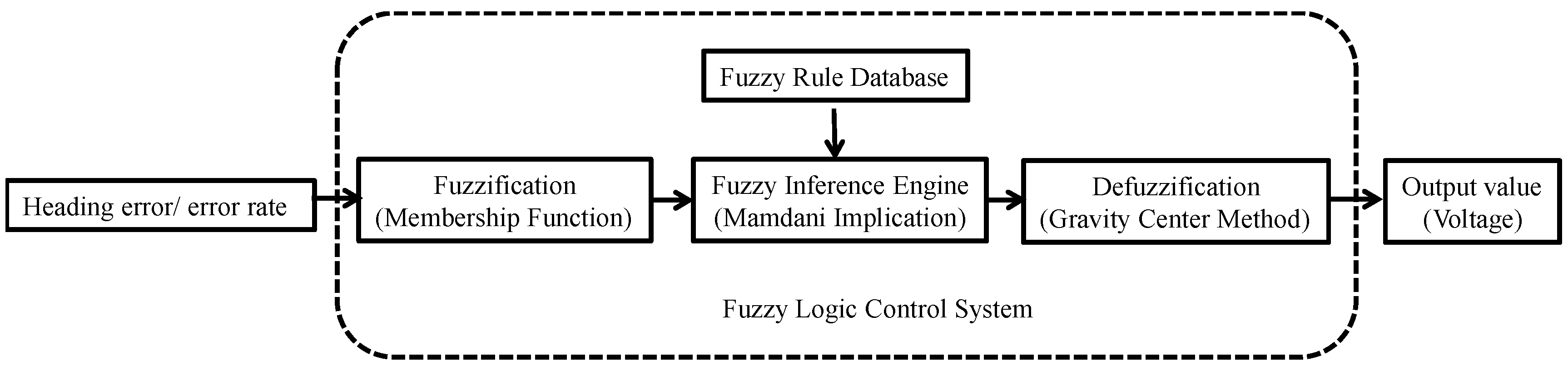
Sensor data from a voltage-type water pressure gauge (the red oval in Figure 1) and an inertial measurement unit (IMU) sensor (the blue oval in Figure 1) were collected using a data acquisition module. The IMU sensor included a gyroscope (ITG3205 chip), an accelerometer (ADXL345 chip), and a digital compass (HMC5883L chip) with a 0.5 s sampling time. By using these sensors, yaw, roll, and pitch information for the ROV was obtained. During experiments, the depth of the ROV was kept as a constant and heading information was entered as input parameters to the FLC. The scanning sonar (the green oval in Figure 1) emitted a beam in different directions of an angular sector, with a frequency centered at 650 kHz and a range between 0.5 m and 60 m. The beam had a horizontal width of 2.4° and a vertical width of 40° with a 3 s sampling time.

2.1. FLC

Figure 2 presents the flowchart of the FLC. The heading error and heading error rates were obtained using the IMU sensor and water pressure gauge. Before these data were inputted into the fuzzy inference engine, they were passed through the fuzzification process by using triangular membership functions. The fuzzy rule database was also defined for the inference engine. Finally, the output values were calculated through defuzzification, based on which the ROV propeller was driven. Detailed descriptions are provided as follows.
For fuzzification, triangular and trapezoidal membership functions were defined as follows [17]:
A ( x ) = { b ( 1 | x a | s ) 0 ,   o t h e r w i s e ,   a s x   a + s   F o r   t r i a n g u l a r .
A ( x ) = { ( a x ) e a b ,   w h e n   a x b e ,   when   b x c ( d x ) e d c ,   w h e n   c x d 0 ,   o t h e r w i s e   F o r   t r a p e z o i d a l .
The parameters a, b, and s of the triangular function are portrayed in Figure 3a: a value a, a distance s, a membership function value b, a lower limit a s , and an upper limit a + s . The parameters a, b, c, d, and e of the trapezoidal function are portrayed in Figure 3b similarly.
Using the triangular membership function, two parameters—heading error and heading error rate—were defined as input functions. Figure 4a presents 12 membership functions for the heading error: right zero (zero), right very small (RVS), right small (RS), right medium (RM), right big (RB), right very big (RVB), left very big (LVB), left big (LB), left medium (LM), left small (LS), left very small (LVS), and left zero (Zero). Membership functions for the heading error rate are presented in Figure 4b.
In the fuzzy rule database, the “if–then” format was used to specify the relations between input and output values. Table 1 presents the fuzzy rule database of heading control for the ROV horizontal propeller. The heading error had 12 membership functions—RVB, RB, RM, RS, RVS, zero, Zero, LVS, LS, LM, LB, and LVB—and heading error rate had nine membership functions—LB, LM, LS, LVS, Zero, RVS, RS, RM, and RB. This resulted in 108 rules in the fuzzy logic database (Table 1). For example, if the heading error was RS and the heading error rate was LS, then the velocity of the horizontal propeller was LVS.
Generally, the Mamdani implication method is used for fuzzy inference. When μ A ( x ) and μ B ( x ) are the minimum membership values, they can be mathematically represented as follows:
μ C ( x ,   y ) = m i n ( μ A ( x ) ,   μ B ( y ) ) .
Therefore, defuzzification was performed using the following gravity center:
Z * = i 1 k Z i B ( Z i ) i 1 k B ( Z i ) ,
where Z * is the explicit output value after defuzzification and B ( Z i ) is the output value from fuzzy inference. The output value Z i denotes the position of the center of gravity of the fuzzy inference.
Figure 5 illustrates the heading error surfaces as outputs from the FLC. Coordinate axes are inputs and outputs. The heading error and error rate were used as inputs, which were sensed using ROV sensors, and inferences were generated using fuzzy logic. The output value from the controller represented the voltage of propeller motors on the ROV. Moreover, the ROV used four propellers and two sets of bidirectional controls to regulate the horizontal motor for rotating in forward, reverse, left, and right directions. The red axis of the origin of the surface indicated the initial values of the control. A steeper gradient near the origin point indicated that values were more sensitive for the control system.

2.2. Optimum Value Computing

Optimization techniques were used to obtain an improved solution under given conditions. In this study, obstacle avoidance control was helpful. The general optimal control problem can be formulated as follows [18]: Find an n-vector x = ( x 1 ,   x 2 , , x n ) of design variables to minimize a vector objective (cost) function
F ( x ) = [ f 1 ( x ) ,   f 2 ( x ) , , f n ( x ) ]
subject to the equality constraints
h j ( x ) = 0 ,   j = 1 ,   2 , , p
and the inequality constraints
g i ( x ) 0 ,   i = 1 ,   2 ,   ,   m ,
where h j ( x ) are the equality constraints and g i ( x ) are the inequality constraints. The objective functions are criteria for evaluating designs. For an obstacle avoidance approach, certain limitations (i.e., constraints) and design variables cannot be selected completely freely. Equality and inequality constraints are often required for an approach.

2.2.1. Problem Definition

  • Choosing design variables: Based on the requirements of the approach, the user can choose factors as design variables. These can be varied during the optimization iteration process. Other factors are treated as constants. In this study, the chosen design variables for the obstacle avoidance approach were the number of points on the radius of the scanning sonar ( P i , i = 1 , 2 , , n ), the radius of the scanning sonar ( R x , R y ) , and the sector of the scanning sonar (θ) (Figure 6).
  • Defining an objective function: The objective function must be defined according to the purpose and requirements of the approach. The objective function in this study was defined as the direction of movement (DM) of the ROV:
    minimize   D M ( P i , R x , R y , θ ) = C D e s ( i ) + C O b s ( i ) j ,
    C D e s ( i ) = 1 D ( i ) = 1 ( X D e s X i ) 2 + ( Y D e s Y i ) 2 ,
    and
    C O b s ( i ) j = 1 d ( i , j ) = 1 ( X O b s ( j ) X i ) 2 + ( Y O b s ( j ) Y i ) 2 ,
    where D ( i ) represents the distance between point P and the destination, and d ( i , j ) represents the distance between point P and the obstacle. C D e s ( i ) indicates the negative inverse value of D ( i ) , and C O b s ( i ) j indicate the positive inverse value of d ( i , j ) due to the presence of n obstacles detected. If the minimum value of DM is located at point “i”, the ROV should turn to point “i” and move forward.
  • Identifying constraints: Assuming that R is the radius of the scanning sonar, θ indicates the scanning area for the forward motion. Suggested ranges of the mentioned design variables are summarized as follows:
    R     R x   R ,
    0     R y   R ,
    and
    90 °     θ     90 ° .

2.2.2. Optimal Control Process

The calculation process is depicted in Figure 7. The following sequence of steps was performed:
  • Initialization of the ROV in the destination heading in degrees and the setting of a semicircular region of radius R centered at the ROV point.
  • Execution of obstacle avoidance when an obstacle was detected.
  • Computation of the lowest cost function value and its heading degree.
  • Use of the fuzzy logic controller to make the ROV change its current heading degree to the cost function heading (degree) to avoid the obstacle.
  • Updating of the ROV’s position.
In Figure 8a, the destination and the obstacle are aligned, whereas in Figure 8b, they are not. In total, seven points (n = 7) exist on the radius of the scanning sonar, and θ is 120°. For each of the points, the value of the cost function was calculated. In Figure 8a, point “1” and point “7” have the lowest cost values; therefore, the ROV would move forward in the direction of either point “1” or point “7”. In Figure 8b, point “1” has the lowest cost value; the ROV should turn toward point “1” when the destination and the obstacle are not aligned. In the following experiments, the destination is assumed to be a virtual point ahead of the ROV (5 m, maximum range of the scanning sonar) in the target heading direction.

2.2.3. Simulation of Single Obstacle Avoidance

Figure 9 presents the simulation results of the obstacle avoidance approach. The red line indicates the trajectory of the ROV with the result of obstacle avoidance by optimum value computing. The heading (degree) of the destination is defined as the north of the map. The ROV started toward the destination from origin point (0, 0). At point “a”, an obstacle was detected and the ROV turned right 60° to avoid the obstacle. At point “c”, no obstacle was detected, and the ROV traveled toward the destination.
Figure 10 presents the cost function values of optimum value computing. As shown in Figure 10, 7 points were defined as follows: −60° (red), −40° (orange), −20° (yellow), 0° (green), 20° (sky blue), 40° (navy blue), and 60° (purple). The total time of the simulation was 42 s. According to Equations (8) and (9), the cost function values of the destination and obstacle were negative and positive, respectively. Therefore, the sum of the cost function values from Equation (7) was negative, which meant that no obstacles were present inside the range of the scanning sonar, and the ROV traveled toward the destination. The ROV traveled toward the destination from 0 s to 17 s. At 17 s, point “a”, an obstacle was detected, and the cost function values suddenly changed from negative to positive. The maximum value was 0.0009 for −60° (red line), and the minimum value was 0.00055 for 60° (purple line). This meant that the obstacle was located to the left of the ROV, and it should turn right to avoid it. This situation continued from 17 s to 24 s. At 20 s, point “b”, the cost function values were updated again because the ROV was nearing the obstacle and the maximum value had changed from −60° (red line) to −20° (yellow line). However, the minimum value, 0.0015, remained at 60° (purple line), and the ROV continued to travel in the direction of 60°. Finally, no obstacle was detected (at point “c”). The cost function values became negative again, and the ROV turned to move toward the destination.
In the simulated result, the obstacle avoidance approach successfully enabled the ROV to avoid the obstacle. Next, we used the approach in an experiment with multiple obstacles in a real environment.

3. Results

3.1. Experimental Results of Heading Control

The depth of the multiheading control was 0.5 m to ensure that the cable did not interfere with the ROV’s motion.
The ROV initially began with a heading of 22° and was driven forward for 20 s. The ROV then turned clockwise toward the subsequent target heading of 52°. The heading was maintained at 52° for 20 s. The ROV then turned clockwise to the third target heading of 95° and locomoted for 55 s. The root mean square error (RMSE) values of the multiheading control were calculated as shown in Equation (14), where x i indicates the data points (heading), xtarget indicates the target heading, and n indicates the total number of data points.
RMSE = ( x i x t a r g e t ) 2 n
The RMSE values for the multiheading control headings of 22°, 55°, and 95° were 4.7, 2.06, and 3.09, respectively.
Figure 11 presents the multiheading control result, with all yaw situations for the target headings. In the heading control experiment, the yaw phenomenon caused by the hydrodynamic inertial force resulted in unsatisfactory performance of the FLC. The effect of the rotational motion of the ROV on the maneuvering of the FLC was more significant than the translational motion of the ROV. When the FLC adjusted the heading of the ROV to the target degree, it could command different output powers of the horizontal motors that generated the rotational motion (i.e., yaw) of the ROV. However, the vertical motors did not possess this. The heading control of the ROV was coupled with translational and rotational motions. This control was too complex for the FLC commanding the ROV’s motion.

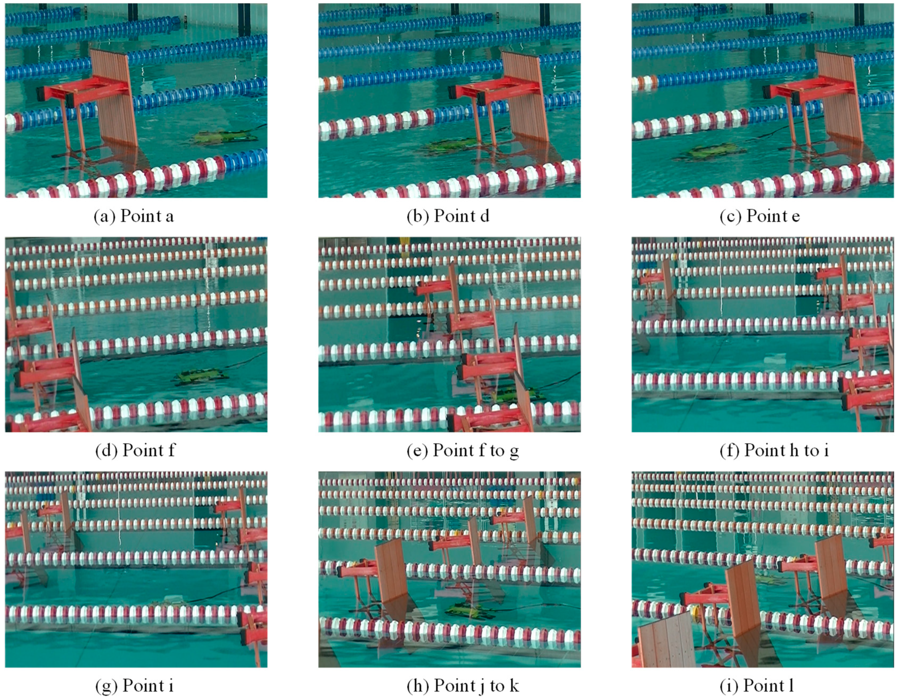
3.2. Experimental Results of the Obstacle Avoidance Approach

Figure 12 presents the experimental results of the ROV’s multiple obstacle avoidance. The obstacles are identified by purple upper-case letters, the points of the scan map are marked by blue lower-case letters, and the red line signifies the trajectory of the ROV with the results of obstacle avoidance by optimum value computing. In the obstacle avoidance experiment, the target heading was due north according to the map orientation, and the radius R of the obstacle avoidance approach was 1.7 m. The ROV started toward the destination at point “a”. From point “b” to point “d”, the ROV successfully avoided the first obstacle. Between points “d” and “e”, the ROV continued to travel toward the destination. From point “e” to point “g”, the ROV smoothly avoided the middle row of obstacles “B” and “C”. At point “g”, the third row of obstacles, “D”, “E”, and “F”, was detected. The ROV chose to turn right 60° and traveled between obstacles “E” and “F” from point “h” to point “k”. Finally, the ROV again traveled toward the destination from point “l”.
Figure 13 presents the cost function values of optimum value computing. In total, seven points were defined as simulation parameters. The total time of the ROV obstacle avoidance experiment was 96 s. The lowest cost function values made the ROV change direction to avoid the obstacles. As shown in Figure 13, obstacles were avoided three times by the ROV. At 14 s to 26 s, the ROV turned right 60° because the point at 60° (purple) was calculated as having the lowest value of the cost function. After passing around obstacle “A”, the middle row of obstacles made the ROV turn left 60°, because the point for −60° (red) had the lowest cost function value. Finally, the third row of obstacles made the ROV turn right 60° again on the basis of the cost function for 60° (purple). Figure 14 reproduces images of the scanning sonar. Figure 15 presents the side view images of the experiments.

4. Conclusions

In an underwater environment with nonlinear and unpredictable characteristics, establishing an accurate mathematical model using conventional control theory is difficult. Therefore, this study used the FLC method with its high adaptability and tolerance of partial uncertainty to control a UUV’s motion.
According to the experimental results, the ROV with the FLC and sonar sensor exhibited the following performances for heading control and obstacle avoidance:
  • For heading control in the experiment, the FLC system directly commanded the ROV’s motion according to the data sensed in the environment. It reduced dependence by using the vehicle’s motion and environment models.
  • Implementation of the heading control was more difficult because of the evident hydrodynamic force generated by the ROV’s motors, which caused a yaw phenomenon. The FLC required time to stabilize the ROV.
  • In the obstacle avoidance experiment, the sonar sensor with optimum value computing combined with fuzzy logic control allowed for efficient avoidance of the obstacles and movement to the target destination. This would be helpful for the navigation control of UUVs.
In this study, the performance of the external sensor on the ROV was evaluated using an experiment that provided a basis for further development of AUV design.

Author Contributions

S.C. conceived the experiments and drafted the manuscript; T.L. reviewed and revised the manuscript; K.J. and C.W. provided experimental data. All authors have read and agreed to the published version of the manuscript.

Funding

This research was funded by Ministry of Education Taiwan under grant numbered 1090023205C.

Acknowledgments

The authors would like to acknowledge the CAD/CAM team’s members in NDU who contributed and helped in the experiment.

Conflicts of Interest

The authors declare no conflict of interest.

References

  1. Nørve Eidsvik, O.A.; Schjølberg, I. Finite element cable-model for Remotely Operated Vehicles (ROVs) by application of beam theory. Ocean. Eng. 2018, 163, 322–336. [Google Scholar] [CrossRef] [Green Version]
  2. Humphris, S.E. Vehicles for Deep Sea Exploration. In Elements of Physical Oceanography: A Derivative of the Encyclopedia of Ocean Sciences; Steele, J.H., Thorpe, S.A., Thompson, K.K., Eds.; Elsevier Ltd.: Boston, MA, USA, 2009; pp. 197–210. [Google Scholar]
  3. Hassanein, O.; Anavatti, S.G.; Ray, T. On-line adaptive fuzzy modeling and control for autonomous underwater vehicle. In Recent Advances in Robotics and Automation; Springer: Berlin/Heidelberg, Germany, 2013; pp. 57–70. [Google Scholar]
  4. Nag, A.; Patel, S.S.; Akbar, S.A. Fuzzy logic based depth control of an autonomous underwater vehicle. In Proceedings of the 2013 International Mutli-Conference on Automation, Computing, Communication, Control and Compressed Sensing, Kottayam, Kerala, India, 22–23 March 2013; pp. 117–123. [Google Scholar]
  5. Shi, X.; Chen, J.; Yan, Z.; Li, T. Design of AUV height control based on adaptive Neuro-fuzzy inference system. In Proceedings of the 2010 IEEE International Conference on Information and Automation, Harbin, China, 20–23 June 2010; pp. 1646–1651. [Google Scholar]
  6. Chen, J.W.; Zhu, H.; Zhang, L.; Sun, Y. Research on fuzzy control of path tracking for underwater vehicle based on genetic algorithm optimization. Ocean. Eng. 2018, 156, 217–223. [Google Scholar] [CrossRef]
  7. Joo, M.G. A controller comprising tail wing control of a hybrid autonomous underwater vehicle for use as an underwater glider. Int. J. Nav. Archit. Ocean. Eng. 2019, 11, 865–874. [Google Scholar] [CrossRef]
  8. Lin, X.; Nie, J.; Jiao, Y.; Liang, K.; Li, H. Adaptive fuzzy output feedback stabilization control for the underactuated surface vessel. Appl. Ocean. Res. 2018. [Google Scholar] [CrossRef]
  9. Makavita, C.D.; Jayasinghe, S.G.; Nguyen, H.D.; Ranmuthugala, D. Experimental Study of a Command Governor Adaptive Depth Controller for an Unmanned Underwater Vehicle. Appl. Ocean. Res. 2019. [Google Scholar] [CrossRef]
  10. Bui, L.D.; Kim, Y.G. An obstacle-avoidance technique for autonomous underwater vehicles based on BK-products of fuzzy relation. Fuzzy Sets Syst. 2006, 157, 560–577. [Google Scholar] [CrossRef]
  11. Shimmin, D.W.; Stephens, M.; Swainston, J.R. Adaptive control of a submerged vehicle with sliding fuzzy relations. Fuzzy Sets Syst. 1996, 79, 15–24. [Google Scholar] [CrossRef]
  12. Wang, D.; Wang, P.; Zhang, X.; Guo, X.; Shu, Y.; Tian, X. An obstacle avoidance strategy for the wave glider based on the improved artificial potential field and collision prediction model. Ocean. Eng. 2020, 206, 107356. [Google Scholar] [CrossRef]
  13. Sebastián, V.A. Artificial potential fields for the obstacles avoidance system of an AUV using a mechanical scanning sonar. In Proceedings of the 2016 3rd IEEE/OES South American International Symposium on Oceanic Engineering, Buenos Aires, Argentina, 15–17 June 2016; pp. 1–6. [Google Scholar]
  14. Subramanian, S.; George, T.; Thondiyath, A. Obstacle avoidance using multi-point potential field approach for an underactuated flat-fish type AUV in dynamic environment. In International Conference on Intelligent Robotics, Automation, and Manufacturing; Springer: Berlin/Heidelberg, Germany, 2012; pp. 20–27. [Google Scholar]
  15. Braginsky, B.; Guterman, H. Obstacle avoidance approaches for autonomous underwater vehicle: Simulation and experimental results. IEEE J. Ocean. Eng. 2016, 41, 882–892. [Google Scholar] [CrossRef]
  16. Grefstad, Ø.; Schjølberg, I. Navigation and collision avoidance of underwater vehicles using sonar data. In Proceedings of the 2018 IEEE/OES Autonomous Underwater Vehicle Workshop, Porto, Portugal, 6–9 November 2018; pp. 1–6. [Google Scholar]
  17. Klir, G.J. Fuzzy Set Theory; Wiley-IEEE Press: Piscataway, NJ, USA, 2006. [Google Scholar]
  18. Arora, J.S. Introduction to Optimum Design; Elsevier: Cambridge, MA, USA, 2016. [Google Scholar]
Figure 1. The remotely operated vehicle (ROV) and experimental sensors. The red oval is a water pressure gauge. The blue oval is an inertial measurement unit (IMU) sensor. The green oval is the scanning sonar.
Applsci 10 06105 g001
Figure 2. Fuzzy Logic Control (FLC) flowchart.
Applsci 10 06105 g002
Figure 3. Membership functions: (a) Triangular and (b) Trapezoidal.
Applsci 10 06105 g003
Figure 4. Fuzzy logic membership functions: (a) heading error and (b) heading error rate. The horizontal axis is the range of the error and error rate. The vertical axis is the membership function value.
Applsci 10 06105 g004
Figure 5. Heading output surfaces of the FLC. The horizontal axis is the heading error. The vertical axis is the heading error rate. The Z-axis is the output value of the FLC.
Applsci 10 06105 g005
Figure 6. Optimum value computing of the obstacle avoidance approach: the destination C D e s , the obstacles C O b s , the point P on the radius of the scanning sonar, the distance D i between point P and the destination, and the distance d ( i , j ) between point P and the obstacle.
Applsci 10 06105 g006
Figure 7. Flowchart for the obstacle avoidance approach and FLC.
Applsci 10 06105 g007
Figure 8. Destination and obstacle aligned and not aligned.
Applsci 10 06105 g008
Figure 9. Simulated trajectory of the ROV’s obstacle avoidance. The points of the scan map are marked by blue lower-case letters. The red line signifies the trajectory of the ROV.
Applsci 10 06105 g009
Figure 10. Simulated cost function values. The horizontal axis is time (s). The vertical axis is the cost function value. The points of the scan map are marked by blue lower-case letters.
Applsci 10 06105 g010
Figure 11. Experiment with multiheading control. The horizontal axis is time (s). The vertical axis is the heading degree. The black line is the heading angle of the ROV. The red dash line is the target angle.
Applsci 10 06105 g011
Figure 12. Trajectory of the obstacle avoidance of the ROV. The obstacles are identified by purple upper-case letters. The points of the scan map are marked by blue lower-case letters. The red line signifies the trajectory of the ROV.
Applsci 10 06105 g012
Figure 13. Cost function values of optimum value computing. The horizontal axis is time (s). The vertical axis is the cost function value. The points of the scan map are marked by blue lower-case letters.
Applsci 10 06105 g013
Figure 14. Images of the scanning sonar. The obstacle was marked with a red dash line.
Applsci 10 06105 g014
Figure 15. Side view images of the experiment.
Applsci 10 06105 g015
Table 1. Fuzzy rule database for heading control.
Heading Error Rate
LBLMLSLVSZeroRVSRSRMRB
Heading errorRVBLVSLSLMSLMBLMBLBLBLVBLVB
RBLVSLVSLSLMSLMBLMBLBLBLVB
RMRVSLVSLVSLSLMSLMBLMBLBLVB
RSZeroLVSLVSLVSLSLMSLMBLMBLB
RVSRSRVSZeroLVSLVSLSLMSLMSLMB
zeroRMSRSRVSRVSZeroLVSLVSLSLMS
ZeroRMSRSRVSRVSZeroLVSLVSLSLMS
LVSRMBRMSRMSRSRVSRVSZeroLVSLS
LSRBRMBRMBRMSRSRVSRVSRVSZero
LMRVBRBRMBRMBRMSRSRVSRVSLVS
LBRVBRBRBRMBRMBRMSRSRVSRVS
LVBRVBRVBRBRBRMBRMBRMSRSRVS

