Identifying Optimal Intensity Measures for Predicting Damage Potential of Mainshock–Aftershock Sequences

1
Key Lab of Structures Dynamic Behavior and Control of the Ministry of Education, Harbin Institute of Technology, Harbin 150090, China
2
Institute of Engineering Mechanics, China Earthquake Administration, Harbin 150090, China
*
Author to whom correspondence should be addressed.
Appl. Sci. 2020, 10(19), 6795; https://0-doi-org.brum.beds.ac.uk/10.3390/app10196795
Submission received: 6 September 2020
/
Revised: 24 September 2020
/
Accepted: 25 September 2020
/
Published: 28 September 2020
(This article belongs to the Special Issue Advances on Structural Engineering, Volume II)
Abstract
:Large earthquakes are followed by a sequence of aftershocks. Therefore, a reasonable prediction of damage potential caused by mainshock (MS)–aftershock (AS) sequences is important in seismic risk assessment. This paper comprehensively examines the interdependence between earthquake intensity measures (IMs) and structural damage under MS–AS sequences to identify optimal IMs for predicting the MS–AS damage potential. To do this, four categories of IMs are considered to represent the characteristics of a specific MS–AS sequence, including mainshock IMs, aftershock IMs (i.e., IMMS and IMAS, respectively), and two newly proposed IMs through taking an entire MS–AS sequence as one nominal ground motion (i.e., IM1MS–AS), or determining the ratio of IMAS to IMMS (i.e., IM2MS–AS), respectively. The single-degree-of-freedom systems with varying hysteretic behaviors are subjected to 662 real MS–AS sequences to estimate structural damage in terms the Park–Ang damage index. The intensities in terms of IMMS, IMAS, and IM1MS–AS are correlated with the accumulative damage of structures (i.e., DI1MS–AS). Moreover, the ratio (i.e., DI2MS–AS) of the AS-induced damage increment to the MS-induced damage is related to IM2MS–AS. The results show that IM2MS–AS exhibits significantly better performance than IMMS, IMAS, and IM1MS–AS for predicting the MS–AS damage potential, due to its high interdependence with DI2MS–AS. Among the considered 22 classic IMs, Arias intensity, root-square velocity, and peak ground displacement are respectively the optimal acceleration-, velocity-, and displacement-related IMs to formulate IM2MS–AS. Finally, two empirical equations are proposed to predict the correlations between IM2MS–AS and DI2MS–AS in the entire structural period range.
1. Introduction
Past large earthquake events, such as the 1999 Chi-Chi earthquake [1], the 2008 Wenchuan earthquake [2], and the 2011 Tohoku earthquake [3] have shown that structures located in seismically active regions are commonly exposed to sequential-type excitations during a strong earthquake event. The cascading effects of mainshock (MS) and the following aftershocks (AS) could lead to a significant accumulation of structural damage, which tends to make a structure vulnerable to severe damage and even collapse. Nevertheless, current seismic design codes usually consider the design earthquake as a single event only, yet neglecting the detrimental effects caused by MS–AS sequences. Therefore, it is important to estimate the cumulative damage of structures under MS–AS sequences in an appropriate way, for accurately evaluating their dynamic performance subjected to a major earthquake event.
In recent years, numerous studies have been conducted to evaluate structural damage caused by MS–AS sequences using single-degree-of-freedom (SDOF) systems. These studies could be traced back to Mahin [4] who first examined the inelastic response of a SDOF system under a specific MS–AS sequence consisting of one MS and two ASs. It was reported that the ASs could lead to a significant increase in structural inelastic deformation and energy dissipation. After that, various structural performance indicators, e.g., peak displacement response [5,6,7], behavior factor [8,9], ductility demand [8,10,11,12,13], input energy [14], damage index [15], and collapse capacity [16], have been adopted to examine the AS effect by subjecting SDOF systems to a suite of real [11,12] or artificial [8,9,10,11,15,16] MS–AS sequences. Recently, multiple degree of free dom systems (MDOFs) have been used to investigate the structural damage caused by MS–AS sequences; the studied structures include steel frames [17] bare and infilled reinforced concrete frames [18,19,20], wood structures [21], equipped structures [22], bridges [23] and other kind of structure [24]. The aforementioned studies compare the structural damage under MSs alone and MS–AS sequences, showing the significant effect of aftershocks on structural performance under earthquakes.
Accurate prediction of the damage potential of an earthquake has always been a well concerned issue in earthquake engineering [25]. To estimate the earthquake damage potential, it is necessary to introduce two intermediate variables, one representing the strength or severity of the earthquake and the other describing the actual damage or destructiveness due to the earthquake. Therefore, investigation of the interdependence between the earthquake intensity measures (IMs) and the structural damages plays a core role in the prediction of earthquake damage potential. An IM with a close dependence on structural damage can well reflect the damage potential of an earthquake. In recent years, different IMs have been linked with various structural damage indices to examine their correlation levels [26,27,28,29,30,31,32]. These studies have reported that the correlation between IMs and structural damage is affected by many factors, including the near- or far-fault ground motions [33,34], dimensionality of earthquake inputs [35,36], structural properties [37], and structural damage indicators adopted [38]. Due to the complex characteristics of ground motions, no IM alone can be regarded as the optimal one for assessing earthquake damage potential. Recently, several advanced IMs have been developed by combining classic IMs together to improve the capability of predicting damage potential [39,40,41].
In the studies stated above, however, the focus is mostly attached on the damage potential of single earthquake events without accounting for the effect of sequential earthquakes. In other words, the damage potential for the MS–AS sequences has not been paid adequate attention as that for the MSs alone. Recently, Elenas et al. [42] and Kavvadias et al. [43] examined the damage potential of MS–AS sequences by relating MS and AS intensities to the accumulative damage of reinforcement concrete (RC) frame structures under MS–AS sequences, respectively. Yet, only one RC frame structure was considered in both studies, leading to the limitation of the results to specific structural property. Moreover, only MS [42] or AS [43] IMs are considered to represent MS–AS sequences. This is unfavorable to reflect the real damage potential of a MS–AS sequence since the MS–AS-induced accumulative damage of structures is, to a large extent, dependent on the intensities of both MS and AS. Therefore, there is an urgent need to make a comprehensive investigation on the prediction of damage potential for MS–AS sequences.
The main purpose of this study is to identify a set of optimal IMs of MS–AS sequences which exhibit a high correlation to structural damages. To cover a wide range of general structural properties, several representative SDOF systems with varying hysteretic behaviors are taken as the study cases. The considered SDOF systems are then subjected to a suite of 662 sequential earthquake inputs selected from 13 earthquake events. The structural accumulative damage caused by the MS–AS sequences is obtained using the damage index proposed by Park et al. [44] and modified by Kunnath et al. [45]. Based on the obtained results, a comprehensive correlation analysis is conducted to search for the optimal IMs for predicting damage potential of MS–AS sequences.
2. Intensity Measures for MS–AS Sequences
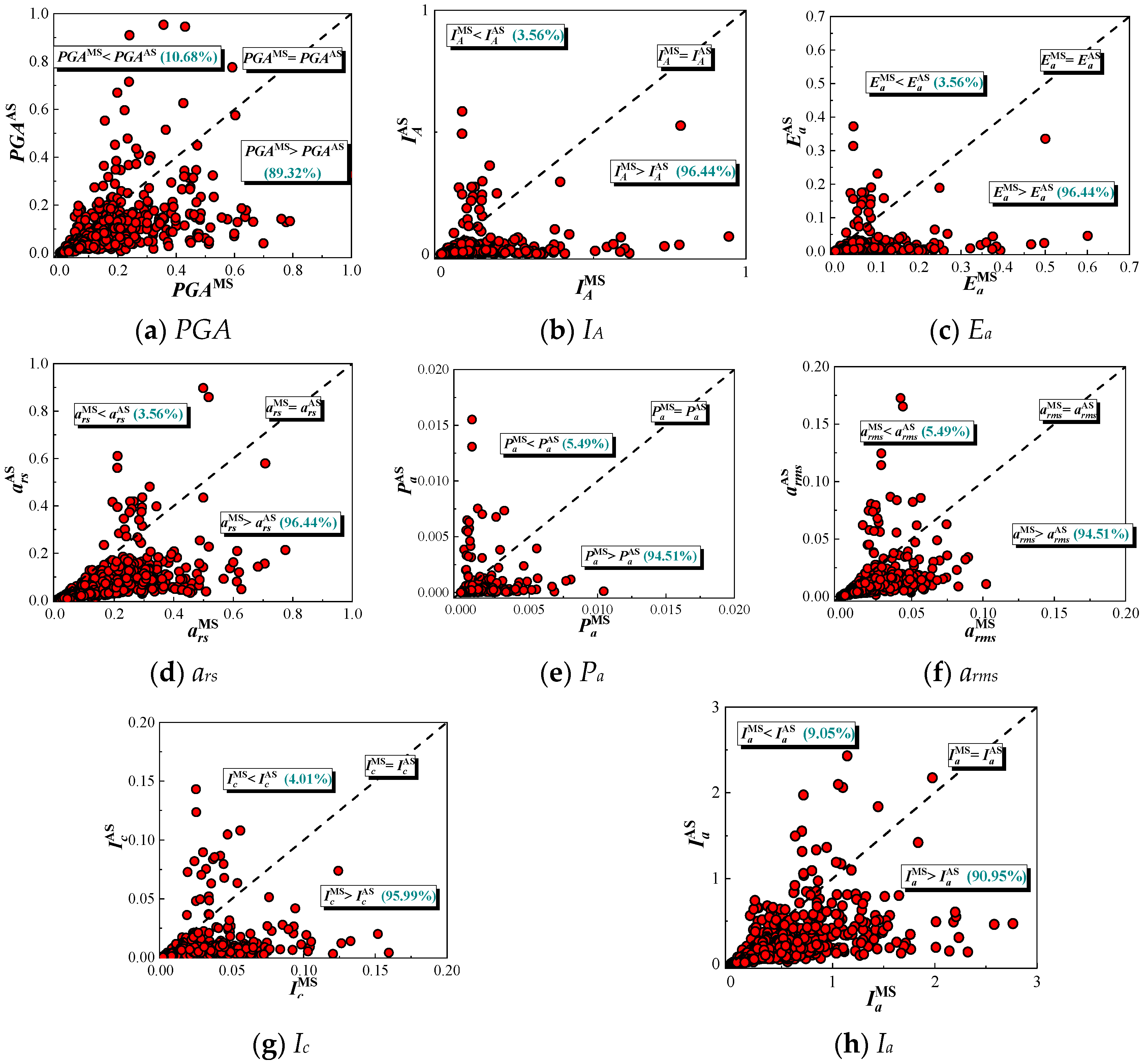
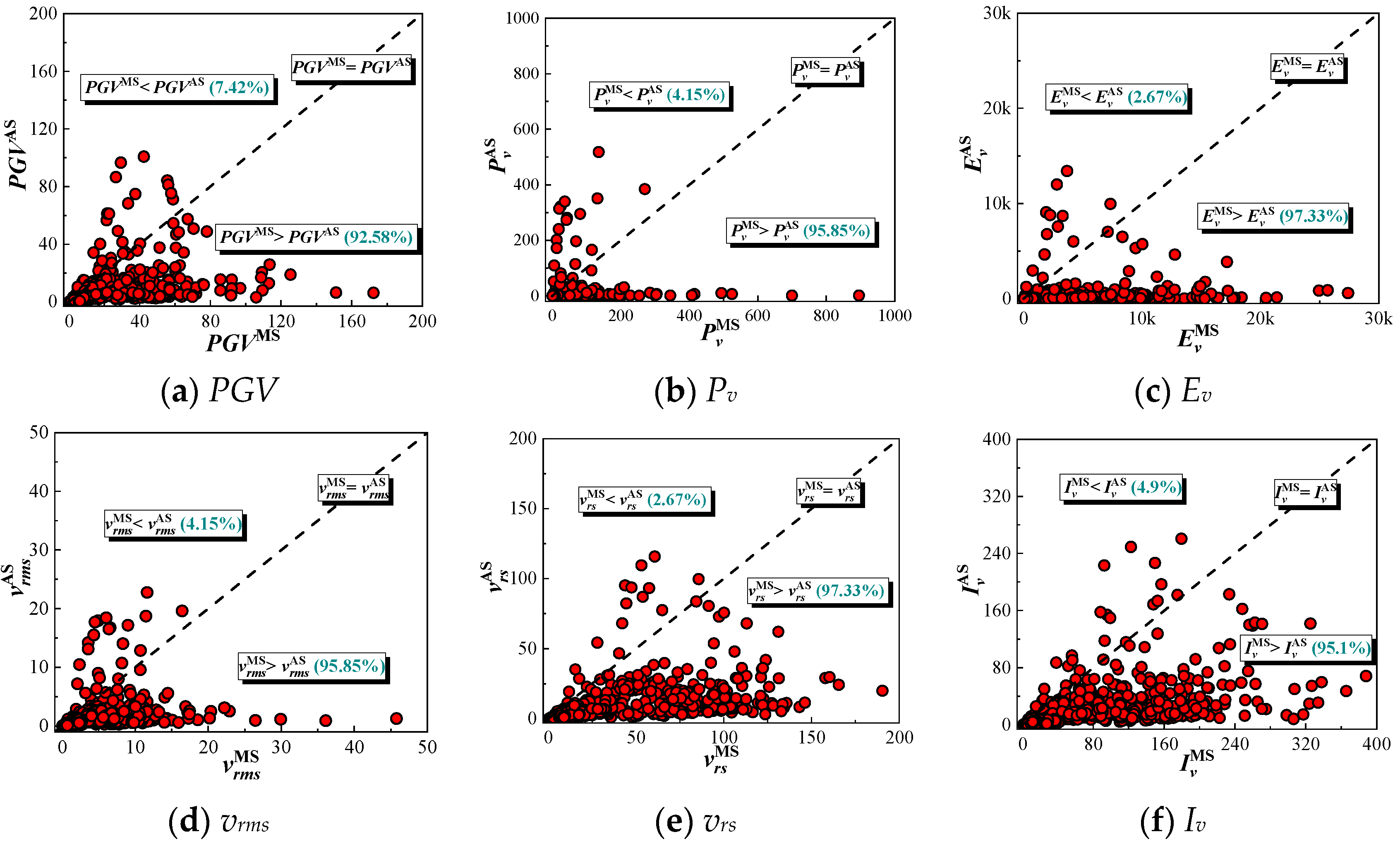
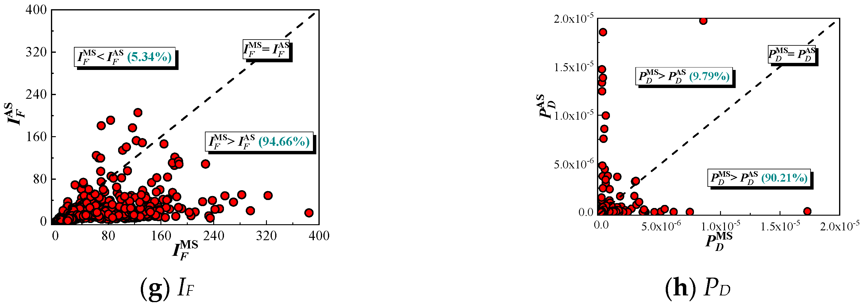
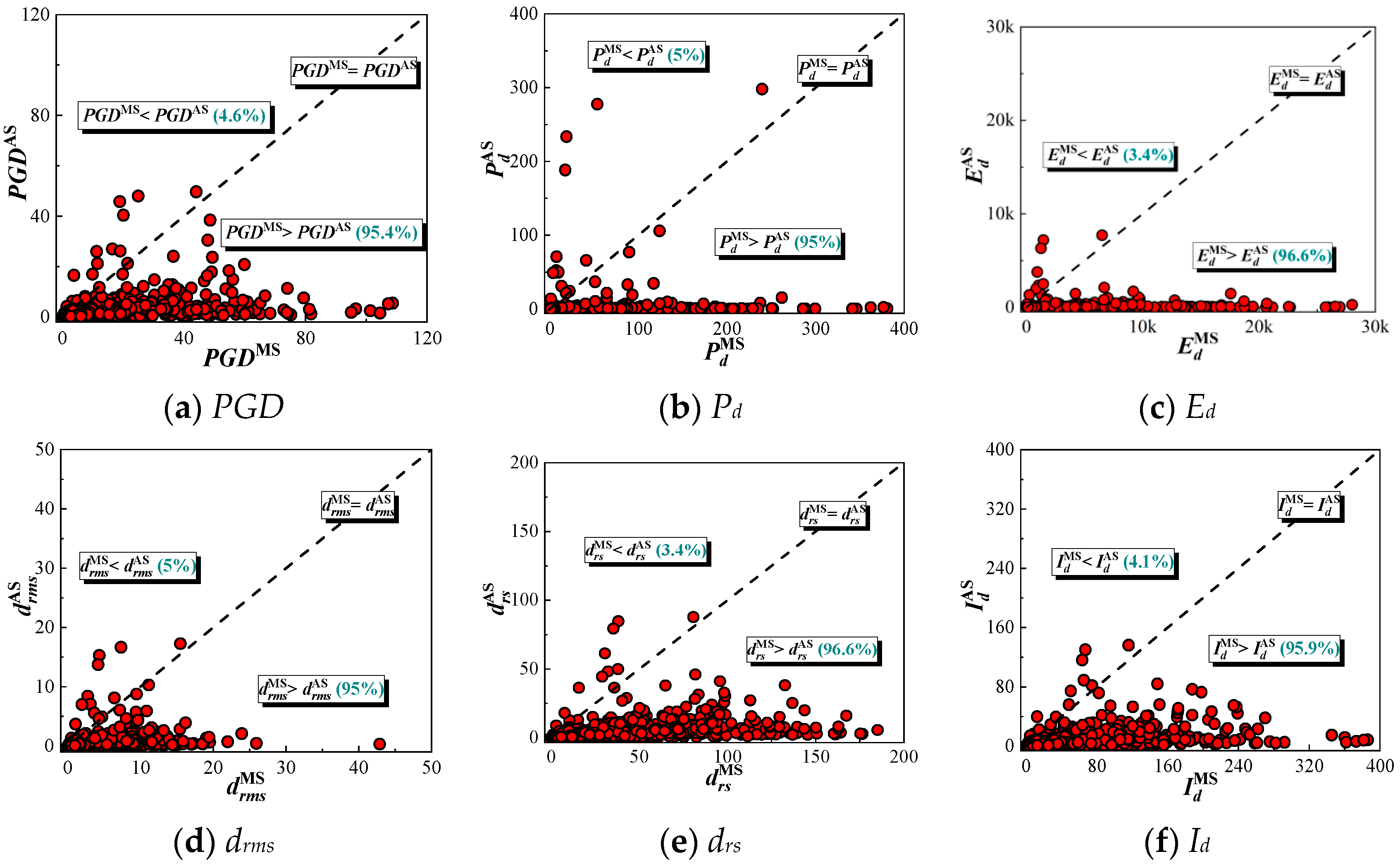
In this study, four categories of IMs were used to represent MS–AS sequences based on 22 classic IMs. They are PGA [46], IA [47], Pa [48], Ea [49], arms [50], ars [51], Ic [44], Ia [52], PGV [46], Pv [48], PD [53], Ev [49], vrms [50], vrs [51], Iv [52], IF [54], PGD [46], Pd [48], Ed [49], drms [50], drs [51], Id [52]. The 22 classic IMs have also been used in [38], which can be divided into three groups related to acceleration (see Figure 1), velocity (see Figure 2), and displacement (see Figure 3), respectively. It is noteworthy that the structure-specific IMs are not included in this study since they are commonly related to the structural fundamental period that would be elongated due to the MS-induced damage. In other words, two different structural periods are needed to define a structure-specific IM for the MS and the following AS. Thus, this study only adopts IMs associated with the basic properties of ground motions.
The considered four MS–AS IM categories include the mainshock IM, i.e., IMMS, and aftershock IM, i.e., IMAS, which are taken as the important intensity indicators for predicting the damage potential of MS–AS sequences according to Elenas et al. [42] and Kavvadias et al. [43], respectively. Besides IMMS and IMAS, two new types of IMs for MS–AS sequences were proposed herein, which are briefly represented by IM1MS–AS and IM2MS–AS. Using the considered 22 classic IMs, IM1MS–AS is defined by taking the entire MS–AS sequence as one nominal time history of ground motion acceleration. In particular, the peak amplitude-related IMs, including PGA, PGV, and PGD, are used to determine IM1MS–AS by max (IMMS, IMAS). As for the other IMs related to ground motion duration, they are used to define IM1MS–AS using the combined duration of the MS and the associated AS ground motions. As for IM2MS–AS, it is defined by the ratio of IMAS to IMMS, i.e., IM2MS–AS = IMAS/IMMS. It is clear that IM2MS–AS is a dimensionless and compound parameter by combing IMAS and IMMS together. Table 1, Table 2 and Table 3 provide the considered IMs related to acceleration, velocity, and displacement, respectively, and the corresponding definitions for MS–AS ground motions.
Figure 1, Figure 2 and Figure 3 show the obtained values of the 22 classic IMMS and IMAS by using the acceleration-, velocity-, and displacement-related IMs, respectively. It is found that most of the selected MS ground motions have larger intensities than the corresponding AS ground motions regardless of the IMs adopted, indicating significantly higher hazard caused by MSs compared to ASs. As observed, approximately over 90% (except only 89.32% of PGAMS values is greater than the corresponding PGAAS values, as shown in Figure 1a) of the considered MS ground motions show larger IMs than the corresponding AS ground motions. This result shows the larger damage potential of MSs than the corresponding ASs. Since the IA, Ea and ars have similar definition equations (see Table 1), their percentages corresponding to (Figure 1b), (Figure 1c), and (Figure 1d), respectively, are almost the same. Similar results can be also observed between Ev (Figure 2c) and vrs (Figure 2e) and that between Ed (Figure 3c) and drs (Figure 3e). Moreover, among the considered acceleration, velocity, and displacement IMs, the integral-formed IMs show slightly larger percentage with IMMS > IMAS than the other IMs.
3. Structural Damage under MS–AS Sequences
The damage index (DI) is used to simulate structural damage. In this study, four kinds of structural damage are considered, including the mainshock-induced damage for the initial system, i.e., DIMS, the AS-induced incremental damage for the mainshock-damaged system, i.e., DIAS|MS, the accumulative damage caused by MS–AS sequences, i.e., DI1MS–AS, and the ratio of between DIAS|MS and DIMS, i.e., DI2MS–AS = DIAS|MS/DIMS. In the following studies, DI1MS–AS is related to IMMS, IMAS, and IM1MS–AS, and DI2MS–AS is related to IM2MS–AS.
To determine DI1MS–AS and DI2MS–AS, the structural damage index proposed by Park and Ang [44] is adopted herein. The Park–Ang damage index is a linear combination of maximum deformation response and hysteretic energy dissipation. Therefore, it increases monotonically so that it is beneficial to quantify the accumulative damage caused by MS–AS sequences [15]. The Park–Ang damage index has been modified by Kunnath et al. [45], and the modified damage index, DI, is expressed by
where uy and uu are the yielding and ultimate displacements of a specific SDOF system under monotonic loading, respectively; umax and EH are the maximum displacement and absorbed energy of the system under earthquake loading, respectively; and β is the energy consumption factor, which is taken as β = 0.15 herein following Zhai et al. [15].
4. SDOF Systems
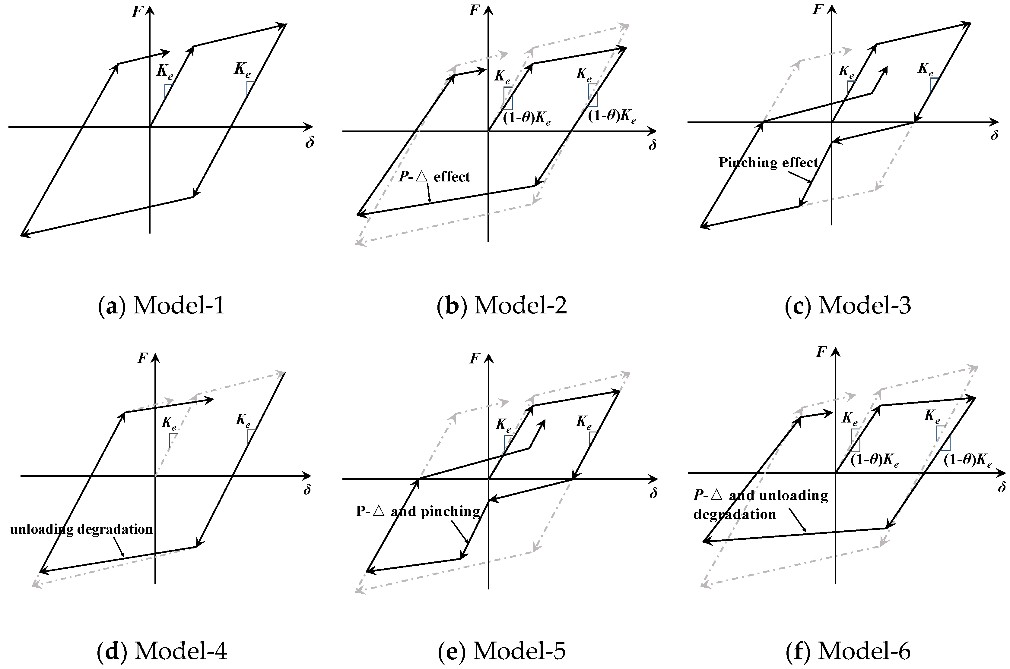
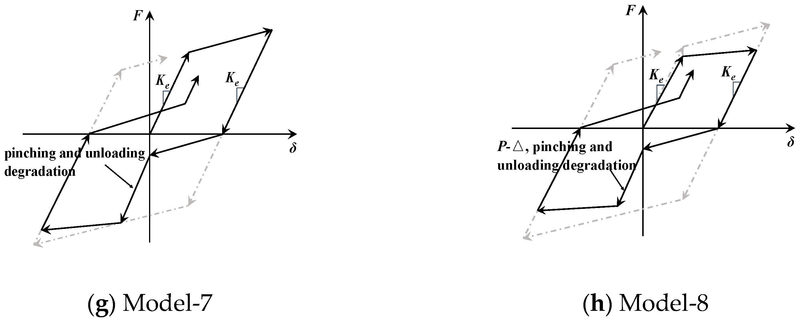
A total of eight different hysteretic models are considered herein to simulate the nonlinear behavior of SDOF systems under MS–AS sequences. Similar SDOF model assumptions and considerations have been used in [41]. Figure 4 shows the hysteretic rules of the considered models, where the force and displacement are both normalized by the yield force and yield displacement, respectively. A polygonal type of hysteretic model is adopted in this study for illustration. Compared to the smooth type of hysteretic models (e.g., Bouc–Wen models [55,56,57,58], which have the advantage of using a set of differential or algebraic equations), the polygonal type of hysteretic model requires less parameters, which can also include both strength and stiffness deterioration. The SDOF systems partly or totally w/wo considering P-Δ effect, pinching, and damage-induced deterioration are used to account for the varying hysteretic behaviors of the SDOF system. Table 4 provides the considered eight SDOF models, where Delta is the parameter controlling the P-Δ effect; PinchX and PinchY are the pinching factors for strain (or deformation) and stress (or force) during reloading, respectively; and Damage1 and Damage2 denote the damage due to ductility and energy, respectively, which are used to account for the deterioration due to damage.
Among the considered models, the basic model, which is numbered as Model-1, is an elastic-plastic-with-hardening model (see Figure 4a). Based on the basic model, three important factors, including the P-Δ effect, pinching effect, and unloading degradation, are partly or totally incorporated in Models 2–8 to reflect more complex nonlinear behaviors of structures under seismic loading. In particular, Models 2–4 represent the bilinear hysteretic models by individually considering the P-Δ effect, pinching effect, and unloading degradation, respectively (see Figure 4b–d). For Models 5–7, two of the above-stated influence factors are accounted for in the hysteretic behavior, as shown in Figure 4e–g, respectively. Besides, Model-8 has the most complex hysteretic behavior since it collectively incorporates the P-Δ effect, pinching effect, and unloading degradation (see Figure 4h). It is noteworthy that the considered Models 2–8 are used for parametric study to examine the effect of hysteretic models of SDOF systems on the obtained results.
A total of 44 fundamental vibration periods ranging from 0.2 s to 6.0 s are considered for each SDOF system, consisting of 29 periods between 0.2 s and 3.0 s (with an increment of 0.1 s), and 15 periods between 3.2 s and 6.0 s (with an interval of 0.2 s). Four yield strength reduction factors, i.e., R = 2, 3, 4, and 5, are considered to account for the varying ductility levels of structures. Moreover, a constant damping coefficient ξ = 0.05 is utilized for all the considered SDOF systems according the past available studies, such as [15,21]. It is noteworthy that the analysis process of this paper is also suitable for the cases with other ξ values. However, the discussion on the effect of damping ratios is beyond this study and will be discussed in the future work. Consequently, a total of 1408 (8 hysteretic models × 44 vibration periods × 4 ductility levels) SDOF systems are used in subsequent calculations.
5. Correlation Analysis
5.1. Selection of MS–AS Sequences
A set of 662 real MS–AS earthquake sequences were selected from 13 earthquake events based on the NGA-West2 database (https://peer.berkeley.edu/research/nga-west-2) (Ancheta et al [58]). The NGA-West2 database has been used to develop the latest generation of ground motion prediction equations for shallow crustal earthquakes (e.g., Campbell and Bozorgni [59], Du et al. [32] The detailed information of the selected ground motion records and the related earthquake events can be found in Zhu et al. [60]. It is noteworthy that, among the aftershock sequences triggered by a specific mainshock, only aftershock record with the largest magnitude was adopted. Moreover, the selected mainshock and associated aftershock ground motions should be recorded at the same station.
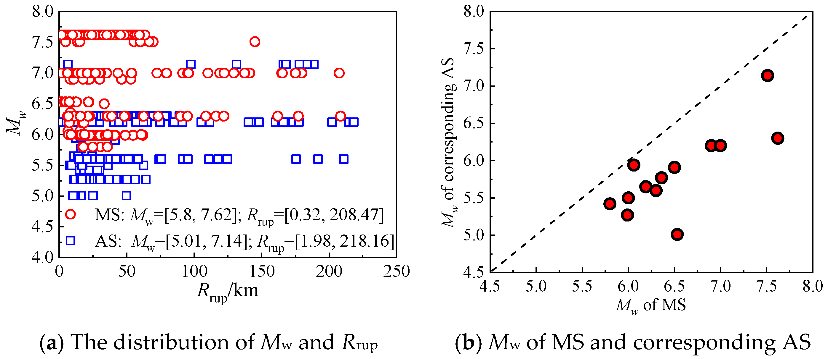
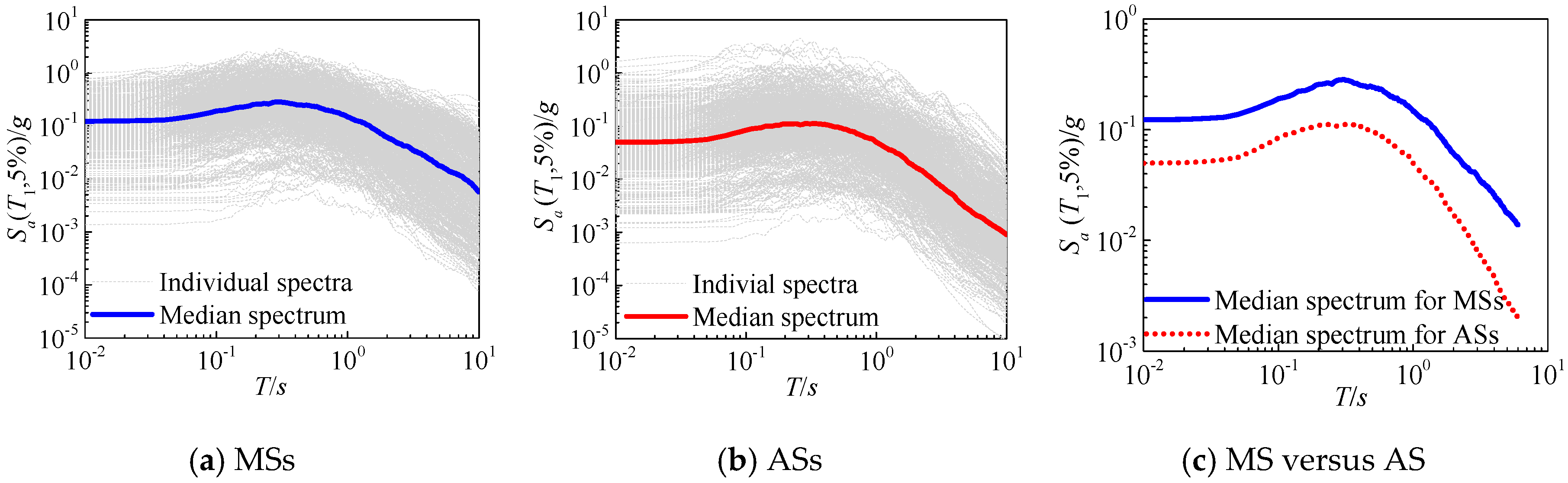
Figure 5 shows the distribution of moment magnitudes Mw and rupture distances Rrup for the selected ground motions of MSs and ASs. The magnitude of MSs ranges from Mw = 5.8 to Mw = 7.62, while the magnitude of the corresponding ASs ranges from Mw = 5.01 to Mw = 7.14. As for rupture distances, the range of Rrup for MSs is between 0.32 km and 208.47 km and that for ASs is between 1.98 km and 218.16 km, respectively. As seen from Figure 5b, the Mw values of MSs are always larger than that of AS. This is compatible with the Bath’s rule [61]. Figure 6 compares the elastic response spectra for the selected ground motions of MSs and ASs. It is found that the median response spectrum of MS ground motions is significantly larger than that of AS ground motions, which is expected due to the greater shaking intensities of MSs than ASs.
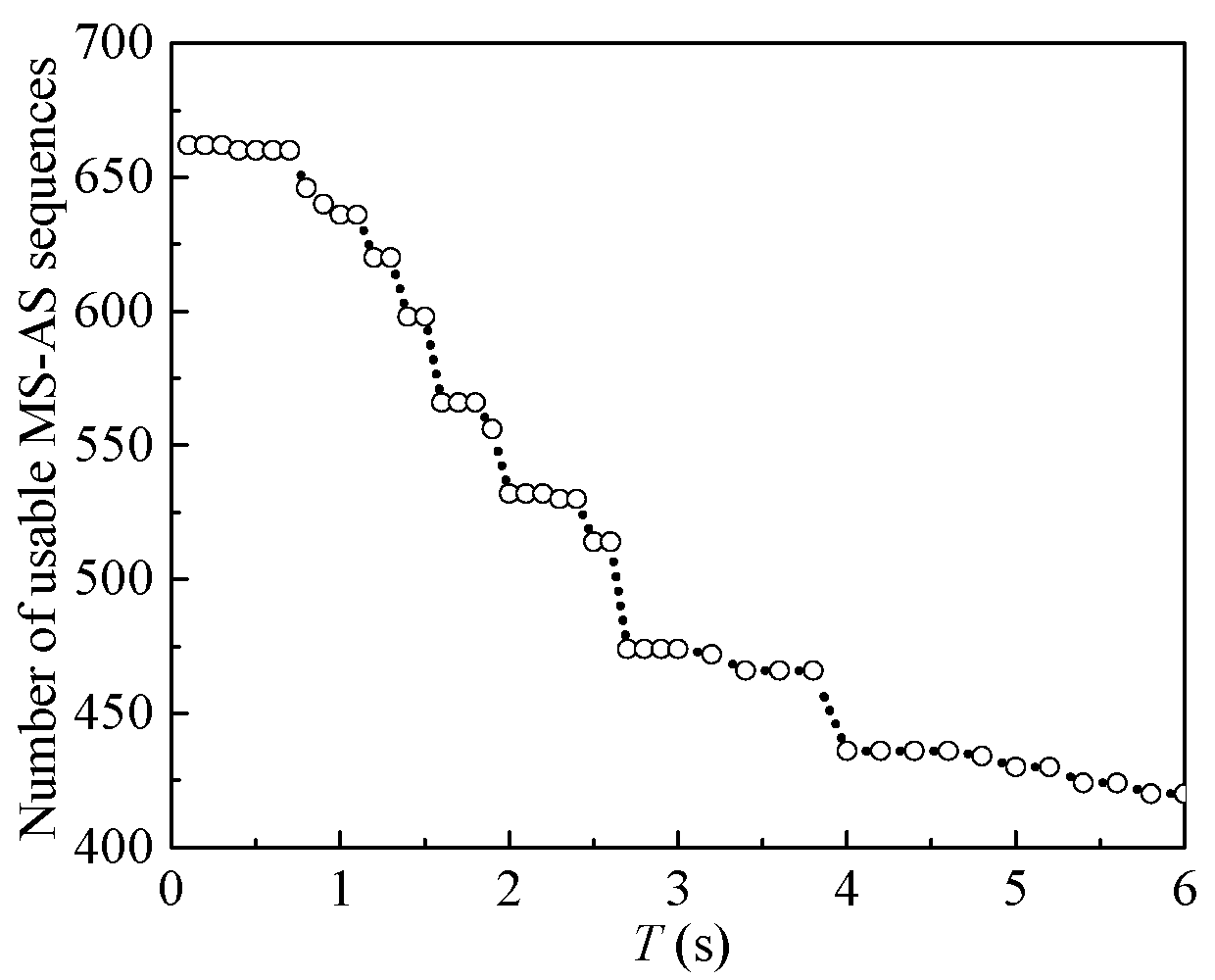
For a given ground motion recorder, it could only detect seismic signals in a certain range of frequency due to its settings. This makes the recorded ground motions have a specific lowest usage frequency, i.e., flow. Therefore, for dynamic analysis, a ground motion can only be used for nonlinear SDOF systems with their vibration periods no larger than T = 1/flow. As for a specific MS–AS sequence, the flow values for the MS and AS ground motions are probably different. For simplicity, the representative flow value for a MS–AS sequence is taken as max (flowMS, flowAS), where flowMS and flowAS are the flow values for the MS and AS ground motions, respectively. In this study, the highest structural period considered for the nonlinear SDOF systems is 6.0 s, and thus, the usable flow values of the selected MS–AS sequences should be no less than 0.166 Hz. Figure 7 shows the number of usable earthquake sequences at different periods with the consideration of flow requirement, where the number of usable sequences decreases with increasing periods of SDOF systems.
5.2. Correlation Coefficient
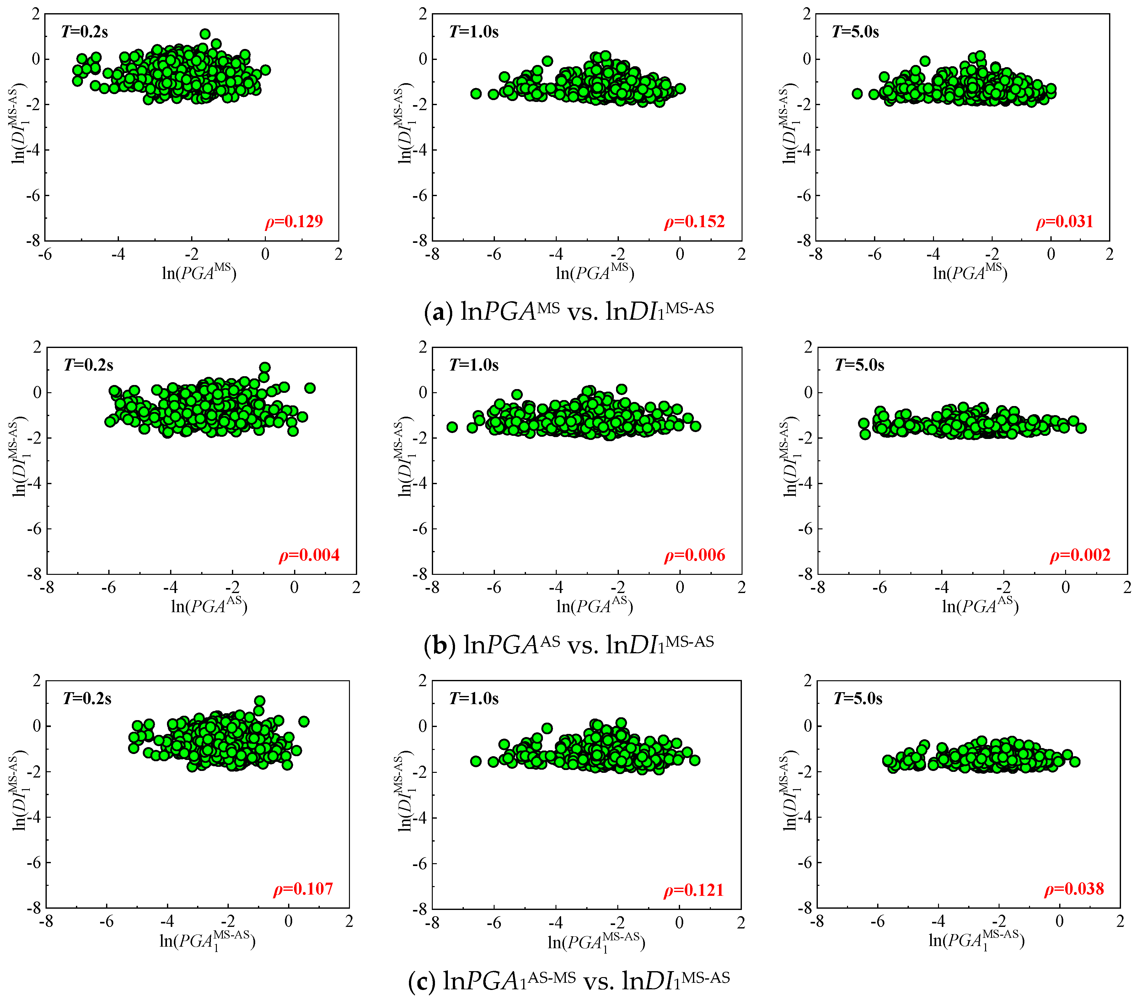
The Pearson correlation coefficient ρ is calculated for four IM-DI pairs in the logarithm space, including IMMS vs. DI1MS–AS, IMAS vs. DI1MS–AS, IM1MS–AS vs. DI1MS–AS, and IM2MS–AS vs. DI2MS–AS, respectively. The basic system with R = 2 at T = 0.2 s, 1.0 s, and 5.0 s are taken herein for illustration to represent the structure with short (acceleration-sensitive), medium (velocity-sensitive), and long (displacement-sensitive) vibration periods, respectively (Riddell [38]).
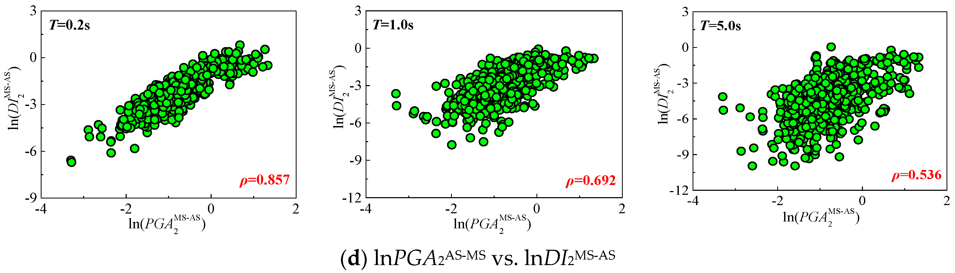
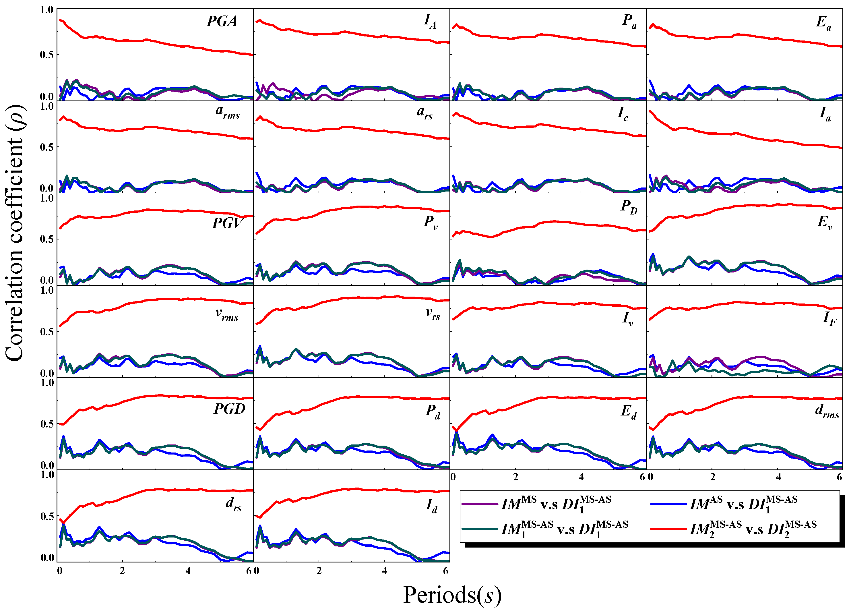
Figure 8 shows the scatters in terms of lnPGAMS vs. lnDI1MS–AS, lnPGAAS vs. lnDI1MS–AS, lnPGA1MS–AS vs. lnDI1MS–AS, and lnPGA2MS–AS vs. lnDI2MS–AS. It is clear that the correlation between the MS (or AS) intensity alone (i.e., PGAMS or PGAAS) and the structural cumulative damage (i.e., DI1MS–AS) is insignificant with the ρ values less than 0.3. Moreover, there is no clear improvement in the correlation between lnPGA1MS–AS and lnDI1MS–AS in which the entire earthquake sequence is regarded as one nominal ground motion. Yet, PGA2MS–AS shows a much stronger interdependence with DI2MS–AS, with correlation coefficients exceeding 0.5. Besides PGA, similar observation can also be obtained from the other IM-related data, which are summarized in Figure 9. As observed, the correlations between lnIM2MS–AS and lnDI2MS–AS for different considered IMs are always much larger than those of the other pairs (e.g., between lnIMMS and lnIM1MS–AS). These results confirm that IM2MS–AS performs much better than the other three types of IMs, i.e., IMM, IMAS, and IM1MS–AS, for the prediction of the damage potential of earthquake sequences.
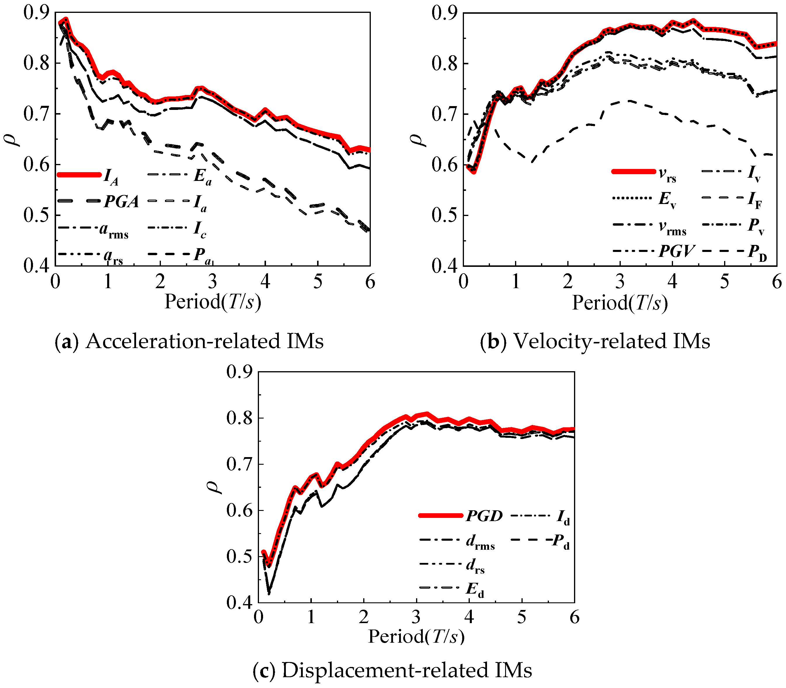
Figure 10 shows the correlations associated with the considered classic IMs between IM2MS–AS and DI2MS–AS. Among the acceleration-related IMs, IA is the most optimal one to generate IM2MS–AS since IA,2MS–AS has higher correlation with DI2MS–AS than Ea,2MS–AS, PGAMS–AS, Ia,2MS–AS, arms,2MS–AS, Ic,2MS–AS, ars,2MS–AS, and Pa,2MS–AS. As for the velocity-related and displacement-related IM groups, the corresponding optimal IMs are vrs and PGD, respectively.
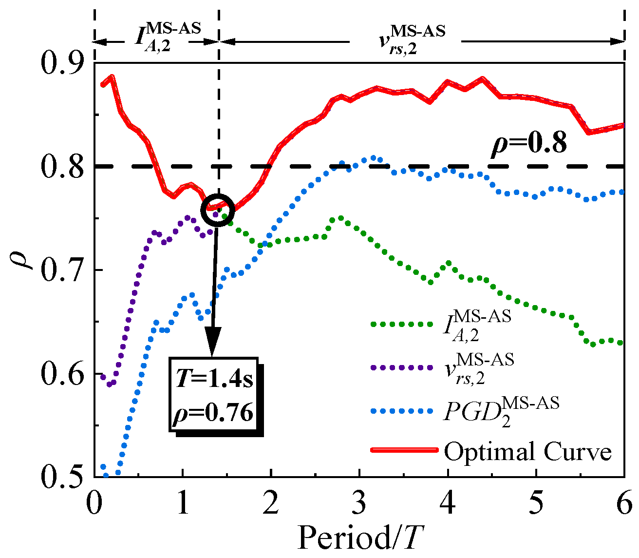
According to the results of Figure 10, IA, vrs and PGD are found as the optimal IMs to formulate IM2MS–AS in the acceleration-, velocity-, and displacement-based IM group, respectively. Then the ρ values between the three pairs, including IA,2MS–AS vs. DI2MS–AS, vrs,2MS–AS vs. DI2MS–AS, and PGD2MS–AS vs. DI2MS–AS, are plotted together at the entire period range, as shown in Figure 11. It is noteworthy that only the results related to the basic SDOF model (i.e., Model-1) are used. It is clear that there is no single IM exhibiting the best correlation throughout the entire period range, and thus, a transition period (i.e., Tc) exists. In fact, before and after Tc, IA and vrs are the most optimal IMs (with the highest correlation to DI2MS–AS) to formulate IM2MS–AS, respectively.
6. Effect of Hysteretic Models
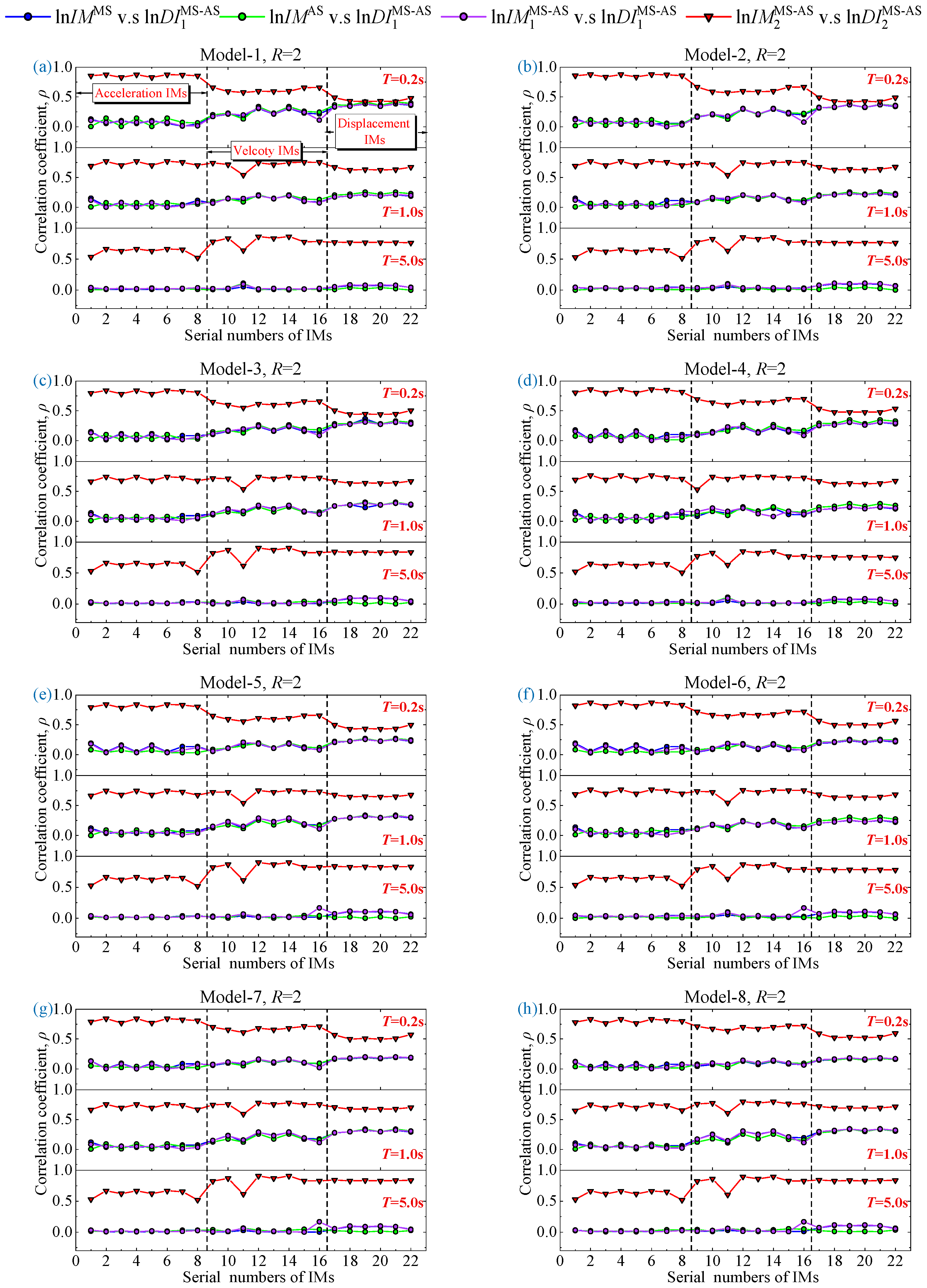
Two aspects of investigations are conducted on the effect of hysteretic models, including hysteretic model types and R levels. Figure 12 shows the calculated ρ values between the concerned four IM-DI pairs, including lnIMMS vs. lnDI1MS–AS, lnIMAS vs. lnDI1MS–AS, lnIM1MS–AS vs. lnDI1MS–AS, and lnIM2MS–AS vs. lnDI2MS–AS, using all the considered eight types of models with a constant R value of 2. As seen from this figure, the correlation between lnIM2MS–AS and lnDI2MS–AS is significantly higher than those of the other three IM-DI pairs regardless of the hysteretic model types. Among the acceleration-, velocity-, and displacement-related IMs, IA, vrs, and PGD are the most optimal IMs to formulate IM2MS–AS, respectively, due to the associated high correlation with DI2MS–AS. The observations stated above are consistent with those obtained in Figure 9. Moreover, varying hysteretic models does not cause significant differences in the obtained ρ values. Therefore, the effect of hysteretic model types on the obtained correlation results is limited and has no significant effect over the response for the current purposes.
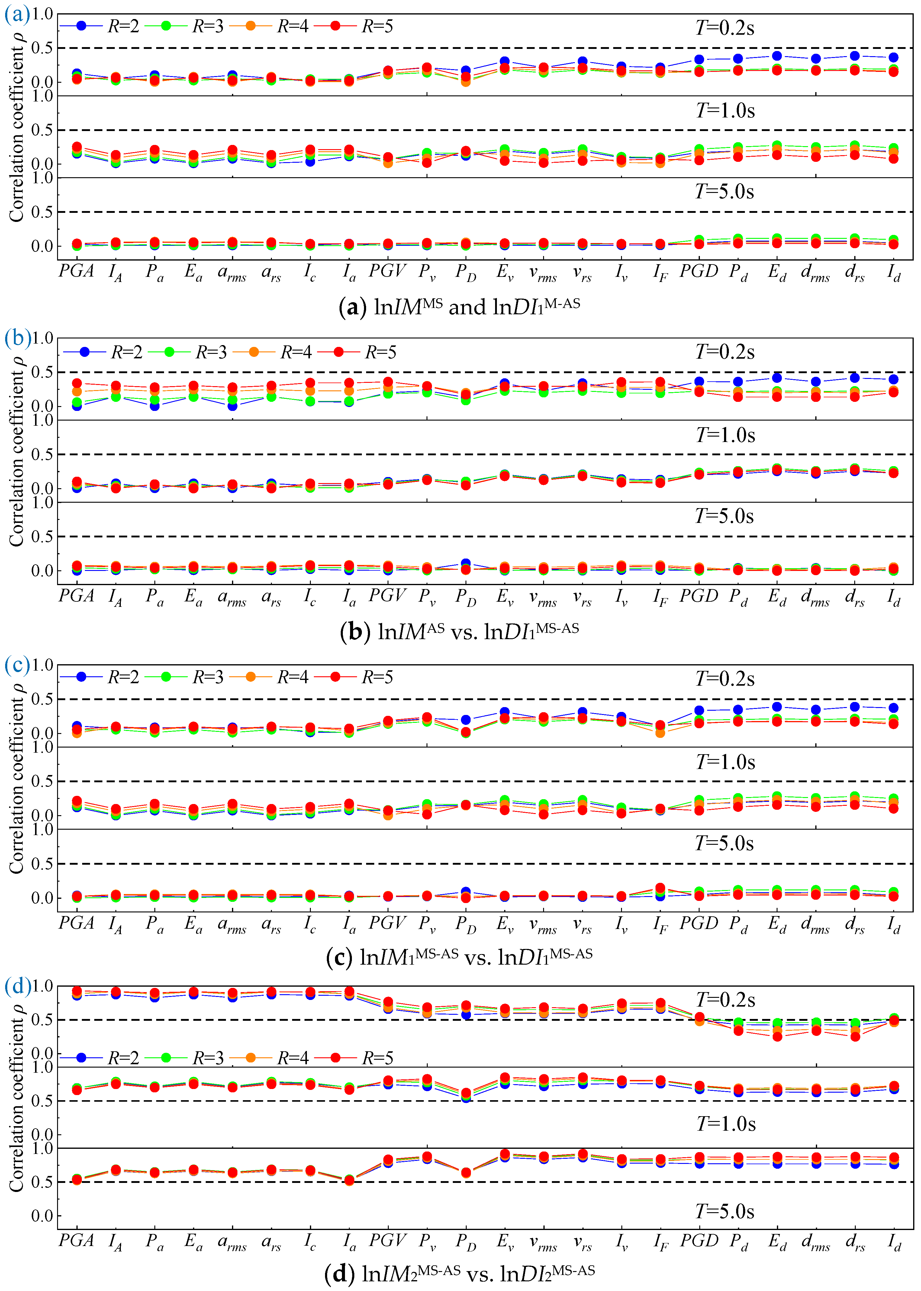
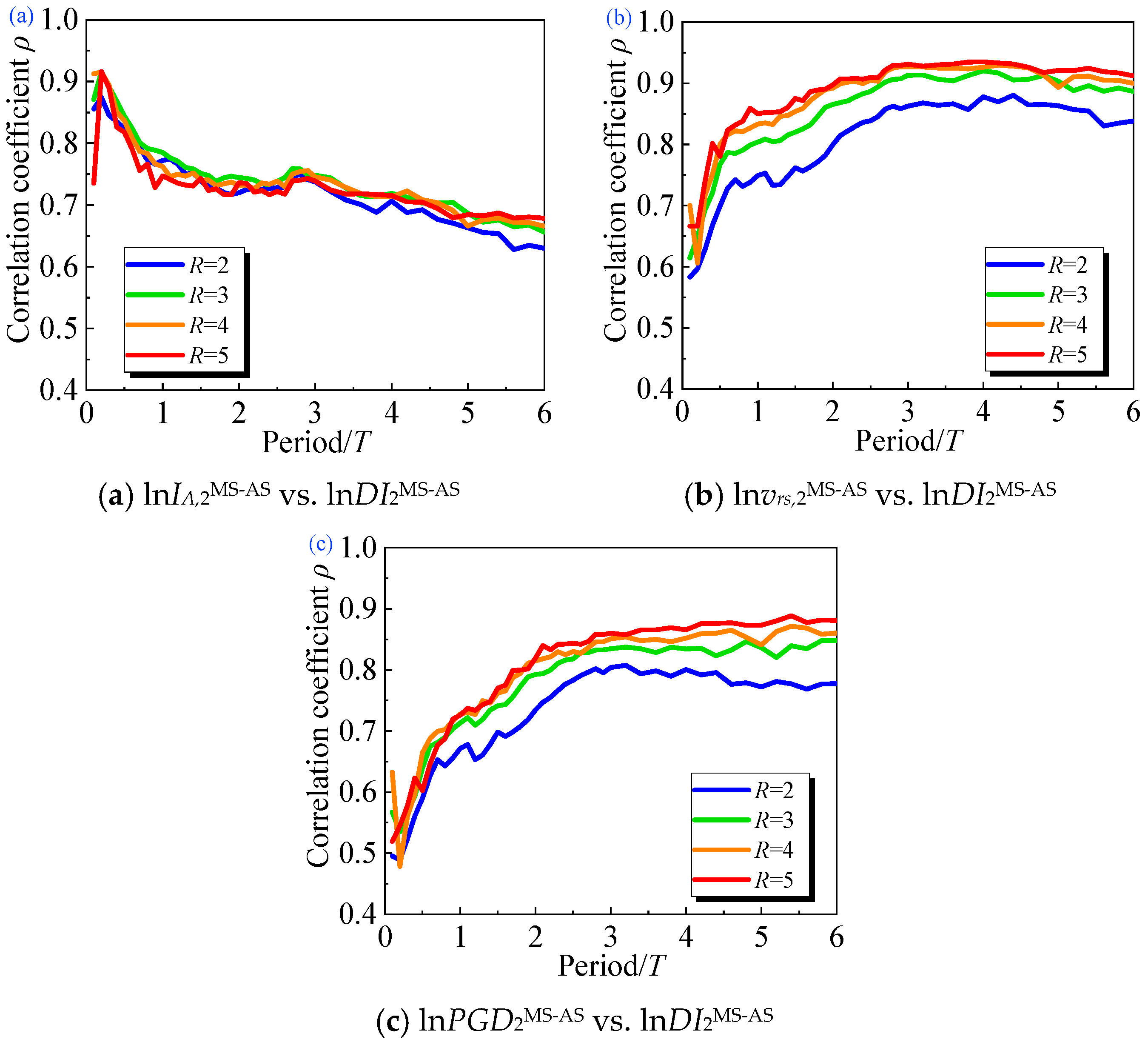
To examine the effect of strength reduction ratio, the systems simulated by the basic model with varying R values, i.e., R = 2~5, are adopted for illustration. Figure 13 compares the calculated ρ values between lnIMMS vs. lnDI1MS–AS, lnIMAS vs. lnDI1MS–AS, lnIM1MS–AS vs. lnDI1MS–AS, and lnIM2MS–AS vs. lnDI2MS–AS. It is clear that varying R values does not change the observations obtained in Figure 10 and Figure 11, including: (1) lnIM2MS–AS shows better performance than IMMS, IMAS, and IM1MS–AS due to its higher correlation with DI2MS–AS; and (2) IA, vrs, and PGD are the most optimal IMs to formulate IM2MS–AS among the acceleration-related, velocity-related and displacement-related IMs, respectively. Figure 14 illustrates the effect of changing R on the ρ values between IA,2MS–AS and DI2MS–AS, vrs,2MS–AS and DI2MS–AS, and PGD2MS–AS and DI2MS–AS at the entire period range. As observed, the change of R values yields a slightly larger difference on the ρ values than that of varying hysteretic models, especially for the two IM-DI pairs in terms of vrs,2MS–AS and DI2MS–AS, and PGD2MS–AS and DI2MS–AS. This is because a system with larger R value is easier to suffer nonlinear behavior under a MS excitation, leading to a more complex effect of the AS on the structural damage.
7. Empirical Prediction Equations
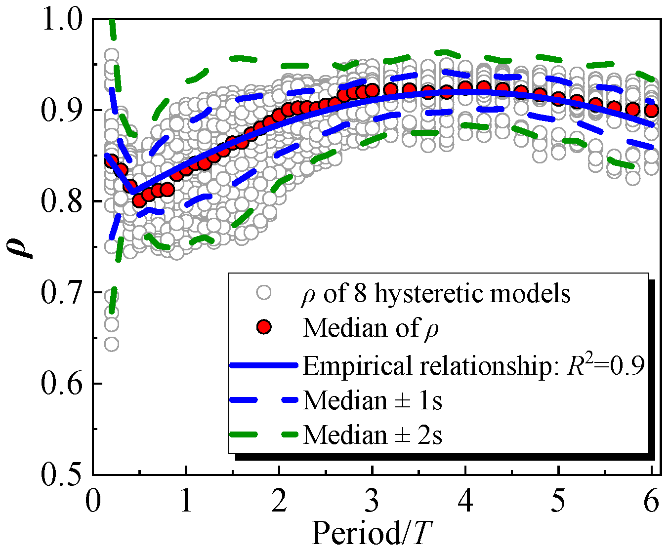
In this section, empirical equations are developed to predict the correlation coefficients, ρ, between the most optimal IM2MS–AS and the resulting DI2MS–AS. As seen from Figure 11, IA,2MS–AS and vrs,2MS–AS are separately the most optimal IM to formulate IM2MS–AS before and after the transition period Tc. This conclusion is verified with considering different hysteretic models and varying R levels in this section. Therefore, a step-wise relationship is feasible to represent the relationship between ρ and T. Figure 15 collects the calculated ρ values between the most optimal IM2MS–AS and DI2MS–AS corresponding to different hysteretic models with varying R values. From a viewpoint of median prediction, the median ρ values, i.e., ρ50%, at different T values are obtained by statistics; a stepwise equation consisting of a linear and a nonlinear section is regressed by Equation (2). It is clear that Equation (2) can appropriately fit the calculated ρ50% values with a coefficient of determination as R2 = 0.9.
where the transition period Tc is taken as 0.45 s. When T ≤ Tc, IA is recommended as the best candidate to formulate IA,2MS–AS = IAAS/IAMS with the corresponding correlation with DI2MS–AS approximated as ρ50% = −0.143 × T + 0.87. For the case of T < Tc < 6.0 s, vrs,2MS–AS = vrsAS/vrsMS is taken as the best IM for MS–AS sequences, whose median correlation with DI2MS–AS can be evaluated as ρ50% = 0.92 × exp{−[(T − 4)/10]2}. Based on Equation (2), the predicted correlation ρ50% is generally higher than 0.8, showing a significant interdependence between IA,2MS–AS (or vrs,2MS–AS) and DI2MS–AS. This result provides a basis that it is feasible to develop a linear relationship between IA,2MS–AS (or vrs,2MS–AS) and DI2MS–AS in logarithm space. This log-linear relationship is valuable for the quick assessment of structural damage caused by MS–AS sequences.
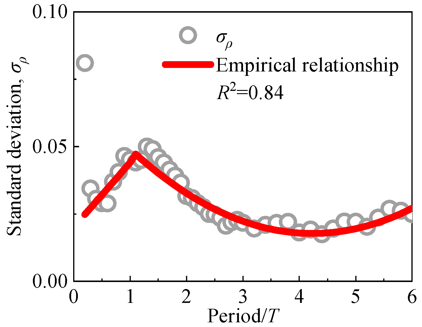
The variability of ρ in terms of the standard deviation σρ is further calculated based on the obtained ρ values. Figure 16 shows the σρ values along with the period. It is clear that a stepwise type equation is suitable to fit the σρ values. Then the stepwise function shown in Equation (3) is developed, which shows an acceptable goodness-of-fitting with a value of R2 equal to 0.84.
8. Discussions
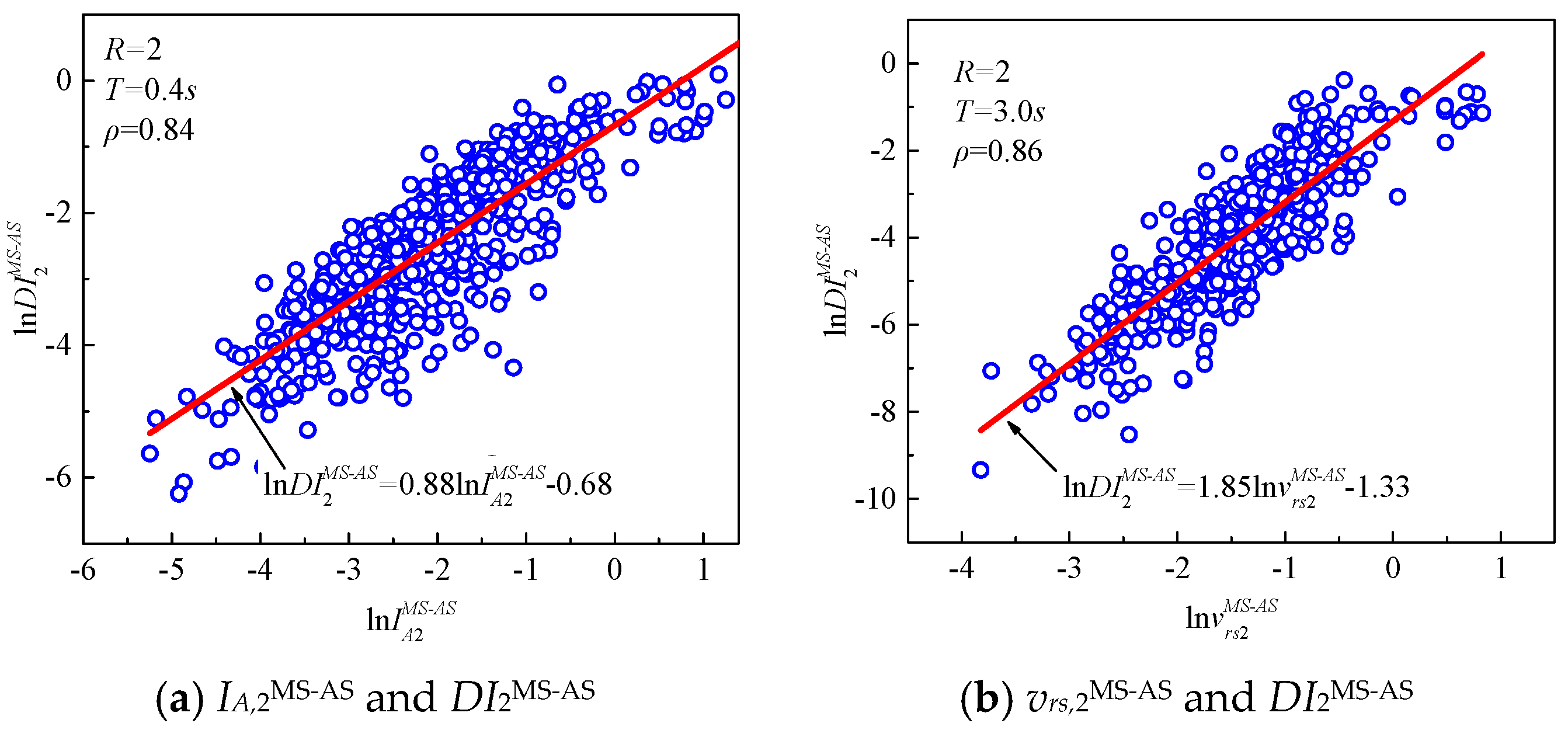
In this study, a new type of IM for MS–AS sequences, i.e., IM2MS–AS = IMAS/IMMS, is verified to be an desirable IM to predict MS–AS damage potential due to its high correlation with DI2MS–AS = DIAS|MS/DIMS. Based on this observation, reliable log-linear relationships can be established between IM2MS–AS and DI2MS–AS to predict the structural damage due to MS–AS sequences. Take the cases of T = 0.4 s and T = 3.0 s as examples; both periods are selected according to Equation (2) in the ranges of T ≤ Tc and T < Tc < 6.0 s, respectively. According to the results of Section 5 and Section 6, IA,2MS–AS and vrs,2MS–AS are proven to be the optimal IMs, respectively. The linear regressions between IA,2MS–AS and DI2MS–AS and between vrs,2MS–AS and DI2MS–AS are also provided at log-log axis in Figure 17.
It is clear that clear linear relationships have been developed in these two figures. Based on the developed log-linear relationships, once the IMs of the mainshock and the following aftershock are determined, the damage ratio DI1MS–AS can be predicted directly. If the initial damage of structures due to mainshock (i.e., DIMS) has been estimated, the aftershock-induced damage increment (i.e., DIAS|MS) and the accumulative damages (i.e., DI1MS–AS) due to the MS–AS sequence can be further calculated. Besides, a reliable log-linear relationship between IM2MS–AS and DI2MS–AS is also useful for fragility assessment under MS–AS sequences since it commonly assumes a log-linear relationship between earthquake IMs and engineering demand parameters (EDPs). To sum up, there are three folds of applications of the developed log-linear relationship between IM2MS–AS and DI2MS–AS, as: (1) to predict DI2MS–AS given IM2MS–AS; (2) to predict DI1MS–AS and DIAS|MS given IM2MS–AS and DIMS; and (3) to represent the relationship between IM and EDP for fragility assessment under MS–AS sequences.
9. Conclusions
The damage potential for MS–AS sequences was comprehensively conducted by examining the correlation between the intensities of MS–AS sequences and the corresponding structural damage. The following general conclusions have been drawn:
- (1)
- The correlations between IMMS and DI1MS–AS, IMAS and DI1MS–AS, IM1MS–AS and DI1MS–AS, and IM2MS–AS and DI2MS–AS were examined in the logarithm space for the SDOF systems with varying periods. The results show that the IM-DI pair in terms of IM2MS–AS and DI2MS–AS has the highest correlation among the considered four IM-DI pairs. In other words, the proposed IM, which is defined as IMAS/IMMS, has a better capability to predict damage potential caused by earthquake sequences in comparison with IMMS, IMAS, and IM1MS–AS.
- (2)
- A total of 22 classic IMs were considered as the candidates to define the intensities of MS–AS sequences. Amongst these IMs, IA, vrs, and PGD are the most optimal ones to formulate IM2MS–AS for the acceleration-related, velocity-related, and displacement-related IM groups, respectively, due to the high correlations with DI2MS–AS. There is no single IM to best formulate IM2MS–AS in the entire structural period range. IA,2MS–AS and vrs,2MS–AS are the best IMs before and after a transition period Tc, separately.
- (3)
- A comprehensive parametric study was conducted by considering various types of hysteretic models and different yield reduction factors. The results show that the effects of varying hysteretic models and yielding reduction factors are limited on the correlation between IM2MS–AS and DI2MS–AS. This result reveals that the obtained conclusion in this study is in a general prospect.
- (4)
- A step-wise equation consisting of linear and nonlinear parts was regressed as the median prediction of ρ between the best IM2MS–AS and the caused DI2MS–AS. Moreover, through regression analysis, another step-wise function was developed to denote the standard deviation of the ρ values along with T. The empirical equations can fit the obtained data reasonably well, providing an opportunity for the further studies to conduct a quick prediction of damage potential for a specific MS–AS earthquake sequence.
Author Contributions
Conceptualization, Z.Z. and X.Y.; methodology, X.Y.; validation, Z.Z.; formal analysis, Z.Z. and X.Y.; data curation, Z.Z.; writing—original draft preparation, Z.Z.; writing—review and editing, X.Y.; supervision, X.Y. and D.L.; funding acquisition, X.Y. and D.L. All authors have read and agreed to the published version of the manuscript.
Funding
This research was funded by the Scientific Research Fund of the Institute of Engineering Mechanics, China Earthquake Administration (grant no. 2018D08), the National Natural Science Foundation of China (grant no. 51778198; 51678209).
Conflicts of Interest
The authors declare no conflict of interest.
Abbreviations
| Descriptions | Abbreviation |
| Intensity measure | IM |
| Engineering demand parameter | EDP |
| Damage index | DI |
| Mainshock | MS |
| Aftershock | AS |
| Mainshock–aftershock sequences | MS–AS sequences |
| Yield strength reduction factor | R |
| Peak ground acceleration | PGA |
| Arias intensity | IA |
| Mean-square acceleration | Pa |
| Square acceleration | Ea |
| Root-mean square acceleration | arms |
| Root-square acceleration | ars |
| Characteristic intensity | Ic |
| Riddell acceleration intensity | Ia |
| Peak ground velocity | PGV |
| Mean-square velocity | Pv |
| Potential destructiveness | PD |
| Square velocity | Ev |
| Root-mean square velocity | vrms |
| Root-square velocity | vrs |
| Riddell velocity intensity | Iv |
| Fajfar intensity | IF |
| Peak ground displacement | PGD |
| Mean-square displacement | Pd |
| Square displacement | Ed |
| Root-mean square displacement | drms |
| Root-square displacement | drs |
| Riddell displacement intensity | Id |
| Correlation coefficient | ρ |
References
- Kao, H. The Chi-Chi Earthquake sequence: Active, out-of-sequence thrust faulting in Taiwan. Science 2000, 288, 2346–2349. [Google Scholar] [CrossRef] [PubMed] [Green Version]
- Huang, Y.; Wu, J.; Zhang, T.; Zhang, D. Relocation of the M8.0 Wenchuan earthquake and its aftershock sequence. Sci. China Ser. D Earth Sci. 2008, 51, 1703–1711. [Google Scholar] [CrossRef]
- Chian, S.C.; Pomonis, A.; Saito, K.; Fraser, S.; Goda, K.; Macabuag, J.; Offord, M.; Raby, A.; Sammonds, P. Post earthquake field investigation of the Mw9.0 Tōhoku earthquake of 11th March 2011. In Proceedings of the 15th World Conference on Earthquake Engineering, Lisbon, Portugal, 24–28 September 2012. [Google Scholar]
- Mahin, S.A. Effects of duration and aftershocks on inelastic design earthquakes. In Proceedings of the 7th world Conference on Earthquake Engineering, Istanbul, Turkey, 8–13 September 1980; Volume 5, pp. 677–680. [Google Scholar]
- Aschheim, M.; Black, E. Effects of prior earthquake damage on response of simple stiffness-degrading structures. Earthq. Spectra 1999, 15, 1–24. [Google Scholar] [CrossRef]
- Hatzigeorgiou, G.D.; Beskos, D.E. Inelastic displacement ratios for SDOF structures subjected to repeated earthquakes. Eng. Struct. 2009, 31, 2744–2755. [Google Scholar] [CrossRef]
- Zhai, C.H.; Wen, W.P.; Zhu, T.T.; Li, S.; Xie, L.L. Inelastic displacement ratios for design of structures with constant damage performance. Eng. Struct. 2013, 52, 53–63. [Google Scholar] [CrossRef]
- Amadio, C.; Fragiacomo, M.; Rajgelj, S. The effects of repeated earthquake ground motions on the non-linear response of SDOF systems. Earthq. Eng. Struct. Dyn. 2002, 32, 291–308. [Google Scholar] [CrossRef]
- Hatzigeorgiou, G.D. Ductility demand spectra for multiple near- and far-fault earthquakes. Soil Dyn. Earthq. Eng. 2010, 30, 170–183. [Google Scholar] [CrossRef]
- Hatzigeorgiou, G.D. Behavior factors for nonlinear structures subjected to multiple near-fault earthquakes. Comput. Struct. 2010, 88, 309–321. [Google Scholar] [CrossRef]
- Goda, K.; Taylor, C.A. Effects of aftershocks on peak ductility demand due to strong ground motion records from shallow crustal earthquakes. Earthq. Eng. Struct. Dyn. 2012, 41, 2311–2330. [Google Scholar] [CrossRef]
- Goda, K. Nonlinear response potential of mainshock-aftershock sequences from Japanese earthquakes. Bull. Seism. Soc. Am. 2012, 102, 2139–2156. [Google Scholar] [CrossRef]
- Yaghmaei-Sabegh, S.; Ruiz-García, J. Nonlinear response analysis of SDOF systems subjected to doublet earthquake ground motions: A case study on 2012 Varzaghan–Ahar events. Eng. Struct. 2016, 110, 281–292. [Google Scholar] [CrossRef]
- Zhai, C.; Ji, D.; Wen, W.; Lei, W.; Xie, L.; Gong, M. The inelastic input energy spectra for main shock–aftershock sequences. Earthq. Spectra 2016, 32, 2149–2166. [Google Scholar] [CrossRef]
- Zhai, C.H.; Wen, W.P.; Chen, Z.; Li, S.; Xie, L.L. Damage spectra for the mainshock–aftershock sequence-type ground motions. Soil Dyn. Earthq. Eng. 2013, 45, 1–12. [Google Scholar] [CrossRef]
- Yu, X.; Li, S.; Lü, D.-G.; Tao, J. Collapse capacity of inelastic single-degree-of-freedom systems subjected to mainshock-aftershock earthquake sequences. J. Earthq. Eng. 2020, 24, 803–826. [Google Scholar] [CrossRef]
- Ruiz-García, J.; Yaghmaei-Sabegh, S.; Bojórquez, E. Three-dimensional response of steel moment-resisting buildings under seismic sequences. Eng. Struct. 2018, 175, 399–414. [Google Scholar] [CrossRef]
- Ruiz-García, J.; Marín, M.V.; Teran-Gilmore, A. Effect of seismic sequences in reinforced concrete frame buildings located in soft-soil sites. Soil Dyn. Earthq. Eng. 2014, 63, 56–68. [Google Scholar] [CrossRef]
- Tesfamariam, S.; Goda, K.; Mondal, G. Seismic vulnerability of reinforced concrete frame with unreinforced masonry infill due to main shock–aftershock earthquake sequences. Earthq. Spectra 2015, 31, 1427–1449. [Google Scholar] [CrossRef]
- Liu, Y.; Yu, X.; MA, F. Impact of initial damage path and spectral shape on aftershock collapse fragility of RC frame. Earthq. Struct. 2018, 15, 529–540. [Google Scholar]
- Goda, K.; Salami, M.R. Inelastic seismic demand estimation of wood-frame houses subjected to mainshock-aftershock sequences. Bull. Earthq. Eng. 2014, 12, 855–874. [Google Scholar] [CrossRef]
- Yaghmaei-Sabegh, S.; Panjehbashi-Aghdam, P. Damage assessment of adjacent fixed- and isolated-base buildings under multiple ground motions. J. Earthq. Eng. 2018, 1–29. [Google Scholar] [CrossRef]
- Ghosh, J.; Padgett, J.E.; Sánchez-Silva, M. Seismic damage accumulation in highway bridges in earthquake-prone regions. Earthq. Spectra 2015, 31, 115–135. [Google Scholar] [CrossRef] [Green Version]
- Bertetto, A.M.; Masera, D.; Carpinteri, A. Acoustic emission monitoring of the turin cathedral bell tower: Foreshock and aftershock discrimination. Appl. Sci. 2020, 10, 3931. [Google Scholar] [CrossRef]
- Aloisio, A.; Antonacci, E.; Fragiacomo, M.; Alaggio, R. The recorded seismic response of the Santa Maria di collemaggio basilica to low-intensity earthquakes. Int. J. Arch. Heritage 2020, 1–19. [Google Scholar] [CrossRef]
- Akkar, S.; Ozen, O. Effect of peak ground velocity on deformation demands for SDOF systems. Earthq. Eng. Struct. Dyn. 2005, 34, 1551–1571. [Google Scholar] [CrossRef]
- Alvanitopoulos, P.F.; Andreadis, I.; Elenas, A. Interdependence between damage indices and ground motion parameters based on Hilbert–Huang transform. Meas. Sci. Technol. 2009, 21, 25101. [Google Scholar] [CrossRef]
- Elenas, A. Interdependency between seismic acceleration parameters and the behaviour of structures. Soil Dyn. Earthq. Eng. 1997, 16, 317–322. [Google Scholar] [CrossRef]
- Elenas, A. Correlation between seismic acceleration parameters and overall structural damage indices of buildings. Soil Dyn. Earthq. Eng. 2000, 20, 93–100. [Google Scholar] [CrossRef]
- Elenas, A.; Meskouris, K. Correlation study between seismic acceleration parameters and damage indices of structures. Eng. Struct. 2001, 23, 698–704. [Google Scholar] [CrossRef]
- Yakut, A.; Yılmaz, H. Correlation of deformation demands with ground motion intensity. J. Struct. Eng. 2008, 134, 1818–1828. [Google Scholar] [CrossRef]
- Du, W.; Yu, X.; Ning, C.L. Influence of earthquake duration on structural collapse assessment using hazard-consistent ground motions for shallow crustal earthquakes. Bull. Earthq. Eng. 2020, 18, 3005–3023. [Google Scholar] [CrossRef]
- Van Cao, V.; Ronagh, H.R. Correlation between parameters of pulse-type motions and damage of low-rise RC frames. Earthq. Struct. 2014, 7, 365–384. [Google Scholar] [CrossRef]
- Van Cao, V.; Ronagh, H.R. Correlation between seismic parameters of far-fault motions and damage indices of low-rise reinforced concrete frames. Soil Dyn. Earthq. Eng. 2014, 66, 102–112. [Google Scholar] [CrossRef]
- Kostinakis, K.; Athanatopoulou, A.; Morfidis, K. Correlation between ground motion intensity measures and seismic damage of 3D R/C buildings. Eng. Struct. 2015, 82, 151–167. [Google Scholar] [CrossRef]
- Lucchini, A.; Mollaioli, F.; Monti, G. Intensity measures for response prediction of a torsional building subjected to bi-directional earthquake ground motion. Bull. Earthq. Eng. 2011, 9, 1499–1518. [Google Scholar] [CrossRef]
- Mollaioli, F.; Lucchini, A.; Cheng, Y.; Monti, G. Intensity measures for the seismic response prediction of base-isolated buildings. Bull. Earthq. Eng. 2013, 11, 1841–1866. [Google Scholar] [CrossRef]
- Riddell, R. On ground motion intensity indices. Earthq. Spectra 2007, 23, 147–173. [Google Scholar] [CrossRef]
- Fontara, I.K.M.; Athanatopoulou, A.M.; Avramidis, I.E. Correlation between advanced structure-specific ground motion intensity measures and damage indices. In Proceedings of the 15th World Conference on Earthquake Engineering, Lisbon, Portugal, 24–28 September 2012. [Google Scholar]
- Ozmen, H.B.; Inel, M. Damage potential of earthquake records for RC building stock. Earthq. Struct. 2016, 10, 1315–1330. [Google Scholar] [CrossRef]
- Liu, T.T.; Yu, X.; Lü, D.G. An approach to develop compound intensity measures for prediction of damage potential of earthquake records using canonical correlation analysis. J. Earthq. Eng. 2018, 1–24. [Google Scholar] [CrossRef]
- Elenas, A.; Siouris, I.M.; Plexidas, A. A study on the interrelation of seismic intensity parameters and damage indices of structures under mainshock-aftershock seismic sequences. In Proceedings of the 16th World Conference on Earthquake Engineering, Santiago, MN, USA, 8–13 January 2017. [Google Scholar]
- Kavvadias, I.E.; Rovithis, P.Z.; Lazaros, K.V.; Elenas, A. Effect of the aftershock intensity characteristics on the seismic response of RC frame buildings. In Proceedings of the 16th European Conference on Earthquake Engineering, Thessaloniki, Greece, 18–21 June 2018. [Google Scholar]
- Park, Y.; Ang, A.H.; Wen, Y.K. Seismic damage analysis of reinforced concrete buildings. J. Struct. Eng. 1985, 111, 740–757. [Google Scholar] [CrossRef]
- Kunnath, S.K.; Reinhorn, A.M.; Park, Y.J. Analytical modeling of inelastic seismic response of R/C structures. J. Struct. Eng. 1990, 116, 996–1017. [Google Scholar] [CrossRef]
- Kramer, S. Performance-based design methodologies for geotechnical earthquake engineering. Bull. Earthq. Eng. 2013, 12, 1049–1070. [Google Scholar] [CrossRef]
- Arias, A. A measure of earthquake intensity. In Seismic Design of Nuclear Power Plants; Hansen, R., Ed.; MIT Press: Cambridge, MA, USA, 1970; pp. 438–483. [Google Scholar]
- Housner, G.W. Measures of severity of earthquake ground shaking. In Proceedings of the US National Conference on Earthquake Engineering, Earthquake Engineering Research Institute, Ann Arbor, MI, USA, 18–20 June 1975; pp. 25–33. [Google Scholar]
- Nau, J.M.; Hall, W.J. An Evaluation of Scaling Methods for Earthquake Response Spectra; Technical Report; Department of Civil Engineering, University of Illinois at Urbana: Champaign IL, USA, 1982. [Google Scholar]
- Housner, G.W.; Jennings, P.C. Generation of artificial earthquakes. Eng. Mech. 1964, 90, 113–152. [Google Scholar]
- Housner, G.W. Strong ground motion. In Recent Advances in Earthquake Engineering; Wiegel, R.L., Ed.; Prentive Hall Inc.: Englewood Cliffs, NJ, USA, 1970. [Google Scholar]
- Riddell, R.; García, J.E. Hysteretic energy spectrum and damage control. Earthq. Eng. Struct. Dyn. 2001, 30, 1791–1816. [Google Scholar] [CrossRef]
- Araya, R.; Saragoni, R. Capacidad De Los Movimientos Sísmicos De Producir Daño Estructural; Division of Structural Engineering; Department of Engineering, University of Chile: Santiago, Chile, 1980. [Google Scholar]
- Fajfar, P.; Vidic, T.; Fischinger, M. A measure of earthquake motion capacity to damage medium-period structures. Soil Dyn. Earthq. Eng. 1980, 9, 236–242. [Google Scholar] [CrossRef]
- Ning, C.L.; Cheng, Y.; Yu, X. A Simplified approach to investigate the seismic ductility demand of shear-critical reinforced concrete columns based on experimental calibration. J. Earthq. Eng. 2019, 1, 1–23. [Google Scholar] [CrossRef]
- Vaiana, N.; Sessa, S.; Marmo, F.; Rosati, L. A class of uniaxial phenomenological models for simulating hysteretic phenomena in rate-independent mechanical systems and materials. Nonlinear Dyn. 2018, 93, 1647–1669. [Google Scholar] [CrossRef]
- Aloisio, A.; Alaggio, R.; Köhler, J.; Fragiacomo, M. Extension of generalized bouc-wen hysteresis modeling of wood joints and structural systems. J. Eng. Mech. 2020, 146, 04020001. [Google Scholar] [CrossRef]
- Ancheta, T.D.; Darragh, R.B.; Stewart, J.P. Peer NGA-West2 database. In PEER Report No. 2013-03; Pacific Earthquake Engineering Research Center, University of California: Berkeley, CA, USA, 2013. [Google Scholar]
- Campbell, K.W.; Bozorgnia, Y. NGA-West2 ground motion model for the average horizontal components of PGA, PGV, and 5% damped linear acceleration response spectra. Earthq. Spectra 2014, 30, 1087–1115. [Google Scholar] [CrossRef]
- Zhu, R.; Lu, D.; Yu, X.; Wang, G. Conditional mean spectrum of aftershocks conditional mean spectrum of aftershocks. Seismol. Soc. Am. Bull. 2017, 107, 1940–1953. [Google Scholar]
- Båth, M. Lateral inhomogeneities of the upper mantle. Tectonophysics 1965, 2, 483–514. [Google Scholar] [CrossRef]
Figure 1.
Calculated acceleration-related IMs for the selected MS and AS ground motions.

Figure 2.
Calculated velocity-related IMs for the selected MS and AS ground motions.


Figure 3.
Calculated displacement-related IMs for the selected MS and AS ground motions.

Figure 4.
Hysteretic models of the considered single-degree-of-freedom (SDOF) systems.


Figure 5.
The distribution of Mw and Rrup for the selected MS and AS ground motions.

Figure 6.
Elastic response spectra of the selected MS and AS ground motions. Note: T is the fundamental period of the SDOF systems, s denote the unit of T, which is second.
Figure 6.
Elastic response spectra of the selected MS and AS ground motions. Note: T is the fundamental period of the SDOF systems, s denote the unit of T, which is second.

Figure 7.
Number of usable MS–AS sequences for the SDOF systems with varying fundamental periods.

Figure 8.
Interdependence of four PGA-DI pairs.


Figure 9.
Interdependence of four PGA-DI pairs interdependence between the considered four pairs in terms of lnIMMS vs. lnDI1MS–AS, lnIMAS vs. lnDI1MS–AS, lnIM1MS–AS vs. lnDI1MS–AS and lnIM2MS–AS vs. lnDI2MS–AS by using different IMs for SDOF systems at varying periods.
Figure 9.
Interdependence of four PGA-DI pairs interdependence between the considered four pairs in terms of lnIMMS vs. lnDI1MS–AS, lnIMAS vs. lnDI1MS–AS, lnIM1MS–AS vs. lnDI1MS–AS and lnIM2MS–AS vs. lnDI2MS–AS by using different IMs for SDOF systems at varying periods.

Figure 10.
Comparison of correlation between related to different IM categories.

Figure 11.
The optimal IMs for damage potential prediction of MS–AS sequences at the entire period range.
Figure 11.
The optimal IMs for damage potential prediction of MS–AS sequences at the entire period range.

Figure 12.
ρ values between four IM-DI pairs by all SDOF systems in 3 periods with R = 2. Notes: Serial numbers of IMs, 1. PGA, 2. IA, 3. Pa, 4. Ea, 5. arms, 6. ars, 7. Ic, 8. Ia, 9. PGV, 10. Pv, 11. PD, 12. Ev, 13. vrms, 14. vrs, 15. Iv, 16. IF, 17. PGD, 18. Pd, 19. Ed, 20. drms, 21. drs, 22. Id.
Figure 12.
ρ values between four IM-DI pairs by all SDOF systems in 3 periods with R = 2. Notes: Serial numbers of IMs, 1. PGA, 2. IA, 3. Pa, 4. Ea, 5. arms, 6. ars, 7. Ic, 8. Ia, 9. PGV, 10. Pv, 11. PD, 12. Ev, 13. vrms, 14. vrs, 15. Iv, 16. IF, 17. PGD, 18. Pd, 19. Ed, 20. drms, 21. drs, 22. Id.

Figure 13.
The correlation related of lnIMMS vs. lnDI1MS–AS, lnIMAS vs. lnDI1MS–AS, lnIM1MS–AS vs. lnDI1MS–AS, and lnIM2MS–AS vs. lnDI2MS–AS at the entire period range with consideration of varying R values in the basic model.
Figure 13.
The correlation related of lnIMMS vs. lnDI1MS–AS, lnIMAS vs. lnDI1MS–AS, lnIM1MS–AS vs. lnDI1MS–AS, and lnIM2MS–AS vs. lnDI2MS–AS at the entire period range with consideration of varying R values in the basic model.

Figure 14.
The correlation related to IA, vrs and PGD between lnIM2MS–AS and lnDI2MS–AS at the entire period range with consideration of varying R values.
Figure 14.
The correlation related to IA, vrs and PGD between lnIM2MS–AS and lnDI2MS–AS at the entire period range with consideration of varying R values.

Figure 15.
Regressed step-wise equation of median ρ values, ρ50%.

Figure 16.
Regressed step-wise equation of standard deviation of ρ values, σρ.

Figure 17.
Linear regression between optimum IMs and engineering demand parameters (EDPs).


Table 1.
Acceleration-related intensity measures (IMs) and the corresponding MS–AS IMs.
| IMs | ||||
|---|---|---|---|---|
Notes: , , and are the intensities for the MS, AS, and MS–AS sequence, respectively; , , and are the acceleration time-histories for the MS, AS, and MS–AS sequence, respectively; , , and are the duration of the MS, AS, and MS–AS sequence, respectively; , , and are the duration for the MS, AS, and MS–AS sequence, respectively, between the corresponding times in terms of t5 and t95 corresponding to 5% and 95% of total IA, respectively.
Table 2.
Velocity-related IMs and the corresponding MS–AS IMs.
| IMs | ||||
|---|---|---|---|---|
Note: , , and are the velocity time-histories for the MS, AS, and MS–AS sequence, respectively; , , and are the numbers of zero-crossing per unit time of the acceleration time-histories corresponding to the MS, AS, and MS–AS sequence, respectively.
Table 3.
Displacement-related IMs and the corresponding MS–AS IMs.
| IMs | ||||
|---|---|---|---|---|
| Ed | ||||
| drms | ||||
| drs | ||||
| Id |
Note: , , and are the displacement time-histories for the MS, AS, and MS–AS sequence, respectively.
Table 4.
Detailed information of the considered SDOF systems.
| Delta | PinchX | PinchY | Damage1 | Damage2 | |
|---|---|---|---|---|---|
| Model-1 | 0 | 1.0 | 1.0 | 0 | 0 |
| Model-2 | 0.03 | 1.0 | 1.0 | 0 | 0 |
| Model-3 | 0 | 0.8 | 0.2 | 0 | 0 |
| Model-4 | 0 | 1.0 | 1.0 | 0.05 | 0.02 |
| Model-5 | 0.03 | 0.8 | 0.2 | 0 | 0 |
| Model-6 | 0.03 | 1.0 | 1.0 | 0.05 | 0.02 |
| Model-7 | 0 | 0.8 | 0.2 | 0.05 | 0.02 |
| Model-8 | 0.03 | 0.8 | 0.2 | 0.05 | 0.02 |
© 2020 by the authors. Licensee MDPI, Basel, Switzerland. This article is an open access article distributed under the terms and conditions of the Creative Commons Attribution (CC BY) license (http://creativecommons.org/licenses/by/4.0/).
Share and Cite
MDPI and ACS Style
Zhou, Z.; Yu, X.; Lu, D. Identifying Optimal Intensity Measures for Predicting Damage Potential of Mainshock–Aftershock Sequences. Appl. Sci. 2020, 10, 6795. https://0-doi-org.brum.beds.ac.uk/10.3390/app10196795
AMA Style
Zhou Z, Yu X, Lu D. Identifying Optimal Intensity Measures for Predicting Damage Potential of Mainshock–Aftershock Sequences. Applied Sciences. 2020; 10(19):6795. https://0-doi-org.brum.beds.ac.uk/10.3390/app10196795
Chicago/Turabian StyleZhou, Zhou, Xiaohui Yu, and Dagang Lu. 2020. "Identifying Optimal Intensity Measures for Predicting Damage Potential of Mainshock–Aftershock Sequences" Applied Sciences 10, no. 19: 6795. https://0-doi-org.brum.beds.ac.uk/10.3390/app10196795
Note that from the first issue of 2016, this journal uses article numbers instead of page numbers. See further details here.