Application of Non-Symmetric Bending Principles on Modelling Fatigue Crack Behaviour and Vibration of a Cracked Rotor


School of Computing, Engineering and Mathematics, Western Sydney University, Kingswood, NSW 2747, Australia
*
Author to whom correspondence should be addressed.
Appl. Sci. 2020, 10(2), 717; https://0-doi-org.brum.beds.ac.uk/10.3390/app10020717
Submission received: 2 December 2019
/
Revised: 8 January 2020
/
Accepted: 14 January 2020
/
Published: 20 January 2020
(This article belongs to the Special Issue Advances in Rotordynamics)
Abstract
:Many studies on cracked rotors developed crack breathing models that assume that the neutral axis of bending always remains horizontal for simplification. These models may generate significant discrepancies and thus there is a need to develop more sophisticated models to look into the shifting of the neutral axis for a cracked rotor. Herein, a case study on the shifting of the neutral axis for a cracked rotor is firstly performed by using a three-dimensional finite element model to confirm that the neutral axis becomes inclined as the cracked rotor rotates. In response to this finding, non-symmetric bending principles are used to develop a new crack breathing model which has the advantage of being able to numerically calculate the inclination angle of the neutral axis. When compared to an existing crack model in the literature that assumes that the neutral axis remains horizontal (HNA model), the proposed model is relatively less stiff in bending as a result of an overall lower area moment of inertia. Using the harmonic balance method, a two-dimensional finite element vibration model of a cracked rotor was devised by employing the proposed crack breathing model and the HNA model for validation. It can be found that the vibration amplitudes of the first three frequency components are similar between the two models for shallow cracks and significantly differed for deep cracks. This result highlights the potential of the proposed model for modelling and detecting mid-to-late-stage cracks in rotors.
1. Introduction
Fatigue crack propagation in a rotor shaft is an imperceptible phenomenon that occurs over tens of thousands to millions of bending cycles. Crack propagation and failure can occur rapidly, potentially resulting in catastrophic failure of rotating machinery [1]. Fortunately, rotors containing cracked shafts exhibit anomalous vibration characteristics due to a transient change in the stiffness of the shaft [2]. This variation in the shaft stiffness is a result of the cyclic opening and closing of cracks, a phenomenon commonly referred to as ‘crack breathing’.
A typical precursor to understanding the dynamics of a cracked rotor is the development of a robust mathematical model that can predict the behaviour of the crack. There exists a difficulty in holistically describing the crack breathing mechanism due to its non-linear nature and so a number of studies relied on models which describe simplified behaviour [3]. In literature [4,5,6], gaping crack models (typically with notched shafts) were developed such that the crack was considered to always be fully open, however, such models failed to capture the actual mechanics of a fatigue crack in a rotating shaft. Switching crack models [7,8,9] were developed upon the simplicity of gaping crack models where the crack behaviour is considered to be binary (fully open or fully closed) and therefore the intermediate behaviour of breathing cracks was neglected. Additionally, switching crack models are associated with chaotic and quasi-periodic vibrations that are not seen in experimental testing [10]. As such, there was a significant rise in the number of approaches that describe the crack breathing mechanism of a rotating shaft with more complexity. Sinusoidal functions or other periodic waveforms [11,12,13,14] provide a more intricate description of the intermediate crack behaviour between fully open and fully closed states.
An overarching objective of crack breathing models is to quantify transient stiffness changes in a cracked shaft in order to study the dynamic behaviour of the entire cracked rotor. Strain energy release rate (SERR) theory and reduction of the second moment of inertia are examples of popular theories to describe the breathing mechanism as a function of shaft rotation and crack depth. Studies pertaining to SERR of cracked rotor systems [15,16,17] employed linear fracture mechanics and rotor dynamics to calculate the local compliance of the rotating crack. The change in stiffness of a rotating shaft due to a transverse fatigue crack can be modelled by considering the periodic change in the area moment of inertia of the cross-section immediate to the crack location [18]. As the shaft rotates, the area moment of inertia of the transversely cracked cross-section varies between maximum and minimum values, depending on the openness and orientation of the crack. The transient area moment of inertia of the cracked cross section in conjunction with the Euler-Bernoulli beam theory is useful for developing the time-varying stiffness matrix of cracked rotor, particularly with the finite element method [11,12,19,20].
A great number of studies examined vibration patterns indicating the presence of a fatigue crack in a rotating shaft. In particular, virtually all vibration frequency analyses of cracked rotors with sufficiently deep fatigue cracks [21,22,23] reported highly detectable super-harmonic components (2X, 3X or 4X, etc.) at discrete fractions of a cracked rotor’s critical speeds. For example, at one-third of critical speeds the 3X harmonic component is appreciable. Similarly, at one-half of critical speeds the 2X harmonic component is also appreciable. Whilst these super-harmonics are also impacted upon by other rotor faults, analytical and experimental studies demonstrated that 2X and 3X components are good indicators for the presence of fatigue cracks [2].
Geometry-based approaches [12,23] utilise breathing models developed using symmetric bending principles and therefore the neutral axis of bending remains horizontal. From Euler-Bernoulli bending theory, symmetric bending occurs when a principal centroidal axis is coincident with the bending moment vector. If no such coincidence occurs then the neutral axis has an angle of inclination relative to the bending moment vector [24], this phenomenon is known as non-symmetric bending. When a crack is open or partially open, the non-cracked area tends to be not symmetric relative to the bending moment vector and so non-symmetric bending principles may be applied. As such, a breathing model based on non-symmetric bending principles was developed herein.
In this study, the aim was to develop a new crack breathing model which can consider the shifting of the neutral axis for cracked rotors. Starting to confirm this phenomenon, in Section 2, a case study of a cracked rotor using three-dimensional (3-D) finite element analysis demonstrates that non-symmetrical bending principles should be used when modelling the breathing responses of a crack. Section 3 provides the analytic development of the new crack breathing model with the application of non-symmetrical bending principles. In Section 4, this new analytical model is further implemented into a cracked rotor with two disks and additional eccentric mass for vibration analysis. In both Section 3 and Section 4, the proposed analytical and finite element models are both validated by comparing the obtained theoretical results with those using an existing horizontal neutral axis (HNA) model where the neutral axis is assumed to remain horizontal.
2. Case Study of Cracked Rotor Using a Three-Dimensional Finite Element Model
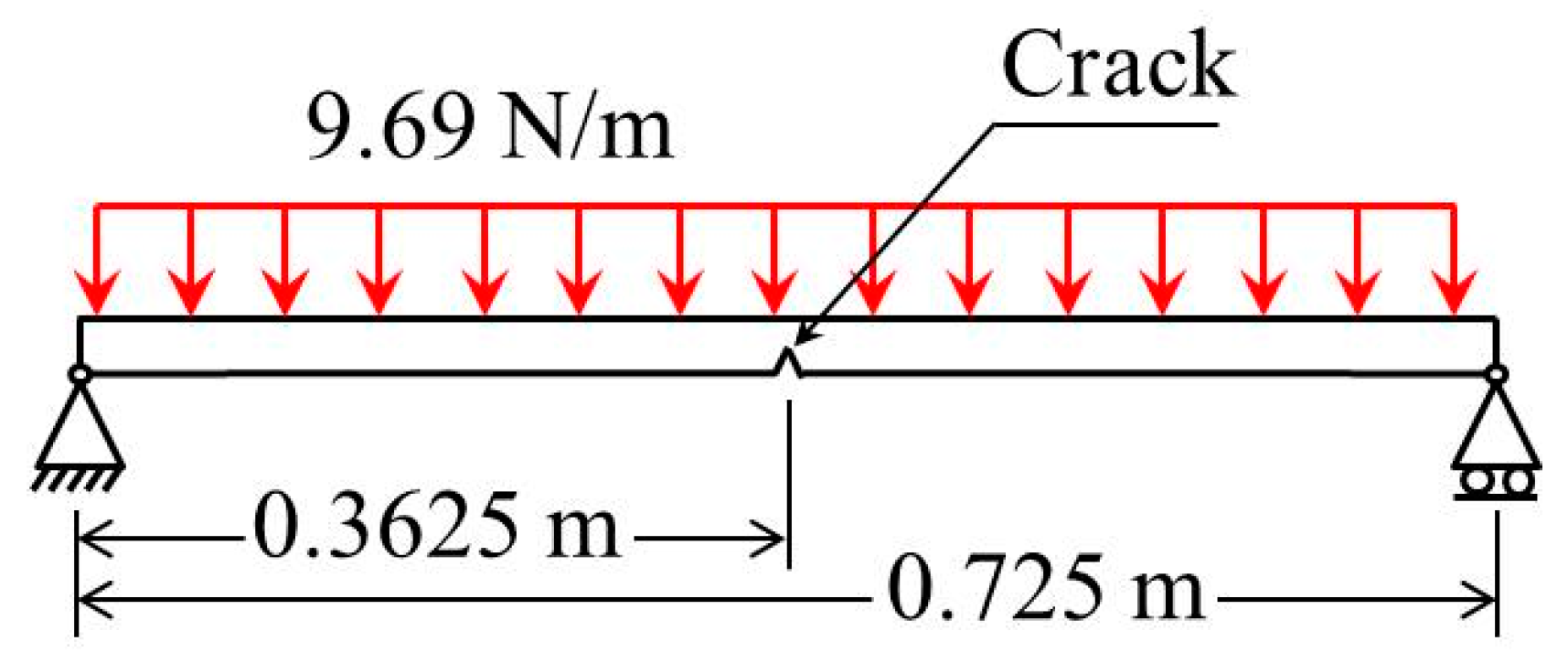
As a case study, a cracked rotor was investigated using a three-dimensional (3-D) finite element analysis in Abaqus/CAE. This study was conducted to show that non-symmetric bending principles should be used when analytically modelling the breathing response of a crack. The 3-D finite element model of the cracked rotor was devised in which the shaft is idealised as a beam with pin-roller supports and features a transverse crack at its mid-span as shown in Figure 1. The geometric and physical properties of the shaft are as follows: length L = 0.725 m, radius R = 6.35 mm. The shaft material was assumed to have a density ρ = 7800 kg/m3, Poisson’s ratio v = 0.3 and Modulus of Elasticity E = 200 GPa. Due to the shaft’s weight a uniformly distributed load of 9.69 N/m acts on the shaft along its entire length, where m is the mass of the shaft and g is the gravitational acceleration constant. The model does not consider dynamic loads so to simulate weight-dominant crack breathing [25]. As such, only the weight force is considered and is applied as a body force by specifying the material density and a gravity vector.
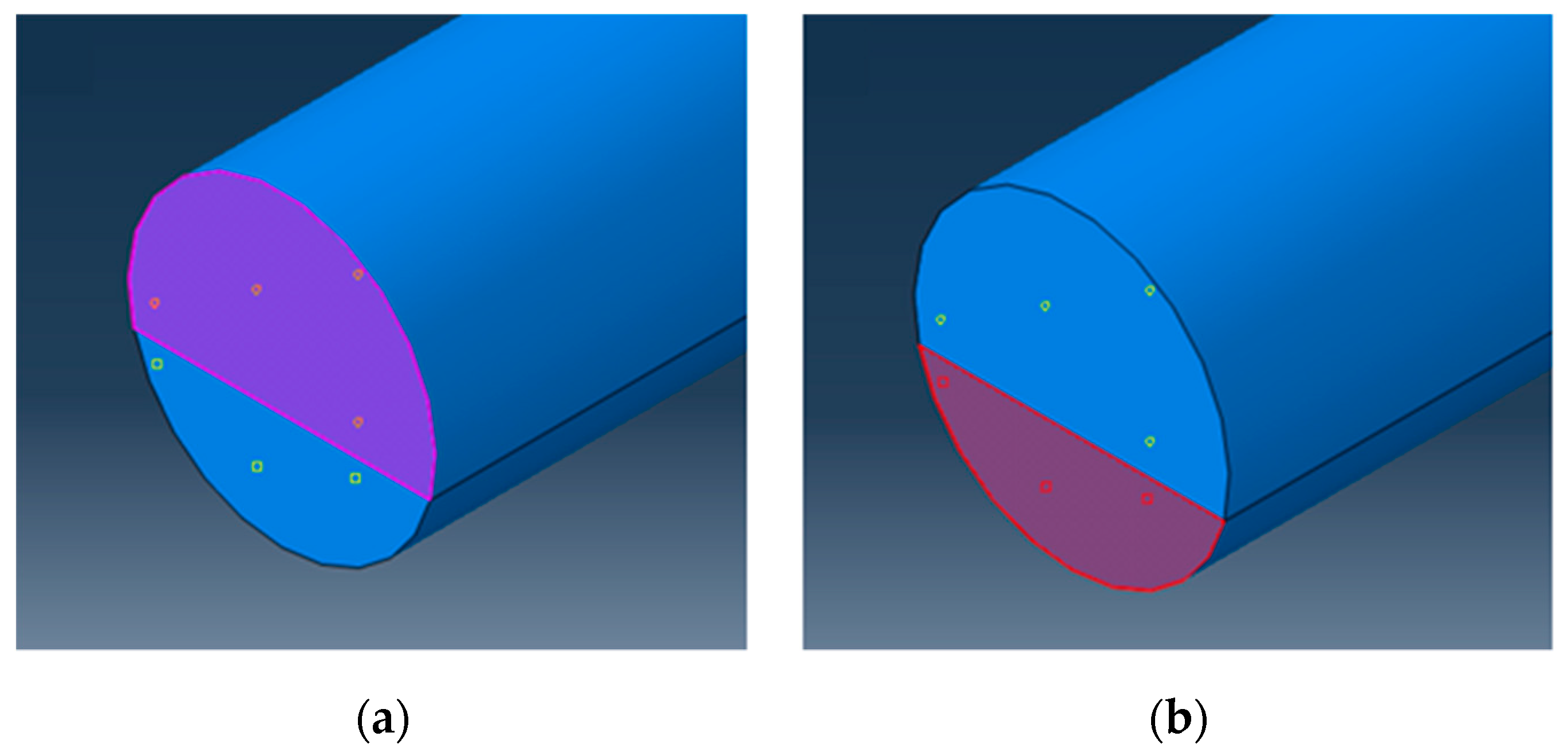
A transverse crack with a depth equal to 70% of the shaft radius was simulated by partially joining two solid shafts at one end by a tie constraint. This partially joined region, highlighted in Figure 2a, is representative of the undamaged (intact) section of the shaft. The purpose of the tie constraint is to lock the nodal displacements of the adjoining surfaces so no relative motion occurs between the two surfaces. The remaining unbonded regions represent the crack surfaces. A non-linear contact surface, highlighted in Figure 2b, is placed on one crack surface so that normal stress may be transmitted between the crack surfaces.
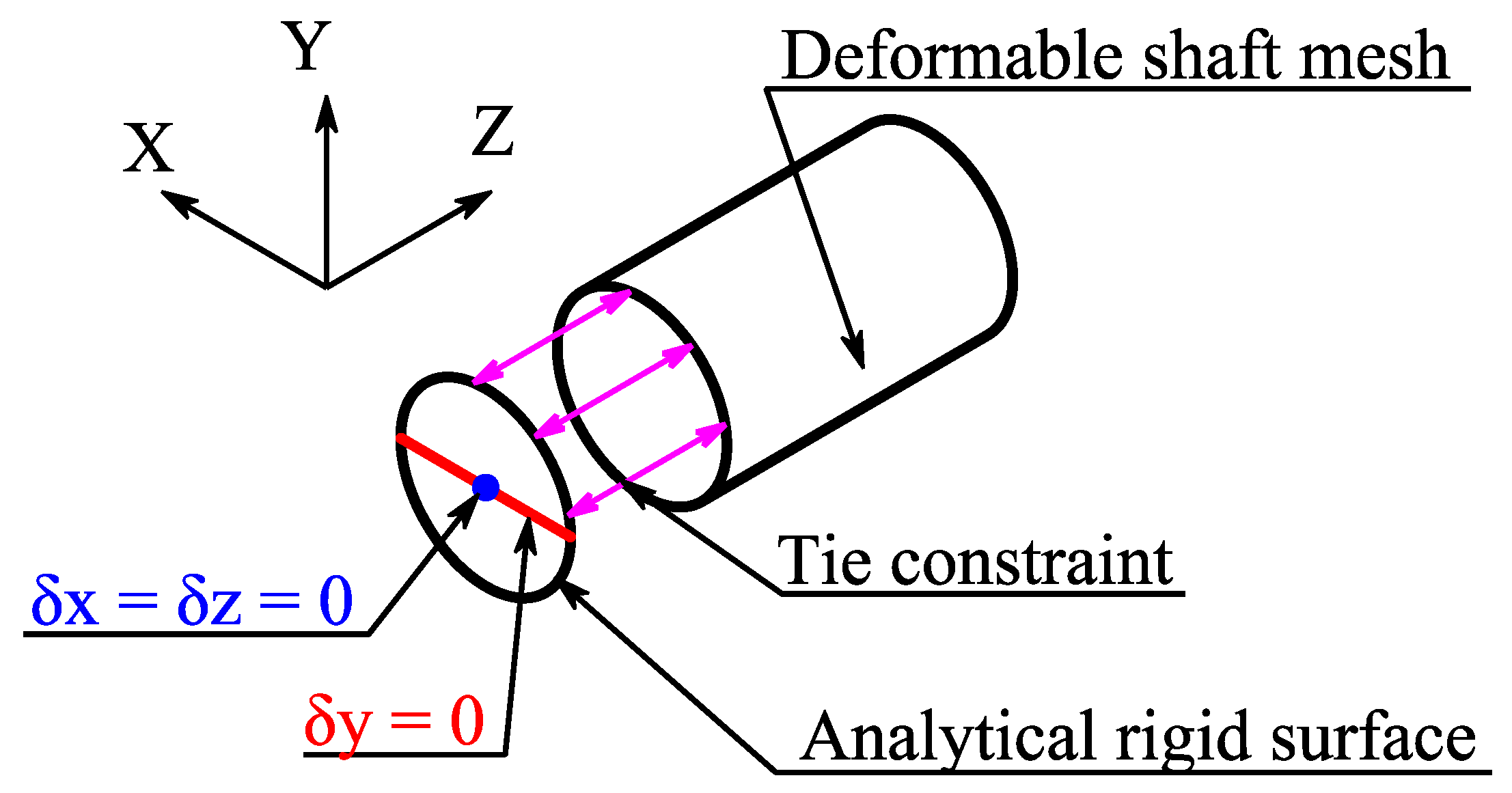
Due to the excessive local deformation and stress concentrations caused by directly applying pin-roller support boundary conditions at particular nodes, a rigid analytic surface was created as a separate part and bonded to the ends of the shaft using tie constraints, as shown in Figure 3. Furthermore, the degrees of freedom of the rigid analytical surface were constrained to a line and a point on the surface as shown, where the line constraint locked the mid-plane of the shaft end into the X–Z plane and prevented rotation about the Z axis and translation about the Y axis. The end of the shaft was still free to rotate about X and Y directions and free to translate in the X and Z directions. The point constraint locks the remaining translations leaving the shaft still free to rotate about the X and Y axes. Translation in the Z direction was only constrained at one end of the shaft to simulate an idealised pin and roller setup.
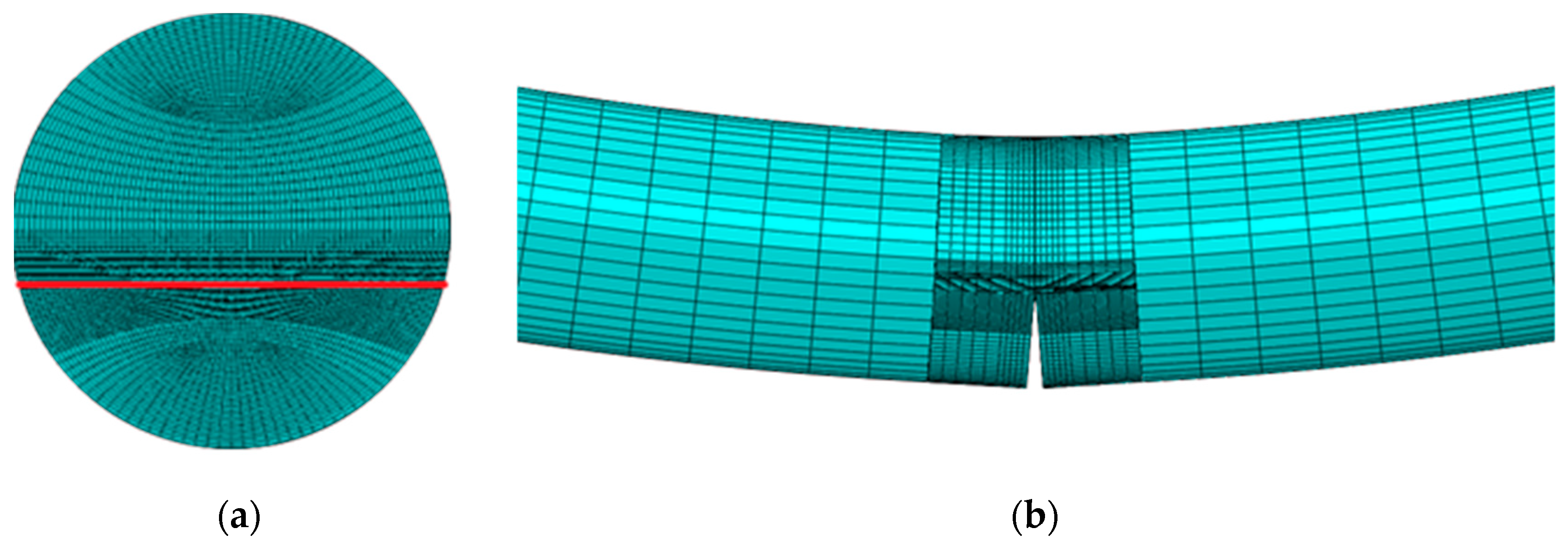
To reduce simulation time, the cracked region was modelled separately to the bulk of the shaft and then bonded to the bulk using tie constraints. Furthermore, the model’s element mesh was refined both radially and axially in the vicinity of the crack, where the degree of refinement was determined using a convergence test. The goal of the convergence test was to minimise simulation time without sacrificing too much simulation accuracy. The accuracy of the simulation was determined by analytically calculating the crack closing area and shaft deflection and comparing these to the FEA probed results. A summary of the convergence test is seen in Table 1. Mesh 9 (177,000 elements) was selected as it offered a high degree of refinement local to the crack whilst reducing the number of elements for the shaft bulk. The final mesh for the shaft bulk and immediate crack region can be seen in Figure 4.
The model was simulated by varying the shaft rotation angle from 0° to 345° in an increment of 15°. As the shaft rotates, the position of the crack changes relative to the neutral plane of bending. Any portion of the crack above and below the neutral axis experiences compressive and tensile stresses, respectively. Compressive stresses mean crack surfaces are under contact for crack closure while tensile stresses mean the crack surfaces are under separation for crack opening.
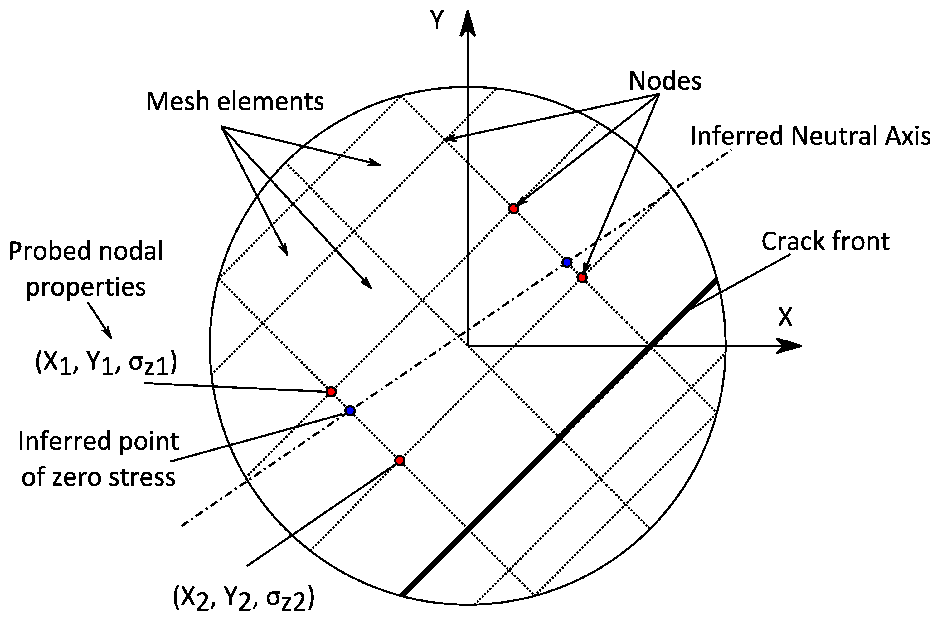
The neutral axis orientation angle at the crack location was identified by determining the coordinates of several nodes which have zero normal stress. Since the evaluated stress was rarely exactly zero at nodes, pairs of nodes with opposite stress signs that also shared an element edge were probed for their axial stress magnitude and spatial coordinates. According to the intermediate value theorem, there must be a point of zero stress, i.e., the neutral plane, and by using a linear trend line the location can be inferred. This idea is visualised in Figure 5.
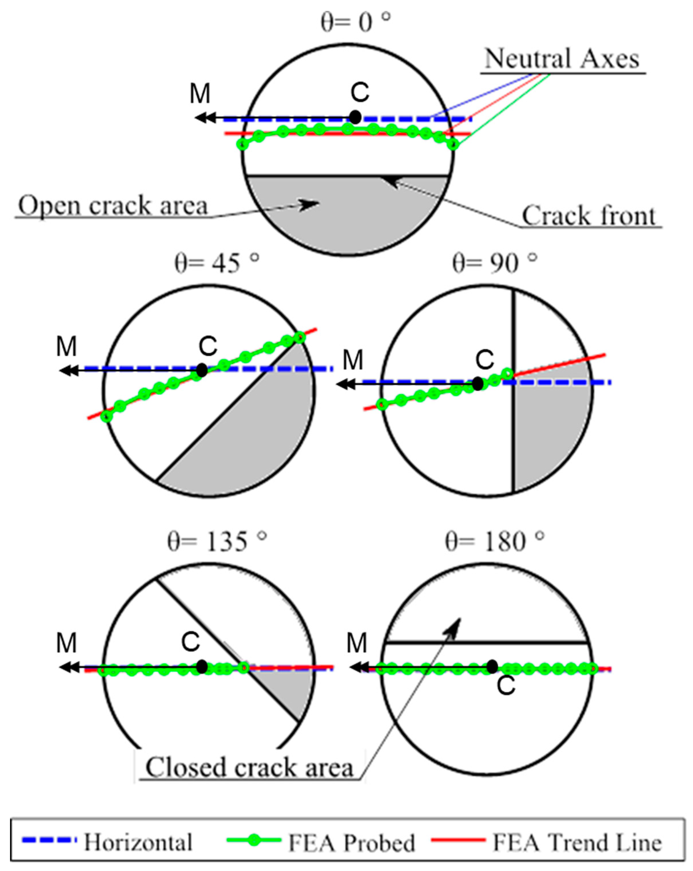
Figure 6 shows the neutral axis location and inclination for various shaft rotation angles (0°–180°). In this figure, the shaded region represents the open portion of the crack and the remaining region is the non-cracked area. It is assumed that the non-cracked area is the effective cross-sectional area at the location of the crack and the bending moment vector M acts horizontally about the centroid of the non-cracked area. The inclination angle of the neutral plane (from the horizontal) is non-zero when the shaft rotates to 45° (when the crack is fully open but the crack front is not horizontal) and to 90° and 135° (crack is partially open). According to beam theory [26], if the direction of the bending moment is not in a line with the planes of symmetry of a cross-section, then the neutral plane should be inclined relative to the symmetry planes. It is clear that the FEA probed values and trend line enforce this idea whenever the crack is partially open and therefore disagrees with the use of a horizontal neutral axis [12]. At the 0° and 180° cases, the non-cracked area is symmetrical relative to the direction of the bending moment and thus the FEA extracts that the trend line is horizontal. It should be noted that the numerically predicted trend line is included to reduce the semi-elliptical crack front to a straight crack front.
3. Development of Analytical Crack Breathing Model
The objective of this section is to develop an analytical model for determining the neutral axis position and to describe crack behaviour using non-symmetric bending principles. Understanding crack behaviour is useful for numerically determining the transient stiffness changes of the shaft local to the crack position and subsequently predicting the vibration behaviour of the shaft.
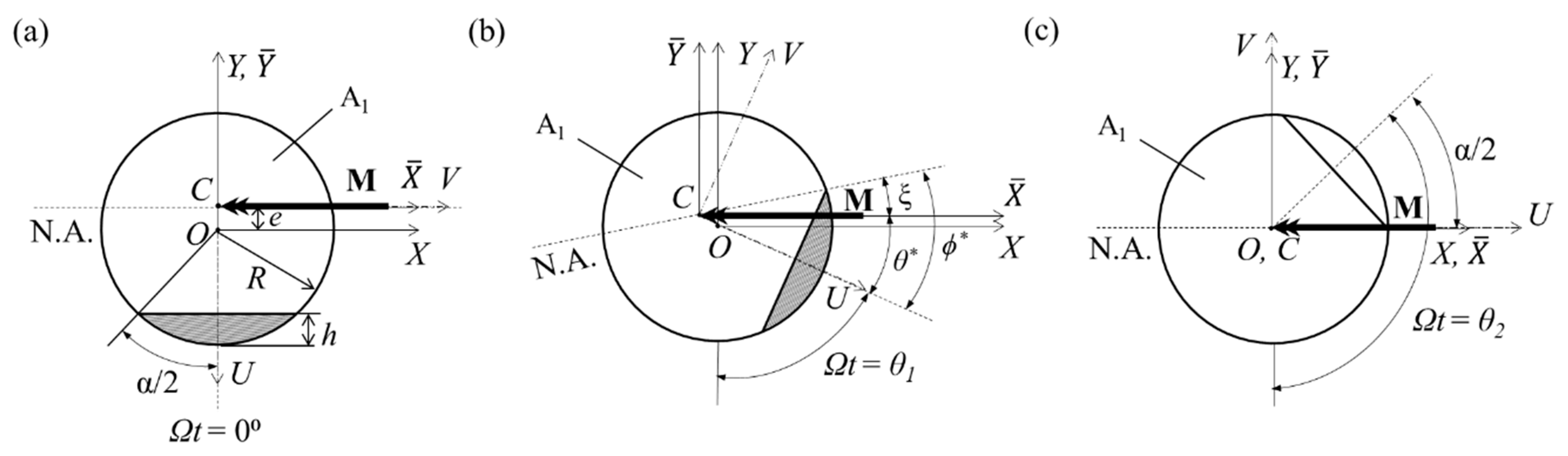
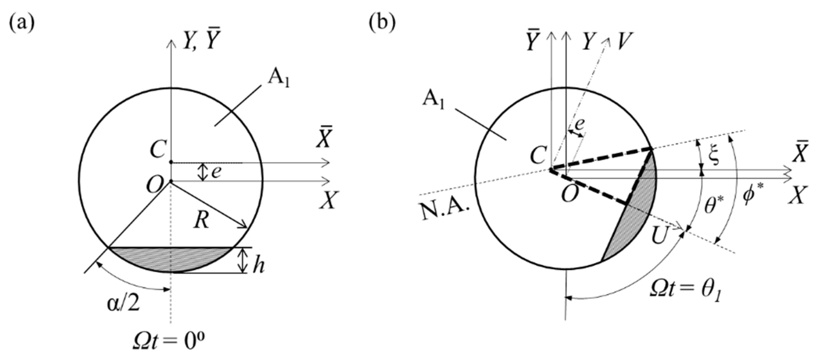
Consider a transverse cut through a shaft of radius R at the location of a straight-front fatigue crack. This transverse slice can be fashioned as shown in Figure 7a, where the shaded region depicts a fully open crack of depth h and the remaining region A1 is the undamaged area. The normalised crack depth μ is calculated by μ = h/R and the location of the crack in Figure 7a marks the initial position of the shaft (Ωt = 0°). Two Cartesian coordinate systems are established, the X–Y coordinate system remains fixed about the shaft centre O and the coordinate system whose centre remains coincident with the centroid of the non-cracked section C. Throughout the rotation of the shaft, the and axes remain parallel to the X and Y axes, respectively, and are therefore non-rotating. Moreover, the principal centroidal axes U and V are the first and second principal centroidal axes, respectively. The bending moment vector M acts upon C and its direction and magnitude are time-invariant as the model is assumed to be weight-dominant. In a weight-dominant model, only the weight of the rotor contributes to the breathing mechanism of the fatigue crack and any dynamic loads have a negligible contribution. The regions of the shaft above and below M are considered to be in compression and tension, respectively.
Furthermore, Figure 7 shows key milestones throughout the first half of the cracked shaft’s rotation, which is useful for determining the transient change in area moment of inertia of the cracked cross-section. Figure 7a shows a fully open crack (shaded crack) in the initial position with the crack front parallel to the neutral axis. The value of the intact area A1 is calculated by Equation (1) [11],
and the crack angle α/2 is derived to be
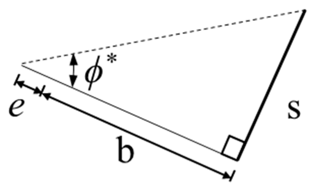
Moreover, the distance between the X and axes, denoted e, is given in [23] as
where is a convenience parameter. The position of the crack in Figure 7b depicts the instant that the crack begins closing; this angle is denoted as θ1. As such, for angles 0° ≤ Ωt ≤ θ1, the crack is considered to be fully open. During this range of angles (excluding Ωt = 0°), neither of the principal centroidal axes (U or V axes) is coincident with the bending moment vector, therefore, the neutral axis must be inclined relative to the bending direction, as shown. The angle between the first principal axis U and the bending moment vector, denoted θ*, is given as
Consequently, the angle between the first principal axis U and the neutral axis is given by Equation (5):
where IU and IV are the area moments of inertia of A1 about the principal centroidal axes [24]. When the crack is fully open, the values of IV and IU are equal to Ī1 and Ī2, respectively [12].
The angle of inclination of the neutral axis to the bending moment vector ξ is determined by
Now, the crack closing angle θ1 for this study can be numerically determined using Equation (9). Full derivation of this equation can be found in Appendix A.
For the horizontal neutral axis (HNA) model [12], the crack closing angle was determined as
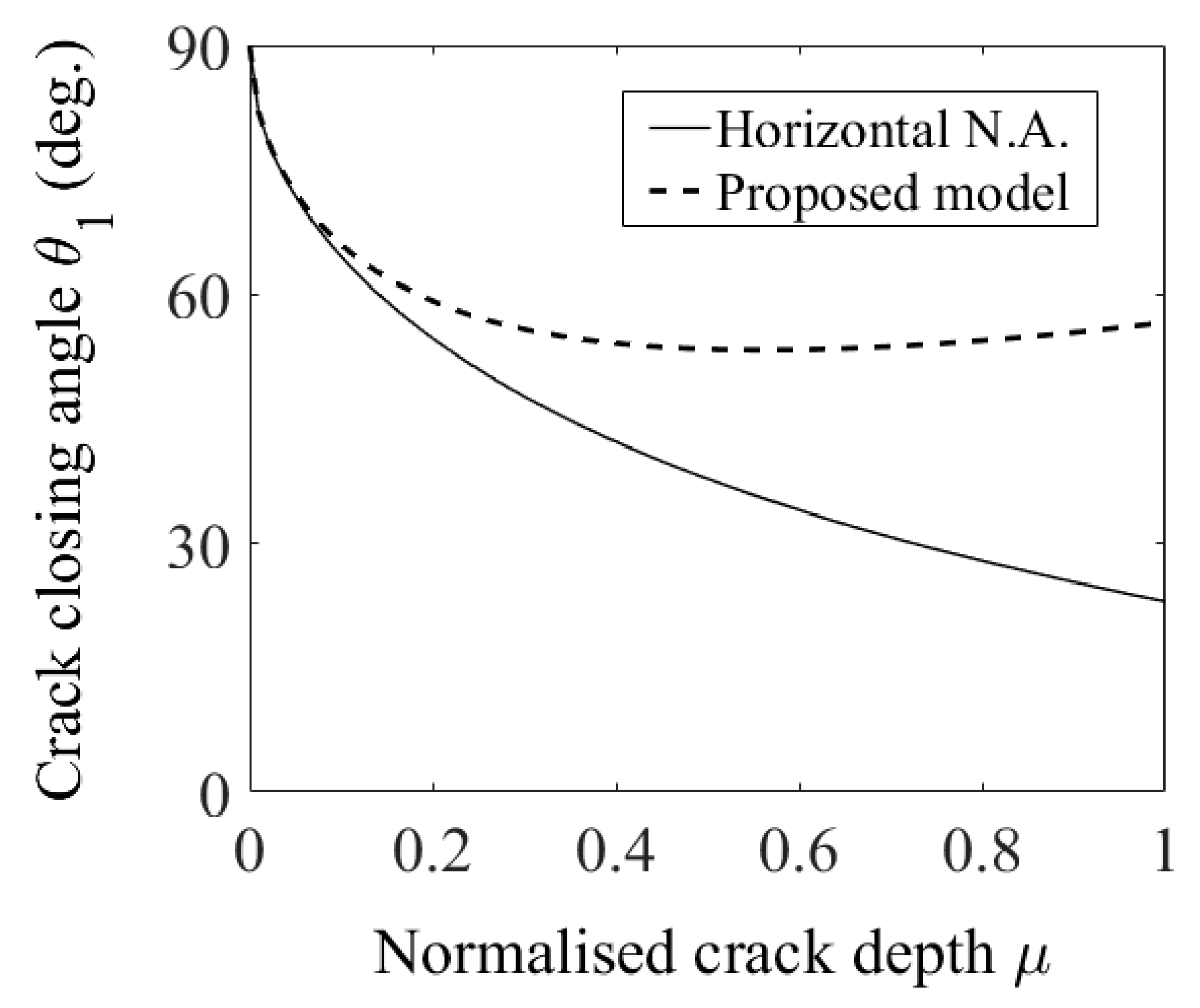
The comparison between Equations (9) and (10) for crack depths μ = 0 to μ = 1 is shown in Figure 8. There is a clear divergence between the two models with the proposed model showing that the crack closes later when compared to the HNA model. The difference in the predicted crack closing angle becomes more severe at deeper cracks, where at μ = 1, a 33.6° difference occurs (56.6° versus 23.0°). The comparison suggests that deeper cracks result in a more pronounced difference between the two models; hence, further investigations into the proposed model are valuable for deeper cracks.
Figure 7c depicts the instant the crack is completely in compression and thus becomes fully closed. This occurs when the shaft rotation angle is equal to θ2, where θ2 can be calculated by
It is worth noting that in the second half of the crack’s rotation, the crack remains closed until Ωt = 2π − θ2 and then gradually opens until Ωt = 2π − θ1, where it becomes fully opened again. Furthermore, the crack is partially open between these two angles. Table 2 summarises the crack status over one period of the shaft rotation.
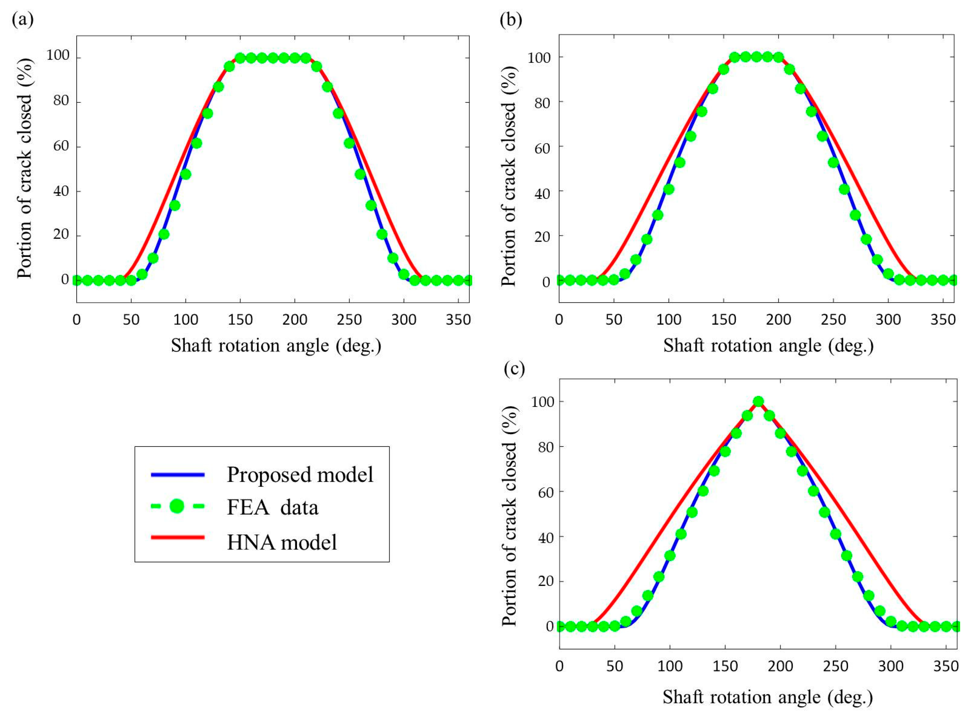
One method for illustrating crack breathing behaviour is to determine how much of the crack has closed as the shaft rotates, such as in Figure 9. To gauge the crack closing amount λ, the following formula was used
where à = πR2 (area of a full circle) and Ace is the total non-cracked area. For the presented model, the value of Ace was determined using the contents in Appendix A. Additionally, for the FEA model, the contact area of the crack was probed directly from the non-linear contact surface. At the crack depths chosen, μ = 0.5, μ = 0.7 and μ = 1.0, the proposed model begins closing later, i.e., λ increases from 0% at a higher shaft rotation angle. Moreover, the proposed model becomes fully open sooner, i.e., λ reaches 0% again sooner when compared to the HNA model; this is merely a consequence of the θ1 values being larger for the proposed model. Furthermore, the two crack models become fully closed at the same time, i.e., both models reach a λ value of 100%, and also begin opening again at the same time as the θ2 values are identical. As such, when the crack is partially open (λ is not 0% or 100%) the HNA model overestimates the closed area of the crack which results in stiffer cracked rotor models when predicting vibration. Furthermore, the deeper the crack the more pronounced the overestimation of θ1 becomes.
Additionally, knowing the state of a crack is essential for determining the area moments of inertia of the cracked cross-section, which, in turn, is used to quantify stiffness changes in the shaft. When the crack is fully closed the area moment of inertia of the total non-cracked cross-section will be at a maximum (equal to πR4) in the and directions ( and , respectively) and the product moment of area () is zero as the effective cross-section is a solid circle. (It should be noted that the product moment of area is linked to the local cross-coupling stiffness associated with the breathing crack.) When the crack is open to any degree, the area moment of inertia is non-maximum and product moment of area is non-zero and requires a more rigorous process to calculate.
The variation in and over one period of the shaft rotation can be accurately approximated by [12]:
where, and , known as breathing functions, are shape functions that reflect the changes in area moment of inertia over time. The breathing functions were derived in the following form using Fourier series approximation:
where p is a positive even integer related to the number of harmonics in the Fourier series. Equation (18) provides the breathing function for the product moment of area [27], where the parameter is given as . Since these Fourier series approximations were based on data that assume that the neutral axis remains horizontal, the procedure must be reinvestigated to apply non-symmetric bending principles.
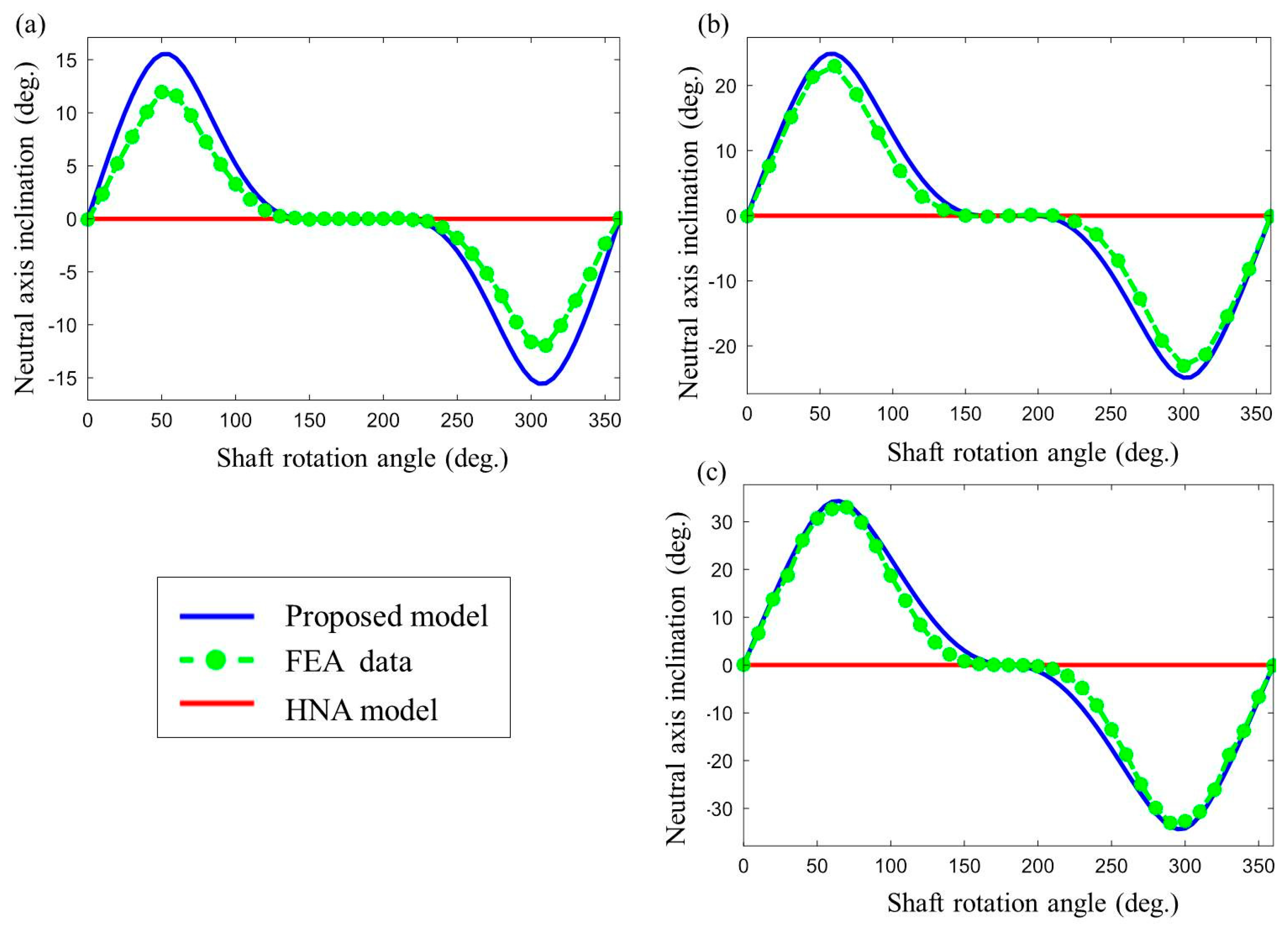
Appendix A amends the iterative geometric procedure [12] to determine the inclination angle of the neutral axis, based on the area moments of inertia and , repeatedly, until both are below a relative error threshold. Figure 10 shows the final neutral axis inclination angle at particular shaft rotation angles and for various crack depths. This result is juxtaposed with an unchanging horizontal neutral axis and superimposed with the FEA results, which was obtained by using the idea given in Figure 5. The foremost finding of the data is that the neutral axis is only horizontal when the crack is at the starting position or when fully closed and otherwise will shift from the horizontal. For the first half of the rotation, the inclination increases until θ1 and then decreases until becoming horizontal at θ2, in the second half the neutral axis remains horizontal until 2π−θ2 then becomes increasingly negative until 2π−θ1 and increases until the end of the period; a negative neutral axis value occurs when the neutral axis slopes below the positive axis. There is strong agreement between the proposed analytical derivation and the results obtained via FEA, with both sets of data showing that the peak inclination increases when cracks become deeper.
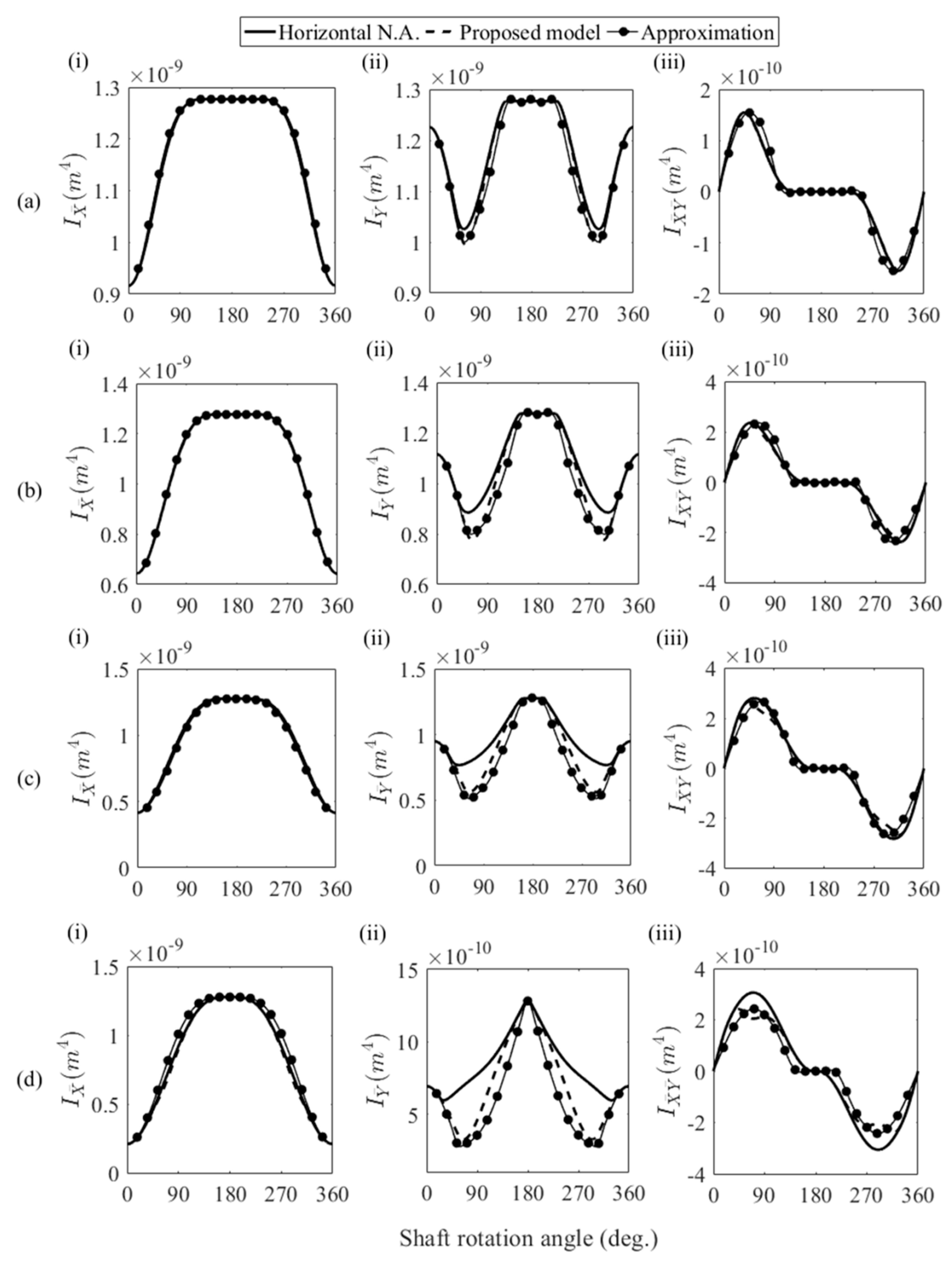
The development in Appendix A leads to the understanding that Equations (13)–(18) can be incorporated with non-symmetric bending principles as long as the proposed crack closing angle θ1 described in Equation (9) is used in lieu of Equation (10). This idea is evidenced in Figure 11 where the area moment of inertia of the total non-cracked cross-section obtained through Appendix A is compared to the iterative procedure [12]. The figure shows the result of substituting the proposed θ1 value into the Fourier series approximations of Equations (13)–(18) with p = 6 for and p = 10 for and . While not shown, the approximate model was found to be sufficiently accurate for all p values from 4 to 16. Additionally, when comparing the results in Appendix A to those from the iterative procedure [12], it is revealed that there is a negligible difference between values, a miniscule difference between the product moment of area and a pronounced difference occurs between the prediction of for all the crack depths examined (μ = 0.3, 0.5 and 0.7, 1.0). In particular, the proposed model produces smaller values than the HNA model when both models are neither fully open nor fully closed and this difference becomes more significant the deeper the crack.
Since the proposed model and the HNA model show a divergence in area moment of inertia at deeper cracks, the predicted stiffness changes in the cracked shaft may be sufficiently different between the two models. Therefore, an investigation into the vibration behaviour of a cracked rotor with mid-to-late-stage cracks should be further investigated.
4. Two-Dimensional Finite Element Modelling and Vibration Analysis of Cracked Rotor
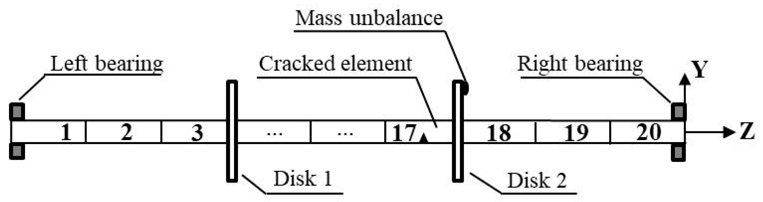
The schematic in Figure 12 is representative of a cracked rotor model with two disks, supported by isotropic rolling-element bearings at both ends (nodes 1 and 21). The two-dimensional (2-D) finite element model is discretised into twenty Euler-Bernoulli beam elements (N = 20), where Element 17 is the cracked element and nodes 4 and 18 carry Disk 1 and Disk 2, respectively. An unbalanced mass with an unbalance eccentricity of 1 × 10⁻⁵ kg∙m at an angle of 0° is attached to Disk 2. The physical specifications and bearing properties of the rotor are shown in Table 3 and Table 4, respectively.
The stiffness matrix of a homogenous Euler-Bernoulli beam element is written as
where E is the elastic modulus of the shaft and l is the length of the cracked element [26]. The stiffness changes due to the breathing crack can be directly described by evaluating Equation (19) at chosen time intervals. Alternatively, applying a coordinate transformation to the and axes allows the already derived , and values to be used instead of the principle area moments of inertia. This is achieved by
where is the resulting cracked stiffness matrix about the and axes and is the transformation matrix given by Equation (21),
The parameter αp is the rotation angle between the coordinate system and the principal centroidal coordinate system. The result of Equation (20) is equivalent to
which can be achieved by applying double angle formulas and the following equations,
derived from Mohr’s circle for area moments of inertia [28]. Importantly, IUV = 0 since the U-V plane is the principal plane.
Substituting Equations (13)–(15) into Equation (22) then partitioning the resulting matrix based on the breathing functions will yield
It should be noted that is related to the stiffness of the intact area of the cracked cross section, and are stiffness contributions of the breathing crack in the and directions, respectively, and is related to the cross-coupling stiffness contribution of the breathing crack. The matrices , , and are given by
where , and . It should be noted the final expression of is independent of αp so the angle does not need to be determined.
The stiffness element matrix for the non-cracked elements, as well as the mass and damping/gyroscopic matrices for all the shaft elements, disk and rolling-element bearings can be found in literature [29].
The equation of motion associated with the cracked rotor system is described by
where M, C, G, K0, K1, K2 and K3 are global matrices of size 4 (N + 1) × 4 (N + 1) relating to the mass, damping, gyroscopic effect, , , and , respectively. The global matrices are assembled using a standard finite element modelling procedure [29]. The assembly of K0 includes the stiffness of all the shaft elements; however, stiffness element entries associated with the cracked element are replaced by those in . Additionally, K1, K2 and K3, are sparse matrices whose only non-zero elements correspond to the values of , and , respectively. The 4 (N + 1) × 1 displacement vector q(t) describes the nodal translations and nodal rotations about the X and Y axes. The 4 (N + 1) × 1 vector F1 and F2 are the unbalance amplitude vectors and Fg is the weight force vector [11].
The equations of motion of the cracked rotor system can be solved by using a harmonic balance procedure by assuming that the solution of q(t) is in the following form:
where n is the number of harmonics for the solution q(t) and the breathing functions f1(t), f2(t) and f3(t) are written in the following forms:
where p is the number of harmonics for the breathing functions. The harmonic balance procedure involves the substitution of Equation (31) and its time-derivatives as well as Equations (32)–(34) into Equation (30). After equating the coefficients of harmonics, the following form can be achieved:
where n is the number of harmonics chosen, , for i = 1, 2, 3,…, n, for i = 1, 2, 3, …, n, for i = 1, 3, 5, …, 2n−1, for i = 2, 4, 6, …, 2n, for i = 1, 3, 5, …, 2n − 1, for i = 2, 4, 6, …, 2n, for k = 1, 3, 5, …, 2n−3 and i = 1, 2, 3, …, n − 1, for k = 2, 4, 6, …, 2n − 2 and i = 1, 2, 3, …, n − 1, for k = 1, 3, 5, …, 2n−3 and i = 1, 2, 3, …, n − 1, for k = 2, 4, 6, …, 2n−2 and i = 1, 2, 3, …, n − 1. The symbol corresponds to a 4 (N + 1) × 1 vector of zeroes. The square coefficient matrix (i.e., the N (2n + 1) × N (2n + 1) matrix) of Equation (35) is referred to as δ herein. The solution to Equation (35) involves determining the vector , where each term is a 4 (N + 1) × 1 vector of amplitudes containing all nodal translations and rotations. Vector A0 corresponds to the amplitude of non-harmonic terms, vectors A1 through An correspond to the amplitudes of cosine multiples, i.e., Ancos(nΩt) and vectors B1 through Bn correspond to the amplitudes of sine multiples, i.e., Bnsin(nΩt). The frequency amplitude of each nodal degree of freedom is defined as the vector sum of the corresponding cosine and sine amplitudes of the same frequency, i.e., .
The critical speeds of the cracked rotor in Figure 12 were determined by first identifying the damped natural frequencies at a series of rotor spin speed values (0–40,000 rpm). This process involves calculating the eigenvalues of seen in Equation (36):
where is the first-order system corresponding to Equation (30), is an 4 (N + 1) × 4(N + 1) matrix of zeroes and I is the 4 (N + 1) × 4 (N + 1) identity matrix. Since the stiffness K0 is used, the eigenvalue solutions of provides the damped natural frequency of a rotor with a non-breathing open crack.
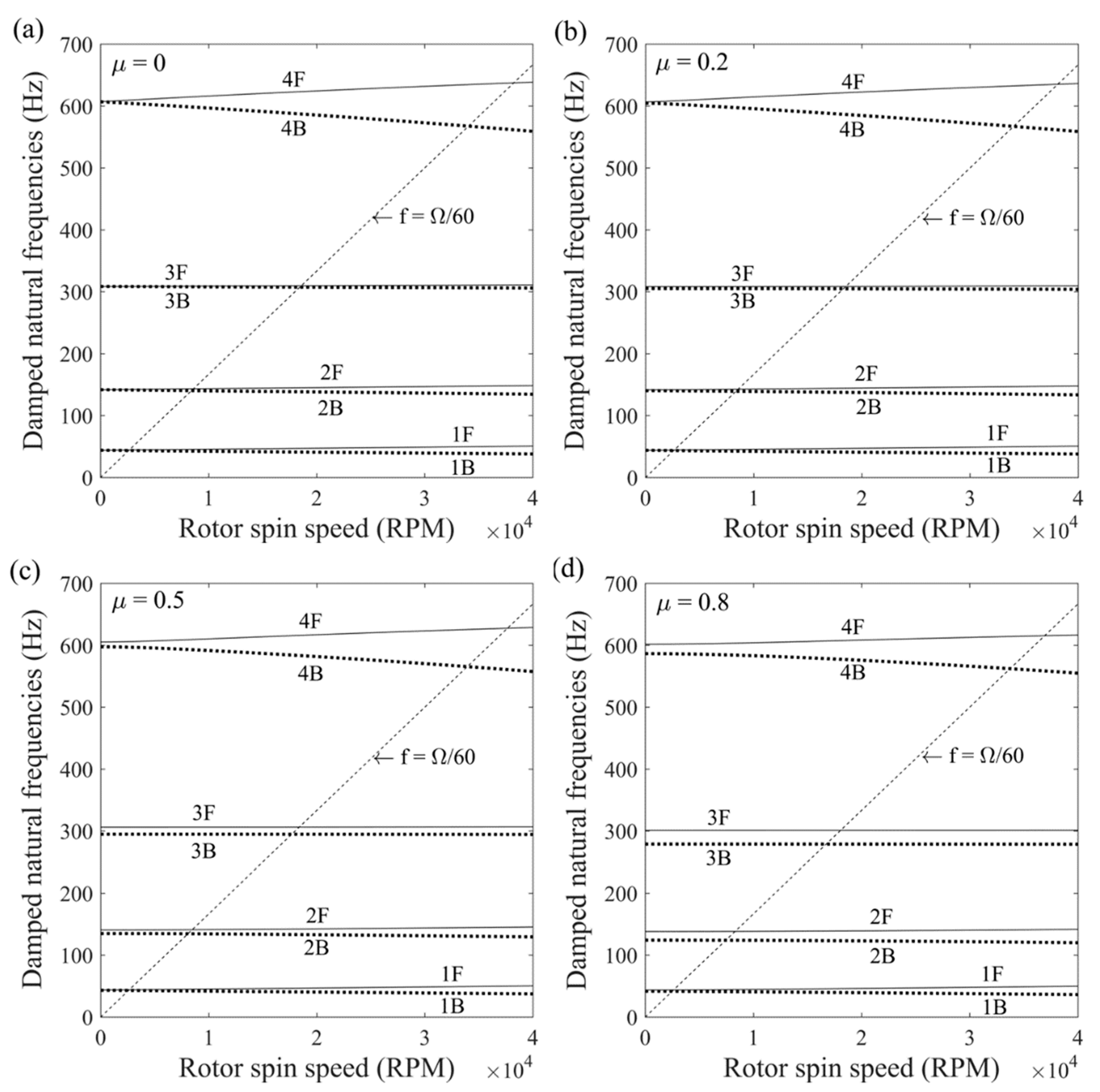
The Campbell diagrams in Figure 13 illustrate the change in the first four forwards and backwards damped natural frequencies (given in Hz) with an increase in rotor spin speed (given in rev/min) for open cracks of different depths, namely μ = 0, 0.2, 0.5 and 0.8. These crack depths were chosen as μ = 0 means no crack is present, μ = 0.2 is an early/mid stage crack, μ = 0.5 is a mid-stage crack and μ = 0.8 is a late stage crack. The notation ‘nB’ and ‘nF’ refers to the backwards and forwards damped natural frequencies for order n, respectively; for example, 2B is the second backwards damped natural frequency and 3F is third forwards damped natural frequency. It is explained in literature [29,30] that backwards whirl modes result in a lower damped natural frequency relative to forward whirl modes due to the gyroscopic effect of the rotor disks and therefore the two curves will diverge from one another. Additionally, Figure 13b–d shows that for cracked rotors each corresponding forwards and backwards whirl frequency lines are separated at zero RPM, whereas for an undamaged shaft (Figure 13a), the frequency value at zero RPM is identical. Furthermore, the asymmetry of the open crack cross section and corresponding stiffness asymmetries causes the backwards and forwards natural frequency pairs to further separate. Figure 13 also features a diagonally spanning dotted line representative of the first-order excitation. The intersection points between the excitation line and the damped natural frequency lines determine the set of forward and backward critical speeds of each rotor. Table 5 summarises the critical speed values found according to Figure 13.
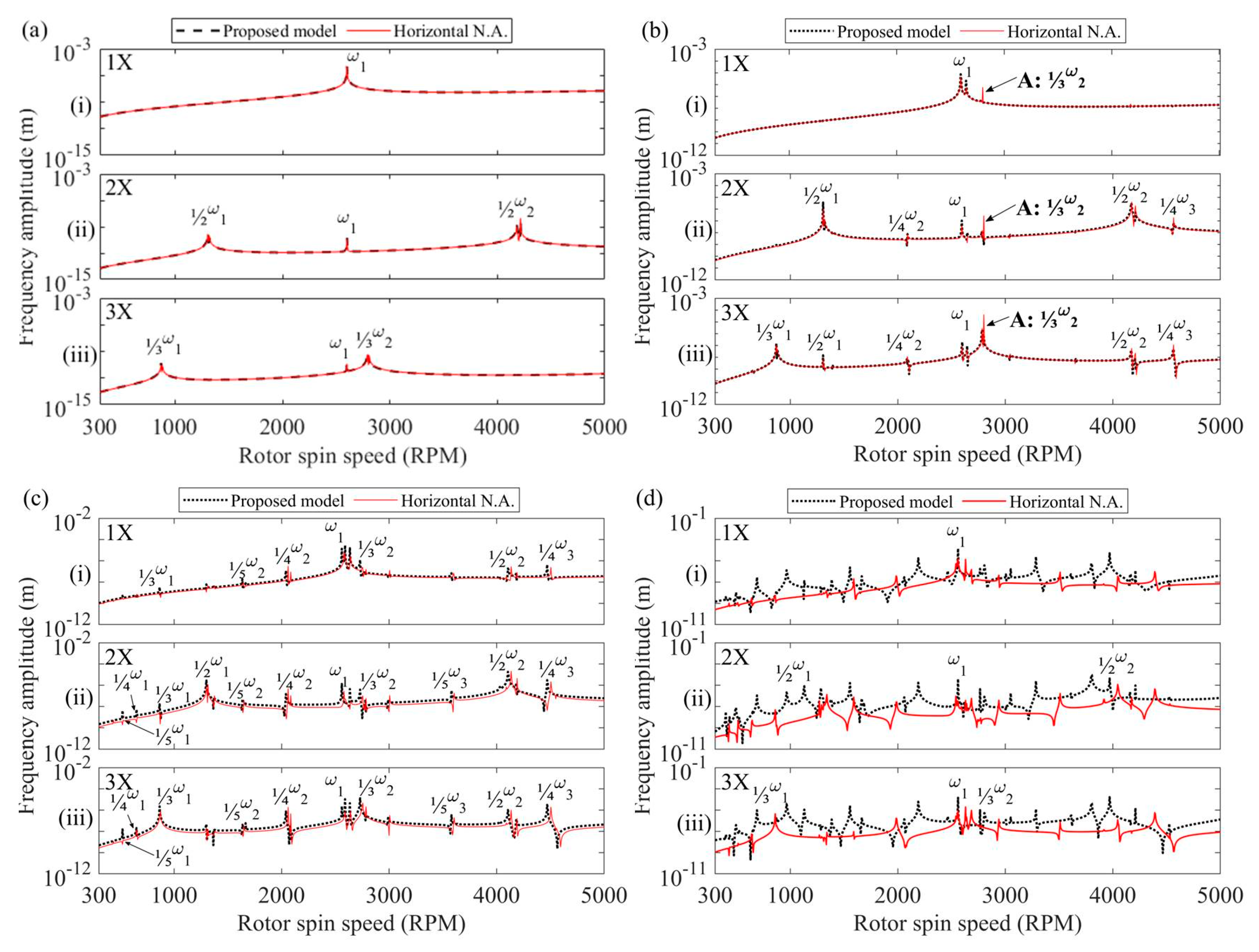
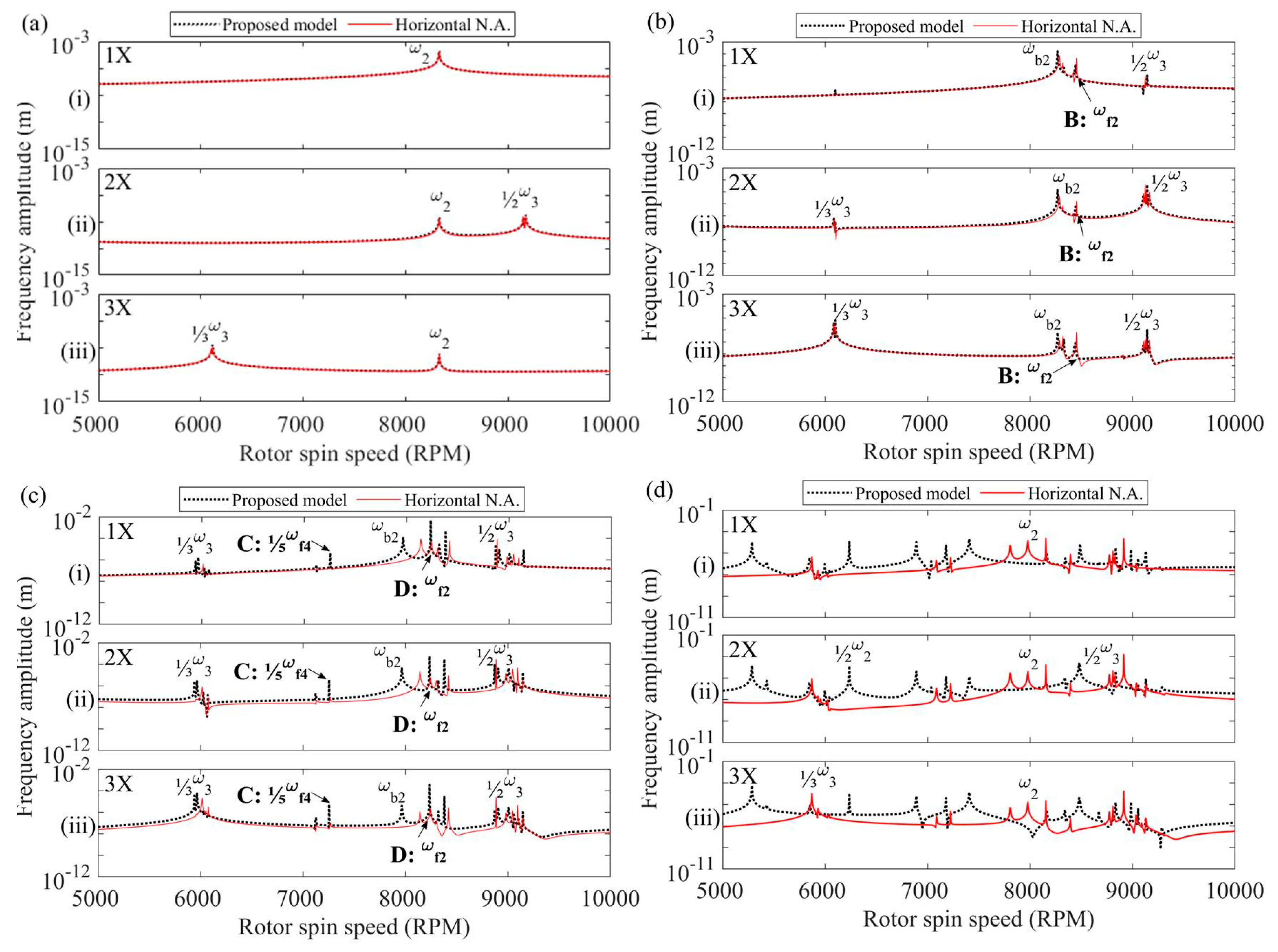
Figure 14 and Figure 15 show the vertical amplitude (Y-direction) of Node 1 for the first three harmonic frequency components predicted by the proposed model and the chosen HNA model. Rotor spin speeds within the vicinity of the first and second critical speeds were chosen, as well as crack depths of μ = 0, 0.2, 0.5 and 0.8. The series of peaks in frequency amplitude that appear throughout the figures approximately correspond to discrete fractions of the critical whirl speeds shown in Table 5, for example, ⅓ωf2 is one-third of the second forwards critical speed. These peaks occur in pairs where the left and right peaks correspond to a discrete fraction of a particular backwards and forwards critical speed, respectively. At times, these peaks appear to be singular due to the closeness of the peaks and inadequate granularity of the horizontal-axis and so are labelled without ‘b’ and ‘f’, for example ‘⅓ω2′ instead of ‘⅓ωf2′ and ‘⅓ωb2′. Moreover, the isolated peaks may be due to the pair of peaks being greatly different in value.
For an undamaged shaft (μ = 0), both models show that a peak occurs at the first and second critical speeds, ω1 and ω2, for the 1X, 2X and 3X frequencies. Furthermore, for the 2X and 3X frequencies, peaks occur at one-half and one-third the first three critical speeds, respectively. The occurrence of these peaks is therefore unrelated to fatigue cracks; however, it is known in the literature that the magnitude of these peaks may increase depending on unbalance [31] and crack depth [32,33].
For crack depths of μ = 0.2 and 0.5, peaks relating to other discrete fractions of critical speeds arise in addition to the aforementioned peaks. As the crack deepens, the magnitude of these additional peaks increases, suggesting that these peaks are related to the presence of fatigue cracks. In fact, Figure 14 and Figure 15 show that there is an overall increase in the magnitudes of the 2X and 3X components for μ = 0.2, 0.5 and 0.8 relative to no crack. An upwards trending increase to the 2X and 3X components is well known in the literature as a theoretical and practical method for determining the presence of fatigue cracks [2].
With regards to magnitude, the 1X, 2X and 3X frequency amplitudes predicted by the two models are identical or approximately equal for crack depths of μ = 0, 0.2 and 0.5. However, at particular rotor speeds, the two models significantly differ in magnitude, such as at points of interest A, B, C and D seen in Figure 14b and Figure 15b,c, respectively.
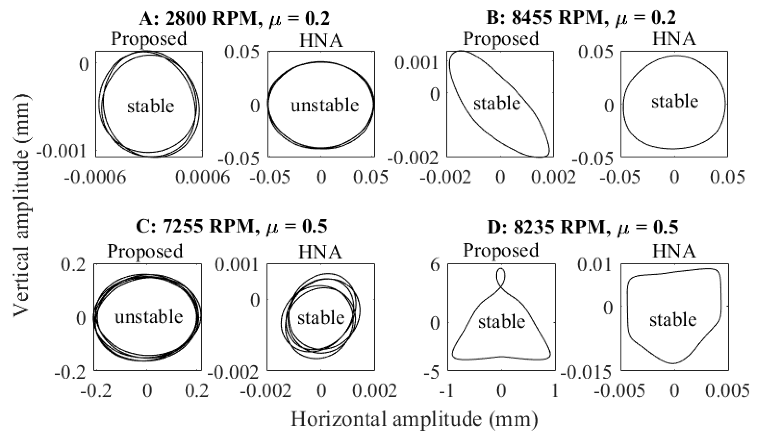
Since numerical instability can lead to misleading results, the numerical stability of the rotor dynamic solutions at the points of interest was examined. The numerical stability of a cracked rotor can be found quickly in the frequency domain by identifying the sign of the determinant after scaling the coefficient matrix δ in Equation (35), as shown in [34]. Figure 16 displays the transverse trajectory of Node 1 at the four points of interest and also indicates the numerical stability of the solution, or lack thereof. It was found that at point of interest A (2800 rpm, μ = 0.2), the HNA model’s solution was numerically unstable; however, the proposed model’s solution was stable. Conversely, the proposed model was unstable and the HNA model was stable at point C (7255 rpm, μ = 0.5). Visual inspection of points A and C in Figure 14 and Figure 15 show that these peaks rise sharply and suddenly occur (as opposed to gradually forming) and the other model does not predict a sudden peak at the corresponding rotor speed. Therefore, it is suggested that these peaks occur due to numerical instability and thus explains the difference between the two models at these points of interest. On a side note, the similarities between the two models for early/mid staged cracks (μ = 0.2 and 0.5) may be exploited to determine a numerically stable vibration solution when only one model is found to produce an unstable result. In contrast, both the proposed model and the HNA model had stable solutions for points of interest B (8455 rpm, μ = 0.2) and D (8235 rpm, μ = 0.5), suggesting that the small difference in the breathing mechanics of the two crack models is sufficient to result in relatively different vibration behaviour for early/mid stage cracks (μ = 0.2 and 0.5). Furthermore, the transverse trajectory of Node 1 at points of interest B and D also differed in shape; therefore, these points of interest may be a meaningful indicator when experimentally validating the proposed model.
Figure 14d and Figure 15d show the 1X, 2X and 3X frequency amplitudes for the two models at a crack of depth μ = 0.8. Across all three frequencies, both models have no clear global maximum amplitude value due to the appearance of a high number of amplitude peaks and also both models have very few rotor speeds for which a common peak occurs. It is assumed that this overall difference in the predicted vibration stems from the largely differing breathing behaviour found for the deep cracks. Therefore, the proposed model may be valuable for the simulation or detection of mid to late staged cracks (μ = 0.5 and deeper). Moreover, the significant asymmetry of the deeply cracked cross-section is a likely source of the increased number of discrete fractional peaks that appear. These additional peaks may be used as indicators for the presence of fatigue cracks for sufficiently deeply cracked rotors.
5. Conclusions
The 3-D FEA cracked rotor model herein demonstrated that the neutral axis of bending for a cracked cross-section cannot remain horizontal. This preliminary investigation showed that the neutral axis inclination angle increases from horizontal as the crack rotates depending on the openness of the crack. In response to this finding, the new breathing model was developed using non-symmetric beam bending theory to determine the changes in the geometry of the breathing crack. The analytical model supports the preliminary findings regarding a shifting neutral axis and also that the peak inclination angle value increased as the crack became deeper. In fact, the neutral axis is only seen to be horizontal when the crack is at its starting position or fully closed.
Due to the time-varying neutral axis a new formula for the crack closing angle θ1 was derived out of necessity. It was found that values θ1 calculated through the proposed formula diverged from an existing formula [12] as the crack deepened, where at a crack depth of μ = 1 there was a significant difference of 33.6°. As a result, for the proposed model, the crack begins closing later in its rotation and re-opening sooner and so the cracked shaft would be less stiff in bending when compared to the HNA model. This change in behaviour was most clearly manifested through the predicted values of the two models, where the proposed model had overall lower values for μ = 0.3, 0.5 and 0.7 and particularly more so for the deeper cracks.
As for the 2-D FE vibration analysis of the cracked rotor using the harmonic balance method, the vertical amplitudes of the first three harmonic components (1X, 2X and 3X) were focused on. The proposed crack breathing model was found to be highly similar to the HNA model for the case of no crack, μ = 0.2 and μ = 0.5 except at particular rotor speeds referred to as points of interest. Four points of interest were chosen and it was found that at two points of interest, the two models differed because of the numerical instability of either model and the other two points had largely different amplitudes without numerical instabilities. Having differences without numerical instability suggests that the difference in crack breathing behaviour between the two models has some value for predicting the vibration of cracked rotors with early-mid-stage cracks. Furthermore, the differing transverse trajectory predicted between the two models is suggested as a potential indicator for experimental validation of the proposed model. As a side note, both models predicted an appreciable increase in the amplitude of the 1X, 2X and 3X frequencies and an increase in amplitude peaks at discrete fractions of the first through third critical speeds as the crack deepened. Both of these factors are typical indicators for the presence of fatigue cracks in rotating shafts. The 1X, 2X and 3X amplitudes at μ = 0.8 resulted in a substantial difference between the two models where virtually no common amplitude peaks occurred. The proposed crack breathing model may be useful to capture the dynamic behaviour of rotors with mid-to-late-stage cracks once it is experimentally validated, which could be part of future work for continuation.
Author Contributions
J.S. created the finite element models and conducted simulations to extract the numerical results as the Ph.D. student and also drafted the paper. H.W. and C.Y. helped with data analysis, technical discussions and revision of the paper. All the authors contributed to results and discussions and commented on the paper. All authors have read and agreed to the published version of the manuscript.
Funding
The first author was supported by the Postgraduate Scholarship Awards provided by the Western Sydney University. This support is greatly appreciated.
Acknowledgments
The authors would like to show gratitude to Declan Williams and Mobarak Hossain for their valuable discussions on devising the cracked rotor model in Abaqus/CAE.
Conflicts of Interest
The authors declare no conflict of interest.
Appendix A
Figure A1a shows the crack in the starting position. From this position, the non-cracked area can be given by [12]:
also the radial distance of the centroid of area A1 from the origin O is
The area moment of inertia of the crack segment about the X and Y axes are
The area moment of inertia of non-cracked segment A1 about the X and Y axes, respectively, are
where, I = πR4/4. Using the parallel axis theorem, the area moment of inertia of A1 about the and axes yields
Appendix A.1. Fully Open Crack Equations
These equations are only valid for 0 ≤ Ωt ≤ θ1 and 2π−θ1 ≤ Ωt ≤ 2π.
Using Figure A1b, the distance between the Y and axes is denoted Xce and the distance between the X and axis is Yce and these values are calculated by
Additionally, for a fully open crack the total non-cracked area is equivalent to A1
the angle between the first principal axis U and the bending moment vector θ* and is given as
Furthermore, in [24], the angle between the first principal axis U and the neutral axis is given by
where IU and IV are the area moments of inertia of A1 about the principal centroidal axes. The angle of inclination of the neutral axis to the bending moment vector ξ is determined by
For a fully open crack the - plane is rotated by Ωt clockwise from the principal plane. As such, the product and area moment of inertia of the uncracked area about the and axes are
At the instant the crack begins closing (Ωt = θ1), the leading vertex of the crack becomes coincident with the neutral axis, creating a right-angled triangular region bounded by half of the crack front and the U-axis, as seen in Figure A1b; this region has been isolated in Figure A2, where
and and (these identities are provided in [12]).
Figure A1.
Fully open shaft crack at the (a) starting position and (b) instant the crack begins closing.
Figure A1.
Fully open shaft crack at the (a) starting position and (b) instant the crack begins closing.

Figure A2.
Triangle bounded by bold-dashed lines seen in Figure A1.
Figure A2.
Triangle bounded by bold-dashed lines seen in Figure A1.

Substituting Equation (A13) into Equation (A18), knowing that and , results in
Substituting Equation (A12) into Equation (A19) and θ1 for Ωt gives
Appendix A.2. Fully Closed Crack Calculations
These equations are only valid for θ2 ≤ Ωt ≤ 2π−θ2.
The effective geometry of the transverse slice for a fully closed crack is a solid circle. Which means that following is true: , , , and .
Appendix A.3. Partially Open Crack Calculations
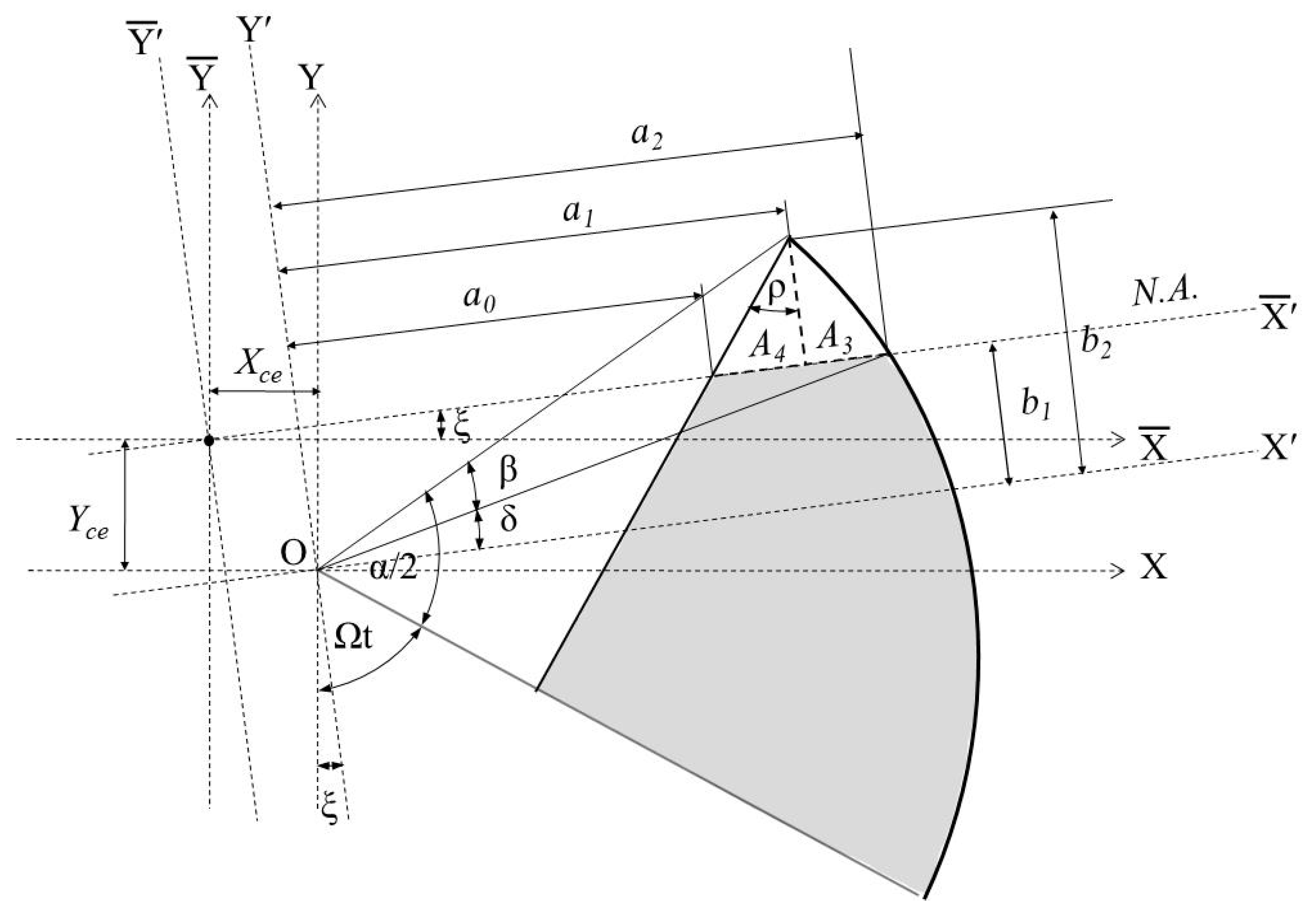
Figure A3 is representative of a crack at some angle Ωt = θ1 + ε, where ε is a very small angle ensuring that θ1 < Ωt + ε << θ2. A small portion of the crack segment passes over the neutral axis into the compressive field and therefore closing this portion of the crack. This portion can be split into areas A3 and A4.
Figure A3.
Geometry of a partially open crack and relevant coordinate axis systems.

The objective is to determine the product moment of area and area moment of inertia of the total non-cracked region about the and axes. A similar derivation process to the one in [12] will be used, however modifications are necessary due to the inclined neutral axis. Ergo, two rotated axis coordinate systems must be introduced, i.e., and and also X′ and Y′ which are rotated by ξ from and axes and X and Y axes, respectively. Figure A4 should be examined first to provide context to the following formulae:
The shape and area of A3 and A4 are dependent on the following angles
The boundary points of A3 and A4 about the X′ and Y′ axes are given as
By iteration, the following values should be refined at each Ωt increment before proceeding: properties pertaining to A3 in relation to the X′ and Y′ axes are
The properties pertaining to A4 in relation to the X′ and Y′ axes are
and the properties pertaining to A1 in relation to the X′ and Y′ axes are
Therefore the properties pertaining to the total non-cracked area Ace in relation to the X′ and Y′ axes are
After refined values for and are obtained, the product and area moment of inertia values about the X′ and Y′ axes for A3 are determined by
the following equations are for A4
and for A1
The product and area moment of inertia values for the total non-cracked area Ace about the X′ and Y′ axes are then obtained by
Furthermore, the product and area moment of inertia values for the total non-cracked area Ace about the and axes are
Since the and axes are rotated clockwise by ξ from and axes the following is true
Before the neutral axis angle of inclination ξ can be calculated the principal area moments of inertia, IU and IV, and orientation of the principal axes αp of the total non-cracked area must be calculated first. Using the procedure in [35], , and can be used to calculate IU and IV by the following equations
and the orientation of the principal axes αp is given by Table A1, where .

Table A1.
Value of αp based on centroidal area moments of inertia of total non-cracked cross section.
Table A1.
Value of αp based on centroidal area moments of inertia of total non-cracked cross section.
| Value of αp | Condition 1 | Condition 2 |
|---|---|---|
| ψ/2 | ||
| −π/4 | ||
| −π/2 + ψ/2 | ||
| 0 | ||
| π/2 | ||
| π/4 | ||
| π/2 + ψ/2 |
Then the neutral axis angle of inclination ξ is given by
For the second half of the cracked shaft’s rotation the area moments of inertia and product moment of area can be determined using the decision flowchart in Figure A4 and using Table 2 as a guide.
Figure A4.
Decision flowchart for determining crack parameters based on shaft rotation angle.

References
- Adams, M.L. Rotating Machinery Vibration: From Analysis to Troubleshooting, 2nd ed.; CRC Press: Boca Raton, FL, USA, 2010. [Google Scholar]
- Bachschmid, N.; Pennacchi, P.; Tanzi, E. Cracked Rotors: A Survey on Static and Dynamic Behaviour Including Modelling and Diagnosis; Springer: Berlin/Heidelberg, Germany, 2010. [Google Scholar]
- Georgantzinos, S.K.; Anifantis, N.K. An insight into the breathing mechanism of a crack in a rotating shaft. J. Sound Vib. 2008, 318, 279–295. [Google Scholar] [CrossRef]
- Sekhar, A.S.; Prabhu, B.S. Crack detection and vibration characteristics of cracked shafts. J. Sound Vib. 1992, 157, 375–381. [Google Scholar] [CrossRef]
- Dimarogonas, A.D.; Papadopoulos, C.A. Vibration of cracked shafts in bending. J. Sound Vib. 1983, 91, 583–593. [Google Scholar] [CrossRef]
- Papadopoulos, C.A.; Dimarogonas, A.D. Coupled longitudinal and bending vibrations of a rotating shaft with an open crack. J. Sound Vib. 1987, 117, 81–93. [Google Scholar] [CrossRef]
- Chan, R.K.C.; Lai, T.C. Digital simulation of a rotating shaft with a transverse crack. Appl. Math. Model. 1995, 19, 411–420. [Google Scholar] [CrossRef]
- Sekhar, A.S.; Prabhu, B.S. Condition monitoring of cracked rotors through transient response. Mech. Mach. Theory 1998, 33, 1167–1175. [Google Scholar] [CrossRef]
- Jun, O.S.; Eun, H.J.; Earmme, Y.Y.; Lee, C.W. Modelling and vibration analysis of a simple rotor with a breathing crack. J. Sound Vib. 1992, 155, 273–290. [Google Scholar] [CrossRef]
- Patel, T.H.; Darpe, A.K. Influence of crack breathing model on nonlinear dynamics of a cracked rotor. J. Sound Vib. 2008, 311, 953–972. [Google Scholar] [CrossRef]
- Al-Shudeifat, M.A.; Butcher, E.A.; Stern, C.R. General harmonic balance solution of a cracked rotor-bearing-disk system for harmonic and sub-harmonic analysis: Analytical and experimental approach. Int. J. Eng. Sci. 2010, 48, 921–935. [Google Scholar] [CrossRef]
- Al-Shudeifat, M.A.; Butcher, E.A. New breathing functions for the transverse breathing crack of the cracked rotor system: Approach for critical and subcritical harmonic analysis. J. Sound Vib. 2011, 330, 526–544. [Google Scholar] [CrossRef]
- Giannopoulos, G.I.; Georgantzinos, S.K.; Anifantis, N.K. Coupled vibration response of a shaft with a breathing crack. J. Sound Vib. 2015, 336, 191–206. [Google Scholar] [CrossRef]
- Wei, X.; Liu, D.; Zhao, L.; Zhang, Q. Time-varying stiffness analysis on rotating shaft with elliptical-front crack. Int. J. Ind. Syst. Eng. 2014, 17, 302–314. [Google Scholar] [CrossRef]
- Darpe, A.K.; Gupta, K.; Chawla, A. Coupled bending, longitudinal and torsional vibrations of a cracked rotor. J. Sound Vib. 2004, 269, 33–60. [Google Scholar] [CrossRef]
- Lin, Y.; Chu, F. The dynamic behavior of a rotor system with a slant crack on the shaft. Mech. Syst. Signal Process. 2010, 24, 522–545. [Google Scholar] [CrossRef]
- Rubio, P.; Rubio, L.; Muñoz-Abella, B.; Montero, L. Determination of the Stress Intensity Factor of an elliptical breathing crack in a rotating shaft. Int. J. Fatigue 2015, 77, 216–231. [Google Scholar] [CrossRef]
- Mayes, I.W.; Davies, W.G.R. Analysis of the response of a multi-rotor-bearing system containing a transverse crack in a rotor. J. Sound Vib. 1984, 106, 139–145. [Google Scholar] [CrossRef]
- Bachschmid, N.; Pennacchi, P.; Tanzi, E. Some remarks on breathing mechanism, on non-linear effects and on slant and helicoidal cracks. Mech. Syst. Signal Process. 2008, 22, 879–904. [Google Scholar] [CrossRef] [Green Version]
- Sinou, J.J.; Lees, A.W. The influence of cracks in rotating shafts. J. Sound Vib. 2005, 285, 1015–1037. [Google Scholar] [CrossRef] [Green Version]
- Han, Q.; Chu, F. Dynamic instability and steady-state response of an elliptical cracked shaft. Arch. Appl. Mech. 2012, 82, 709–722. [Google Scholar] [CrossRef]
- Lu, Z.; Hou, L.; Chen, Y.; Sun, C. Nonlinear response analysis for a dual-rotor system with a breathing transverse crack in the hollow shaft. Nonlinear Dyn. 2015, 83, 169–185. [Google Scholar] [CrossRef]
- Sinou, J.J. Effects of a crack on the stability of a non-linear rotor system. Int. J. Non-Linear Mech. 2007, 42, 959–972. [Google Scholar] [CrossRef] [Green Version]
- Hibbeler, R.C. Mechanics of Materials, 9th ed.; Prentice Hall: Upper Saddle River, NJ, USA, 2014. [Google Scholar]
- Lees, A.W.; Friswell, M.I. The vibration signature of chordal cracks in asymmetric rotors. In Proceedings of the 19th International Modal Analysis Conference, Orlando, FL, USA, 5–8 February 2001; Available online: https://pdfs.semanticscholar.org/39f7/02a228296631bb2ea020b2570a3f8f3c36bb.pdf (accessed on 12 July 2019).
- Cook, R.D. Concepts and Applications of Finite Element Analysis, 4th ed.; Wiley: New York, NY, USA, 2002. [Google Scholar]
- Guo, C.; Al-Shudeifat, M.A.; Yan, J.; Bergman, L.A.; McFarland, D.M.; Butcher, E.A. Application of empirical mode decomposition to a Jeffcott rotor with a breathing crack. J. Sound Vib. 2013, 332, 3881–3892. [Google Scholar] [CrossRef]
- Al-Shudeifat, M.A. On the finite element modeling of the asymmetric cracked rotor. J. Sound Vib. 2013, 332, 2795–2807. [Google Scholar] [CrossRef]
- Ishida, Y.; Yamamoto, T. Linear and Nonlinear Rotordynamics: A Modern Treatment with Applications, 2nd ed.; Wiley: Hoboken, NJ, USA, 2013. [Google Scholar]
- Friswell, M.; Penny, J.D.; Garvey, S.; Lees, A. Dynamics of Rotating Machines; Cambridge University Press: Cambridge, UK, 2010. [Google Scholar] [CrossRef]
- Sinou, J.-J. Detection of cracks in rotor based on the 2× and 3× super-harmonic frequency components and the crack–unbalance interactions. Commun. Nonlinear Sci. Numer. Simul. 2008, 13, 2024–2040. [Google Scholar] [CrossRef] [Green Version]
- Gómez, M.J.; Castejón, C.; García-Prada, J.C. Crack detection in rotating shafts based on 3× energy: Analytical and experimental analyses. Mech. Mach. Theory 2016, 96, 94–106. [Google Scholar] [CrossRef]
- Guo, C.; Yan, J.; Yang, W. Crack detection for a Jeffcott rotor with a transverse crack: An experimental investigation. Mech. Syst. Signal Process. 2017, 83, 260–271. [Google Scholar] [CrossRef]
- Al-Shudeifat, M.A. Stability analysis and backward whirl investigation of cracked rotors with time-varying stiffness. J. Sound Vib. 2015, 348, 365–380. [Google Scholar] [CrossRef]
- Spagnol, J.P.; Wu, H.; Xiao, K. Dynamic response of a cracked rotor with an unbalance influenced breathing mechanism. J. Mech. Sci. Technol. 2018, 32, 57–68. [Google Scholar] [CrossRef]
Figure 1.
Two-dimensional representation of the three-dimensional cracked rotor model showing static loading.
Figure 1.
Two-dimensional representation of the three-dimensional cracked rotor model showing static loading.

Figure 2.
Transverse slice taken at crack location highlighting the (a) undamaged area and (b) fractured area via the shaded regions, for which the crack depth was set to 70% of the shaft radius.
Figure 2.
Transverse slice taken at crack location highlighting the (a) undamaged area and (b) fractured area via the shaded regions, for which the crack depth was set to 70% of the shaft radius.

Figure 3.
Boundary conditions of the 3-D finite element shaft model.

Figure 4.
Mesh 9—the chosen mesh showing (a) radial and (b) axial refinement, particularly local to the crack.
Figure 4.
Mesh 9—the chosen mesh showing (a) radial and (b) axial refinement, particularly local to the crack.

Figure 5.
Neutral plane inference based on pairs of nodes on the same element edge with oppositely signed normal stress.
Figure 5.
Neutral plane inference based on pairs of nodes on the same element edge with oppositely signed normal stress.

Figure 6.
Predicted neutral axis orientations with the crack at various positions.

Figure 7.
Milestones in the breathing of a fatigue crack; (a) initial position, (b) crack begins closing and (c) crack is fully closed.
Figure 7.
Milestones in the breathing of a fatigue crack; (a) initial position, (b) crack begins closing and (c) crack is fully closed.

Figure 8.
Comparison of the crack closing angle for the proposed model and horizontal neutral axis model.
Figure 8.
Comparison of the crack closing angle for the proposed model and horizontal neutral axis model.

Figure 9.
Percentage of the crack closure as the shaft rotates. Chosen crack depths of (a) μ = 0.5, (b) μ = 0.7 and (c) μ = 1. R = 6.35 mm.
Figure 9.
Percentage of the crack closure as the shaft rotates. Chosen crack depths of (a) μ = 0.5, (b) μ = 0.7 and (c) μ = 1. R = 6.35 mm.

Figure 10.
Variations in the inclination angle of the neutral axis as the cracked shaft rotates for chosen crack depths of (a) μ = 0.5, (b) μ = 0.7 and (c) μ = 1. R = 6.35 mm.
Figure 10.
Variations in the inclination angle of the neutral axis as the cracked shaft rotates for chosen crack depths of (a) μ = 0.5, (b) μ = 0.7 and (c) μ = 1. R = 6.35 mm.

Figure 11.
Area moment of inertia of the total non-cracked area about the (i) axis and (ii) axis, and the (iii) product moment of area for crack depths of (a) μ = 0.3, (b) μ = 0.5, (c) μ = 0.7 and (d) μ = 1.0. R = 6.35 mm.
Figure 11.
Area moment of inertia of the total non-cracked area about the (i) axis and (ii) axis, and the (iii) product moment of area for crack depths of (a) μ = 0.3, (b) μ = 0.5, (c) μ = 0.7 and (d) μ = 1.0. R = 6.35 mm.

Figure 12.
2-D finite element model of a cracked rotor with disks at nodes 4 and 18.

Figure 13.
Campbell diagrams for cracked rotor: (a) μ = 0, (b) μ = 0.2, (c) μ = 0.5 and (d) μ = 0.8.
Figure 13.
Campbell diagrams for cracked rotor: (a) μ = 0, (b) μ = 0.2, (c) μ = 0.5 and (d) μ = 0.8.

Figure 14.
Vertical amplitude of the first three frequency components in the vicinity of the first critical speed: (a) non-cracked, (b) μ = 0.2, (c) μ = 0.5 and (d) μ = 0.8 for (i) 1X, (ii) 2X and (iii) 3X frequencies.
Figure 14.
Vertical amplitude of the first three frequency components in the vicinity of the first critical speed: (a) non-cracked, (b) μ = 0.2, (c) μ = 0.5 and (d) μ = 0.8 for (i) 1X, (ii) 2X and (iii) 3X frequencies.

Figure 15.
Vertical amplitude of the first three frequency components in the vicinity of the second critical speed: (a) non-cracked, (b) μ = 0.2, (c) μ = 0.5 and (d) μ = 0.8 for (i) 1X, (ii) 2X and (iii) 3X frequencies.
Figure 15.
Vertical amplitude of the first three frequency components in the vicinity of the second critical speed: (a) non-cracked, (b) μ = 0.2, (c) μ = 0.5 and (d) μ = 0.8 for (i) 1X, (ii) 2X and (iii) 3X frequencies.

Figure 16.
Orbital trajectories of Node 1 for rotor speeds relating to points of interest (A–D) as predicted by the proposed model and the chosen horizontal neutral axis model. The solution used six harmonic terms.
Figure 16.
Orbital trajectories of Node 1 for rotor speeds relating to points of interest (A–D) as predicted by the proposed model and the chosen horizontal neutral axis model. The solution used six harmonic terms.

Table 1.
Results of convergence test for various meshes.
| Mesh | Number of Elements in Model | Closed Area of Crack | Shaft Deflection (mm) |
|---|---|---|---|
| 1 | 63,000 | 0.28628 | 0.06517 |
| 2 | 143,000 | 0.29116 | 0.06316 |
| 3 | 325,000 | 0.28268 | 0.06292 |
| 4 | 860,000 | 0.28095 | 0.06272 |
| 5 | 79,000 | 0.28592 | 0.06321 |
| 6 | 165,000 | 0.28083 | 0.06321 |
| 7 | 239,000 | 0.27662 | 0.06322 |
| 8 | 289,000 | 0.28019 | 0.06322 |
| 9 | 177,000 | 0.27284 | 0.06323 |
Table 2.
Crack state based on the shaft rotation angle.
| Crack Status | Range |
|---|---|
| Fully open | 0 ≤ Ωt ≤ θ1 |
| Partially open | θ1 < Ωt < θ2 |
| Fully closed | θ2 ≤ Ωt ≤ 2π – θ2 |
| Partially open | 2π – θ2 < Ωt < 2π – θ1 |
| Fully open | 2π – θ1 ≤ Ωt ≤ 2π |
Table 3.
Physical specifications of the rotor model.
| Parameter | Disk | Shaft |
|---|---|---|
| Material density (kg/m3) | 7800 | 7800 |
| Elastic modulus (GPa) | 210 | 210 |
| Thickness or length (m) | 0.015 | 1 |
| Outer radius (mm) | 63.5 | 12.7 |
| Inner radius (mm) | 12.7 | 0 |
Table 4.
Rolling-element bearing specifications of the rotor model.
| Description | Value |
|---|---|
| Bearing stiffness in x direction (N/m) | 7 × 10⁷ |
| Bearing damping in x direction (Ns/m) | 500 |
| Bearing stiffness in y direction (N/m) | 7 × 10⁷ |
| Bearing damping in y direction (Ns/m) | 500 |
Table 5.
First four forwards and backwards critical whirl speeds.
| μ | ωb1 (rpm) | ωf1 (rpm) | ωb2 (rpm) | ωf2 (rpm) | ωb3 (rpm) | ωf3 (rpm) | ωb4 (rpm) | ωf4 (rpm) |
|---|---|---|---|---|---|---|---|---|
| 0 | 2616 | 2666 | 8416 | 8594 | 18,443 | 18,577 | 34,042 | 38,238 |
| 0.2 | 2610 | 2662 | 8358 | 8554 | 18,290 | 18,516 | 34,018 | 38,102 |
| 0.5 | 2582 | 2646 | 8072 | 8465 | 17,686 | 18,374 | 33,926 | 37,644 |
| 0.8 | 2504 | 2624 | 7446 | 8300 | 16,730 | 18,055 | 33,726 | 36,918 |
© 2020 by the authors. Licensee MDPI, Basel, Switzerland. This article is an open access article distributed under the terms and conditions of the Creative Commons Attribution (CC BY) license (http://creativecommons.org/licenses/by/4.0/).
Share and Cite
MDPI and ACS Style
Spagnol, J.; Wu, H.; Yang, C. Application of Non-Symmetric Bending Principles on Modelling Fatigue Crack Behaviour and Vibration of a Cracked Rotor. Appl. Sci. 2020, 10, 717. https://0-doi-org.brum.beds.ac.uk/10.3390/app10020717
AMA Style
Spagnol J, Wu H, Yang C. Application of Non-Symmetric Bending Principles on Modelling Fatigue Crack Behaviour and Vibration of a Cracked Rotor. Applied Sciences. 2020; 10(2):717. https://0-doi-org.brum.beds.ac.uk/10.3390/app10020717
Chicago/Turabian StyleSpagnol, Joseph, Helen Wu, and Chunhui Yang. 2020. "Application of Non-Symmetric Bending Principles on Modelling Fatigue Crack Behaviour and Vibration of a Cracked Rotor" Applied Sciences 10, no. 2: 717. https://0-doi-org.brum.beds.ac.uk/10.3390/app10020717
Note that from the first issue of 2016, this journal uses article numbers instead of page numbers. See further details here.