1. Introduction
Super-resolution (SR) is the process of improving a low resolution (LR) image to a high resolution (HR) image without altering the originality of the image. This super-resolution is also called hallucination [
1]. The process of converting a low-resolution image to a high-resolution image is necessary during image processing [
2], and it has a wide range of applications. In satellite image processing, image restoration and image enhancement require super-resolution to remove distortions and for enhancement of satellite images [
3]. Super-resolution has wide applications in medical image processing for improving the quality of medical images, such as MRI CT scan, which requires more contrast and fine enhancements [
4]. Its multimedia applications are also increasing, wherein all multimedia, e.g., images, videos, and animation require high definition when the SR functionality is involved [
5]. Face hallucination must have the following constraints:
Data constraints: The output image of face hallucination must be similar to the input after completion of smoothening and downsampling.
Global constraint: It must have the same features of the human face, e.g., mouth, nose, and eyes. The face features must be steady.
Local constraint: The final image must have the exact characteristics of a face image with the local feature.
Video surveillance cameras are used widely in many places, such as banks, stores, and parking lots, where intensive security is critical [
6]. Details of facial features obtained from the surveillance video are essential in identifying personal identity [
7]. However, in many cases, the images obtained from the surveillance cameras cannot be well identified due to the low resolution of facial images that cause the loss of facial features [
8]. Thus, to obtain detailed facial features for personal recognition, it is necessary to infer a low-resolution (LR) facial image to a high-resolution (HR) using by face hallucination or face super-resolution [
9].
Such techniques are applied in a variety of essential sectors, e.g., medical imaging, satellite imaging, surveillance system, image enlarging in web pages, and restoration of old historic photographs [
10]. Due to limited information on image identification, reconstruction and expression analysis is a challenge to both humans and computers. Under some circumstances, it is impossible to obtain image sequences [
11]. Several super-resolution reconstruction (SRR) researches have been proposed, relying on two approaches: reconstruction-based and learning-based approach [
12]. The reconstruction-based approach employs multiple LR images of the same object as an input for reconstructing an HR image.
In contrast, the learning-based approach uses several training samples from the same domain with different objects to reconstruct the HR image [
13]. An advantage of the learning-based approach is its ability to reconstruct the HR image from the single LR image. Learning-based super-resolution is applied to human facial images [
14]. Several related facial hallucination methods have been proposed in recent years. Learning-based methods have acquired more considerable attention as they can achieve high magnification factors and produce positive super-resolved results compared to other methods [
15].
The related facial hallucination methods may be used on position-patches to improve image quality [
16]. Such methods perform a one-step facial hallucination based on the position-patch instead of neighbor-patch. A patch position is one of the learning-based approaches that utilize the facial image, as well as image features, to synthesize high-resolution facial images from low-resolution ones [
17]. In comparison, neighbor patches are used widely in face hallucination. The reconstruction of a high-resolution facial image could be based on a set of high and low-resolution training image pairs [
18]. The high-resolution image is generated using the same position image patches of each training image [
19]. This method can be extended using bilateral patches [
20]. The local pixel structure is learned from the nearest neighbors (KNN) faces. However, there are some uncontrollable problems regarding this method, i.e., the facial images captured by the camera (i.e. LR and facial hallucination) are limited to frontal faces [
21]. Therefore, it is practically significant to study how to create HR multi-viewed faces from LR non-frontal images.
As a sequence, a method called the multi-viewed facial hallucination method based on the position-patch was developed in [
22]. It is a simple face transformation method that converts an LR face image to a global image, predicting the LR multiple views of that given LR image. Based on the synthesized LR faces, facial details are incorporated using the local position-patch. Meanwhile, the traditional locally linear embedding (LLE) [
23] technique, when applied in such a hallucination method still faces a problem related to the determination of the optimal weights. Such weights are defined using a fixed number of neighbors for every point [
24]. This is not practical for real-world data because the number of neighbors in each point is not equal to the other point. In that study, multi-view face hallucination using an adaptive locally linear embedding technique was proposed for efficiently reconstructing high-resolution face images from a single low-resolution image [
25]. The optimal weights determination was applied to manipulate the non-frontal facial details. By feeding a single LR face in one of up, down, left, or right views to the proposed method, the HR images are generated in all views [
26].
The critical value of the mapping coefficient in LR to HR is computed in the TRNR [
27]. Accuracy is maintained in the training vector using subspace matching, and data with dissimilar scales are computed for representation. The weighted coding methodology is used to evaluate the noisy image as input. Generalized adversarial related networks are used to evaluate the quality of the image using the super-resolution strategy [
28]. Dissimilar types of global priority related methodologies prevent the data from segregating into tiny decomposed elements from the input image [
29]. The neighbor embedding [
30] methodology was used to resolve the natural images, according to the geometry LR patch space construction. The LR training set may be applied to the HR space to demonstrate the image patch. The least-square regression methodology was used to implement location-based patches to regularize coefficient representation to get the most accuracy [
31].
The drawbacks of the related methods include not being suitable for global face images while performing super resolving generic image patches. They have minimized accuracy and are time-consuming. While processing the minimized resolution image, the guaranteed output is not achieved. Therefore, the main objectives of that proposed method are:
- (a)
Using a hybrid methodology, where low-resolution images can be converted into high-resolution based images.
- (b)
Reducing misalignment variations using the local geometric co-occurrence matrix model.
- (c)
Every image with random transformation for each pixel will minimize the computational complexity and minimize the loss to avoid degenerate solutions.
- (d)
Maintaining a high amount of accuracy.
Therefore, this paper proposed a new integrated approach based on the iterative super-resolution algorithm and expectation-maximization for face hallucination. Training global face sparse representation was used to reconstruct images with misalignment variations after a local geometric co-occurrence matrix. In the testing phase, we propose a hybrid method, which is a combination of the global sparse representation and local linear regression using the Expectation Maximization (EM) algorithm. Therefore, this work recovers the high-resolution image of a corresponding low-resolution image. Simulation results proved that the proposed work performed well in various performance metrics compared to related works.
The paper is organized as follows: The proposed system with modules such as global face model learning, local geometric co-occurrence model learning, and the expectation-maximization algorithm is introduced in
Section 2. The results and discussions are in
Section 3, and finally, the conclusion and the future enhancements are given in
Section 4.
2. Proposed Method
2.1. Main Ideas
Sparse representation is the existing method for super-resolution, which is not appropriate for global face images, as we need to explore non-linear information hidden in the data. Moreover, the available Eigenface model and Markov network model have very low accuracy. The processing step starts when the low-resolution image is interpolated to the size of the target high-resolution image [
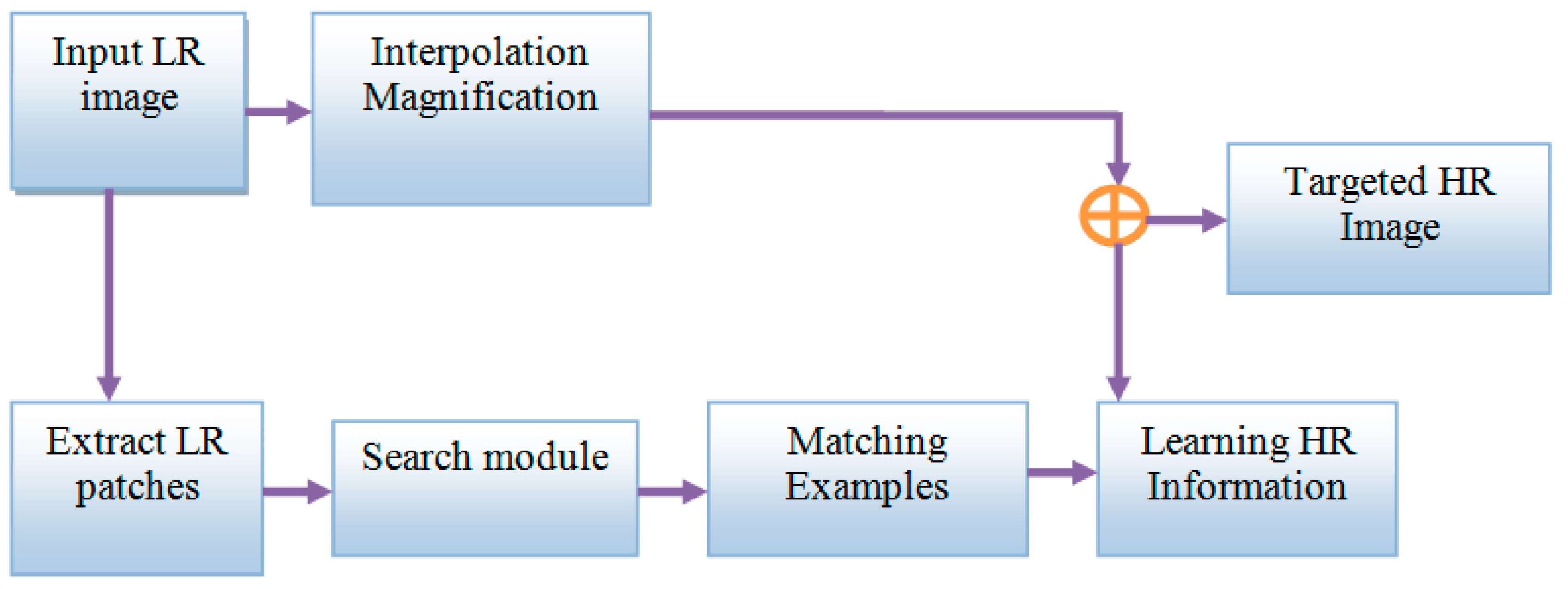
11]. The low-resolution interpolated image is a blurred image that is deficient in high-frequency information, and it is used as a preliminary estimation of the target HR image. Then, the image will be divided further into non-overlapping image patches that are not separate. The framework uses the generated patches to identify the image, which is most matched by searching a training data set of low-resolution and high-resolution image patches. The selected high-resolution image is generated to study high-resolution information. Finally, the trained high-resolution image and the interpolated images are combined to estimate the high-resolution target image. The embedded space is learned for producing solutions with representation, distinct solutions for the same functionality, and picking the group of embedding vectors. Therefore, mapping within the embedding spaces is restricted.
Figure 1 demonstrates the block diagram of SR based face hallucination.
The proposed algorithm was employed to discover the non-linear structure in the data. The algorithm was developed under the assumption that any object is “nearly” flat on small scales. The initial object was to map data from one space globally to another space by embedding the locations of the neighbors for each point. For face hallucination, it was about LR and HR face image spaces. The main idea of the proposed methodology was minimizing the reconstruction error of the set of all local neighborhoods in the data set. The reconstruction weights were computed by reducing the reconstruction error using the cost function in Equation (1).
For face hallucination, such reconstruction weights are computed in the LR face image space and then applied to the HR space to reconstruct the HR face image that corresponds to the LR input. The proposed method normally contains the weight matrix
computed from the neighborhood in the same space as the training samples. Similar to LLE, the ALLE (Adaptive locally linear embedding) computes the weights from the space of training samples, which is built adaptively from only the neighborhood of each input, not all training samples. Since some information contained in all training samples can make the optimizer misleading to another optimal value, the threshold of similarity
is defined for building each subspace in Equation (2).
Face image is represented as a column vector of all pixel values. Based on structural similarity, the face image can be synthesized using the linear combination of training objects. In other words, a face image at an unfixed view can also be reconstructed using a linear combination of other objects in the same view aligned as computed using Equation (3).
There is no information to determine the construction coefficients at other views. After obtaining the LR in all views, these LR images are hallucinated to the HR face images of all views using the position-patch methodology. The proposed framework for multi-view face hallucination is to replace the linear combinations in all processes to improve the performance of hallucinating face images in multiple views. The framework means the number of the neighbors can be adapted for each input patches, and this would relieve the deviation from optimal values. The symbols used to construct the proposed framework are demonstrated in
Table 1.
2.2. AIHEM Algorithm
Step 1: Consider a set of starting parameters in incomplete data.
Step 2: (E-step): Using the observed data from the data set approximates the values of the lost data.
Step 3: (M-Step): the complete data generated after the E-step is used for updating the parameters.
Step 4: Iterate Steps 2 and 3 until convergence.
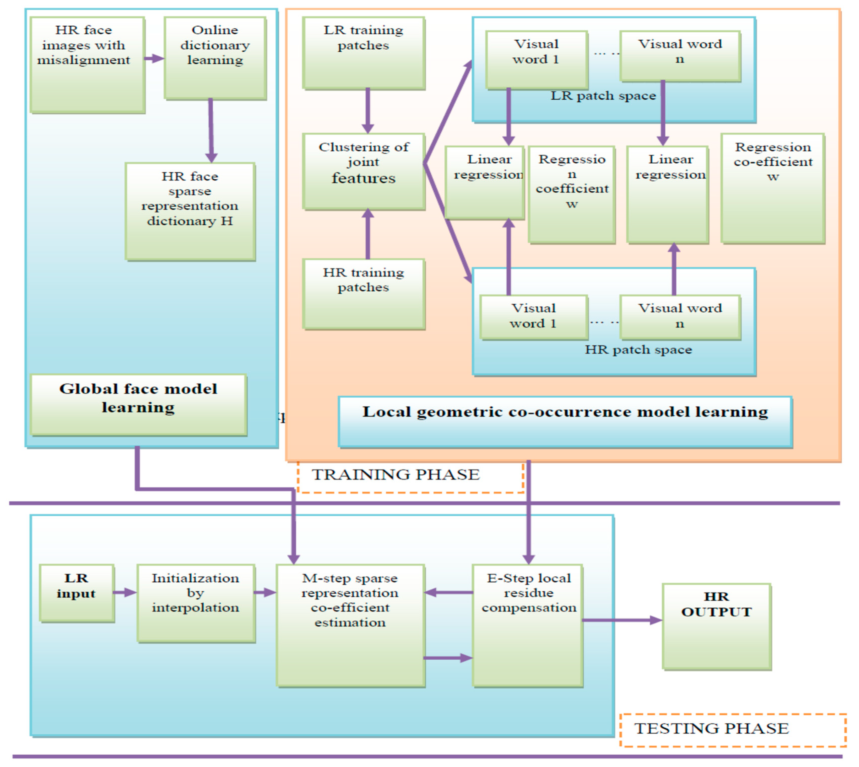
The proposed model consists of 3 phases:
Global face model learning.
Local geometric co-occurrence model learning
Iterative sparse representation optimization.
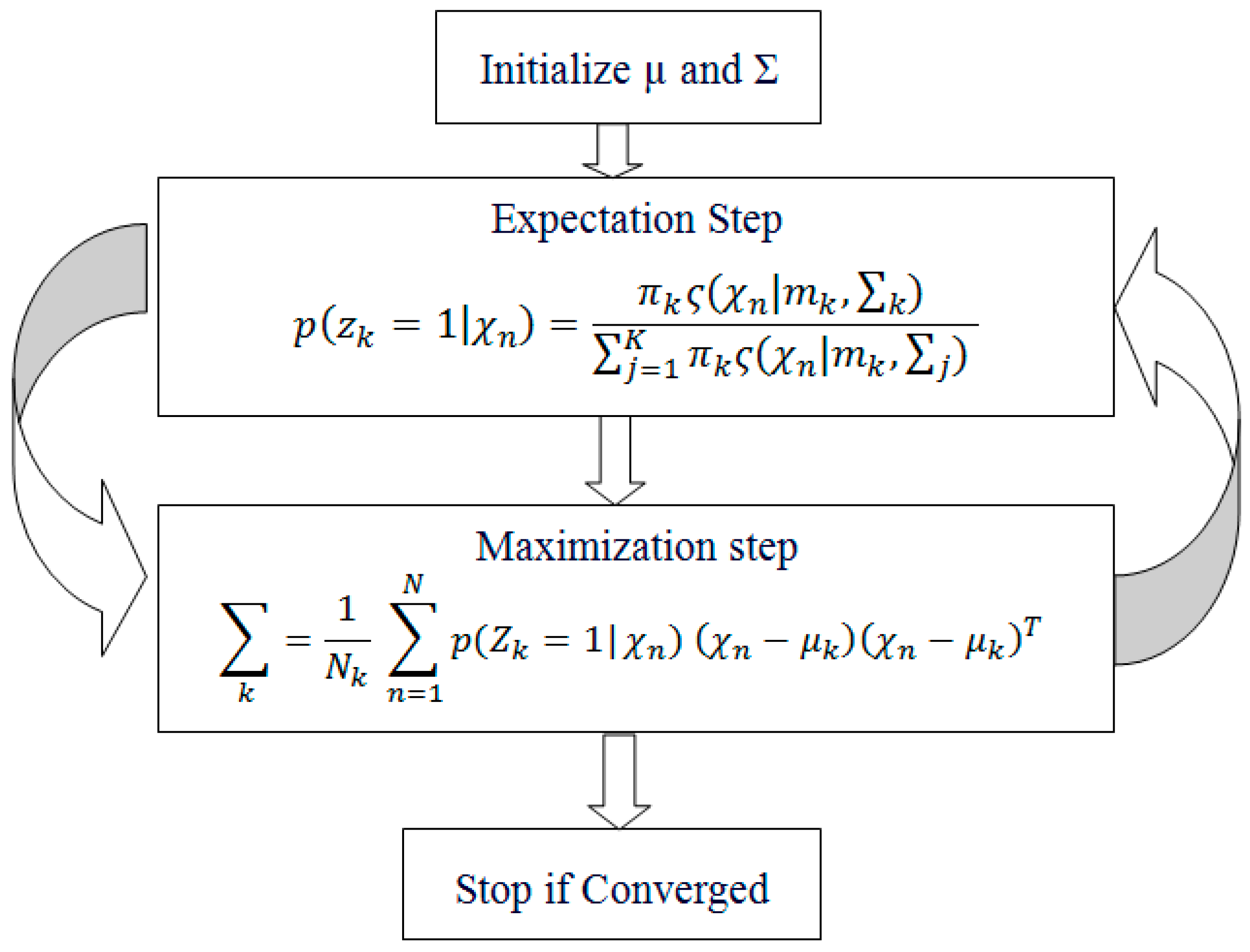
The training phase consists of two parts: The first part is the global face model learning and local geometric co-occurrence model learning. We use a Gaussian mixture model-based estimator for expectation-maximization, as the Gaussian mixture model uses a combination of probability distribution and estimates the mean and standard deviation parameters, as demonstrated in
Figure 2.
Step 1: Consider a set of starting parameters in the incomplete data, with a hypothesis that the observed data is generated from a precise model.
Step 2: E-step—Using the observed data from the data set, approximate the values of the lost data, which are used to update the variables.
Step 3: M-Step—the complete data generated after the E-step is used to update the parameters, i.e., for updating the hypothesis.
Step 4: Checks whether the values are converged, where the concept of convergence is an intuition based on probabilities. When the probability of the variables has a tiny difference, then we say it has converged, i.e., the values are matched. If it is matched, the process stops, otherwise Steps 3 and 4 are iterated until convergence.
2.3. Global Face Model Learning
First, we provide the input HR face images with misalignment and apply the online dictionary to create the dictionary H for the HR face images.
Figure 3 demonstrates the global face model learning. To construct a dictionary to obtain face image “sparsity prior,” face images are preferentially represented by the basis vectors of the same misalignment variation so that the super-resolved HR face images are constrained in a subspace of certain misalignment variation.
HR face images are always highly dimensional (the dimension is 127 × 158 for an HR image and 50 × 62 for an LR image in this paper), and the training set needs to be large enough for training the redundant dictionary. However, in practical applications, the computational complexity of the sparse problem is very high with an extensive dictionary. Generally speaking, the computational cost is proportional to the size of the dictionary H, i.e., a size of ¼ nm, where n is the dimension of the HR face image, and m is the number of basis vectors in the dictionary. Since the solutions are usually an iterative method dealing with a large dictionary matrix, the storage requirements and computational cost are significant. In our case, if all images with different misalignment variations were selected to compose a dictionary, it would be difficult to solve the super-resolution problem. Thus, we considered dictionary learning to compress a dictionary to reduce the operational burden. Batch-based methods have problems dealing with an extensive training matrix effectively. This paper employed an online dictionary learning method to process the images, one at a time, with low memory consumption and lower computational costs. The number of basis vectors in the dictionary was 1024. The following steps were required to perform online dictionary learning.
Assume the training set, such as the first dictionary and number of iterations.
Reset the past information.
Find the sparse coding using LARS (least angle regression coefficient).
Here is dictionary coefficient
is Lagrange’s multiplier.
is an Original data.
is the created dictionary.
Suffix 2 is a normalization factor.
Compute the learned dictionary,
Here i is loop iteration.
Get the updated dictionary.
2.4. Local Geometric Co-Occurrence Model Learning
The following steps are required to perform the local geometric co-occurrence model learning:
Consider the training set LR and HR face residue.
Get the local geometric feature representation for each patch.
Connect the HR and the corresponding LR geometric feature vectors for jointly learning the HR and LR visual vocabularies.
Apply the affinity propagation clustering algorithm.
All data points are considered simultaneously as candidate cluster centers.
Messages are transmitted between the data points until an appropriate set of cluster centers and corresponding clusters emerge.
The number of clusters also depends on a prior specification of how preferable each data point is as a cluster center.
Consider all data points that have equal potential to be the cluster centers, so the preferences of all data points are set to the same value that can be controlled to produce different numbers of clusters.
In the testing phase, there were three steps to be followed. In the first step, we chose the LR image. Then, the initialization and the optimization process were performed. The LR image was given as input and it was initialized by interpolation. That image was compared to the global face image and processed to the M-step. Hence, the initialized image was compared to the local geometric co-occurrence model image, where that image was a process in the E-Step. Finally, the M-step and the E-step image was optimized. The geometrical feature that was defined in this section represented the high-frequency structures that are due to various intensity changes.
2.5. Demonstration of Execution Steps of the Proposed Method
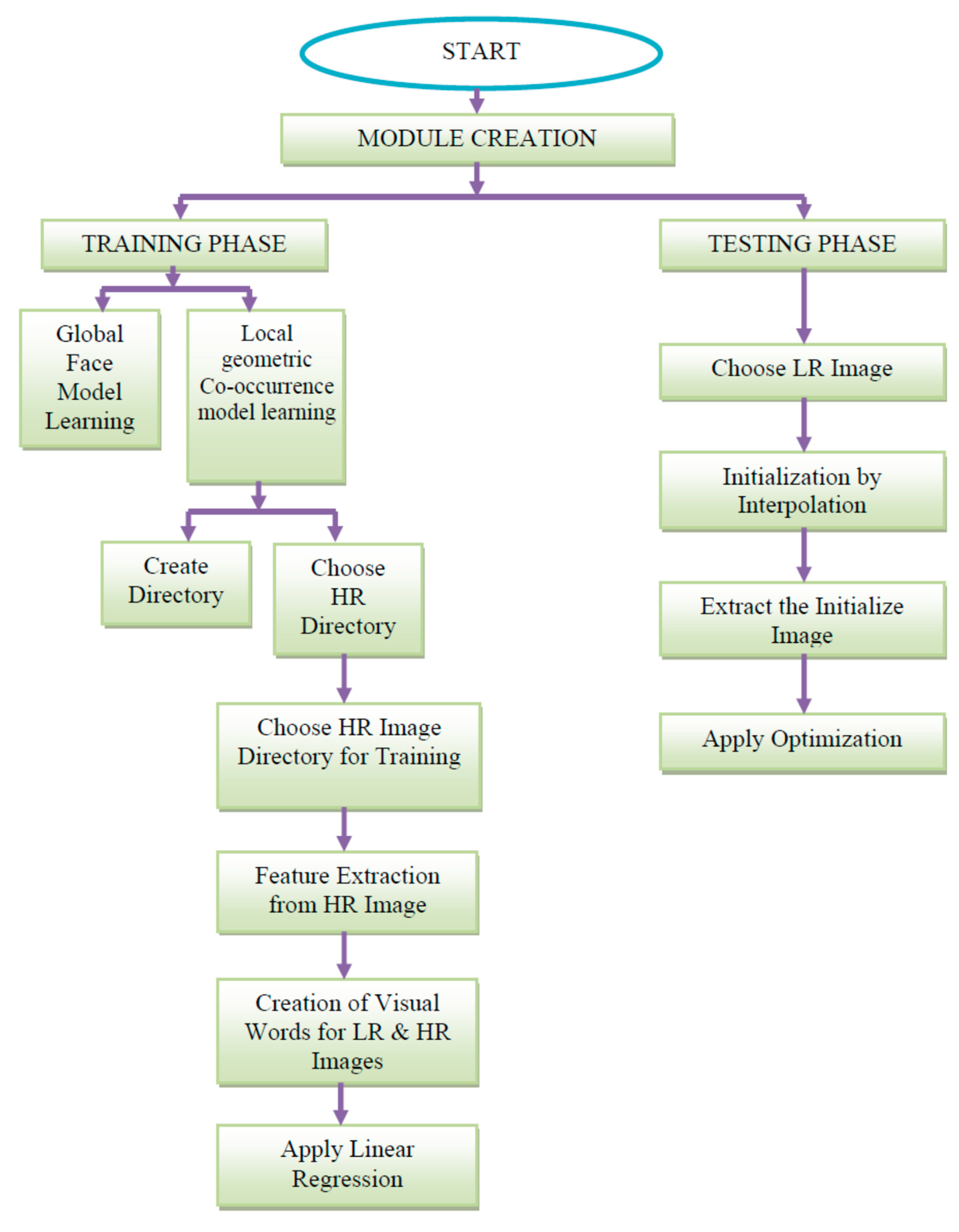
Figure 4 demonstrates the execution steps for the proposed method.
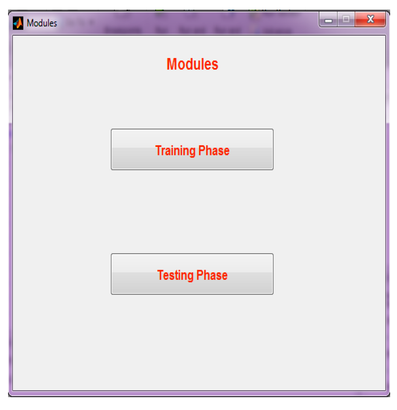
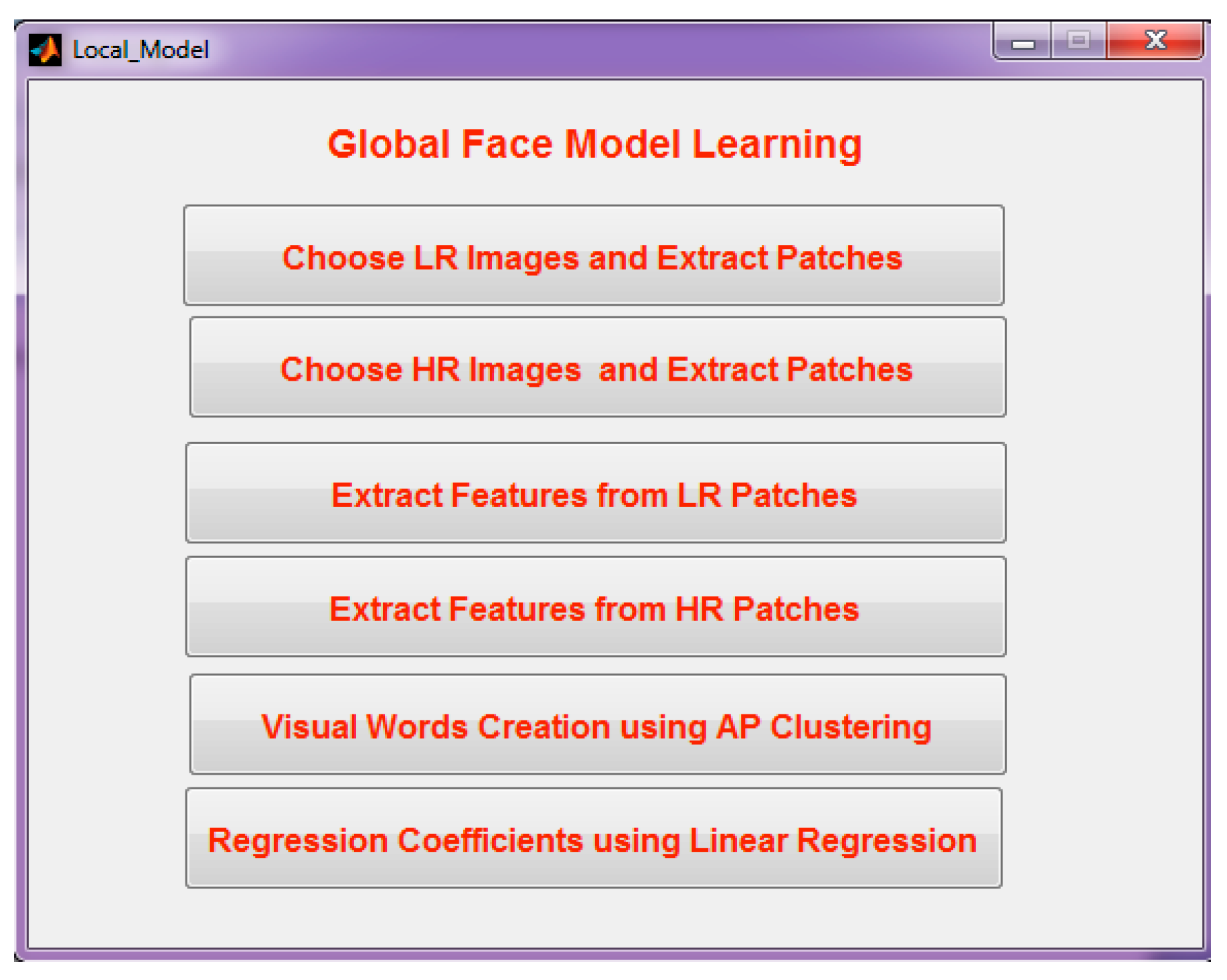
Step 1: The modules are selected from the graphic user interface. In the training phase, there is global face model learning and local geometric co-occurrence model learning. Here, two modules can be selected. The first module is the training phase, and the second module is the testing phase.
Figure 5 illustrates the GUI (Graphical User Interface) of Module Selection.
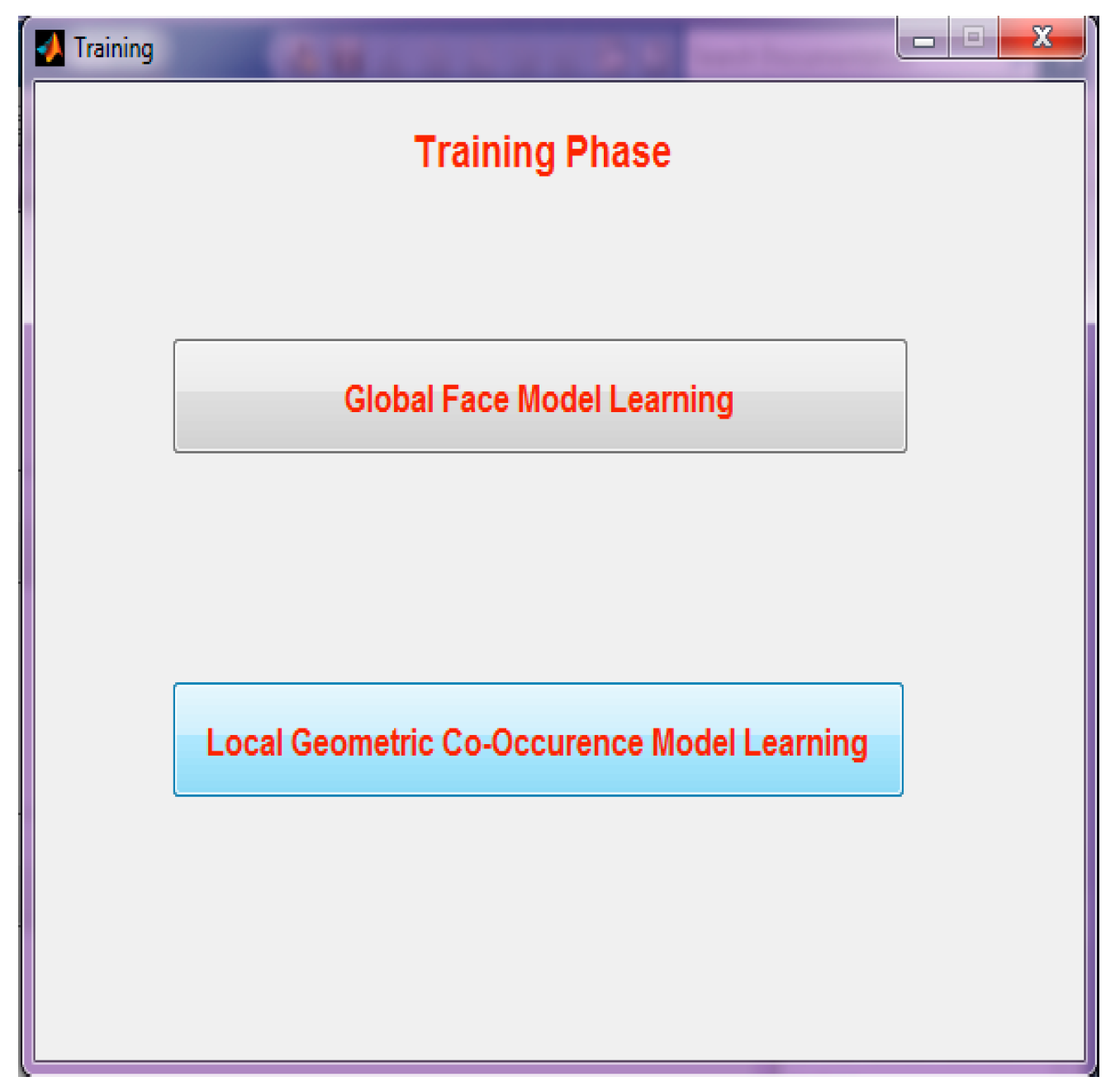
Step 2: Selection of training phase, the second page opens, which is the GUI of the Training Phase, which contains global face model learning and local geometric co-occurrence model learning.
Figure 6 demonstrates the GUI of the training phase.
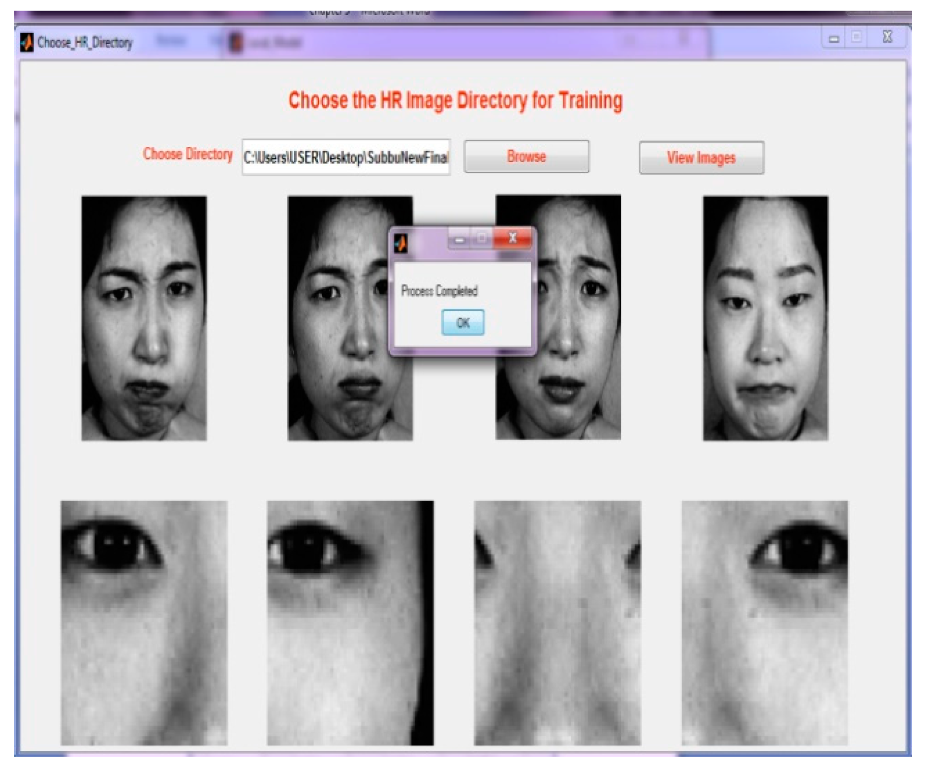
Step 3: Selection of the global face model learning. Two directories can be chosen as the high-resolution directory, and they create the dictionary.
Figure 7 illustrates the GUI of the global face model learning phase.
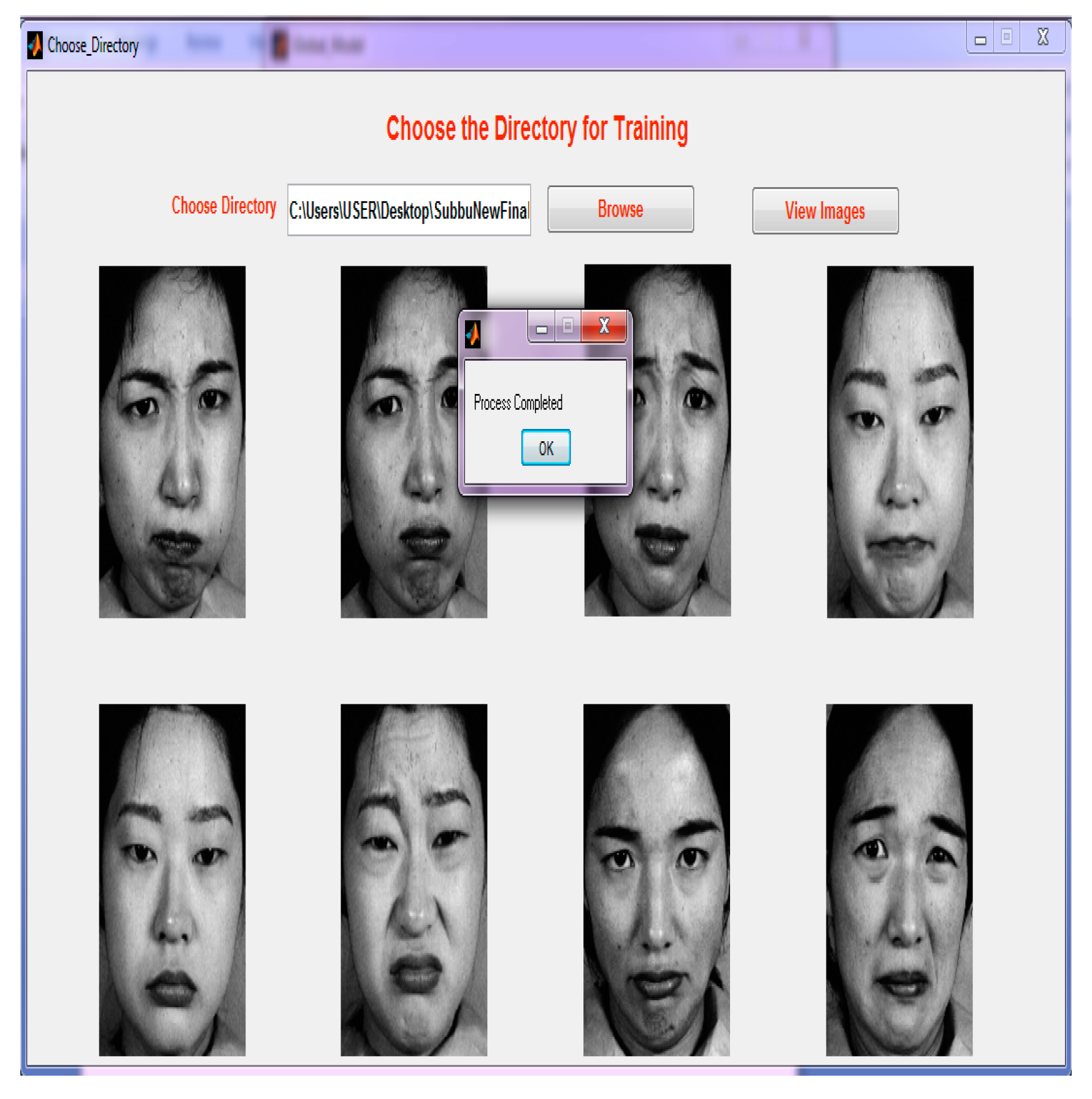
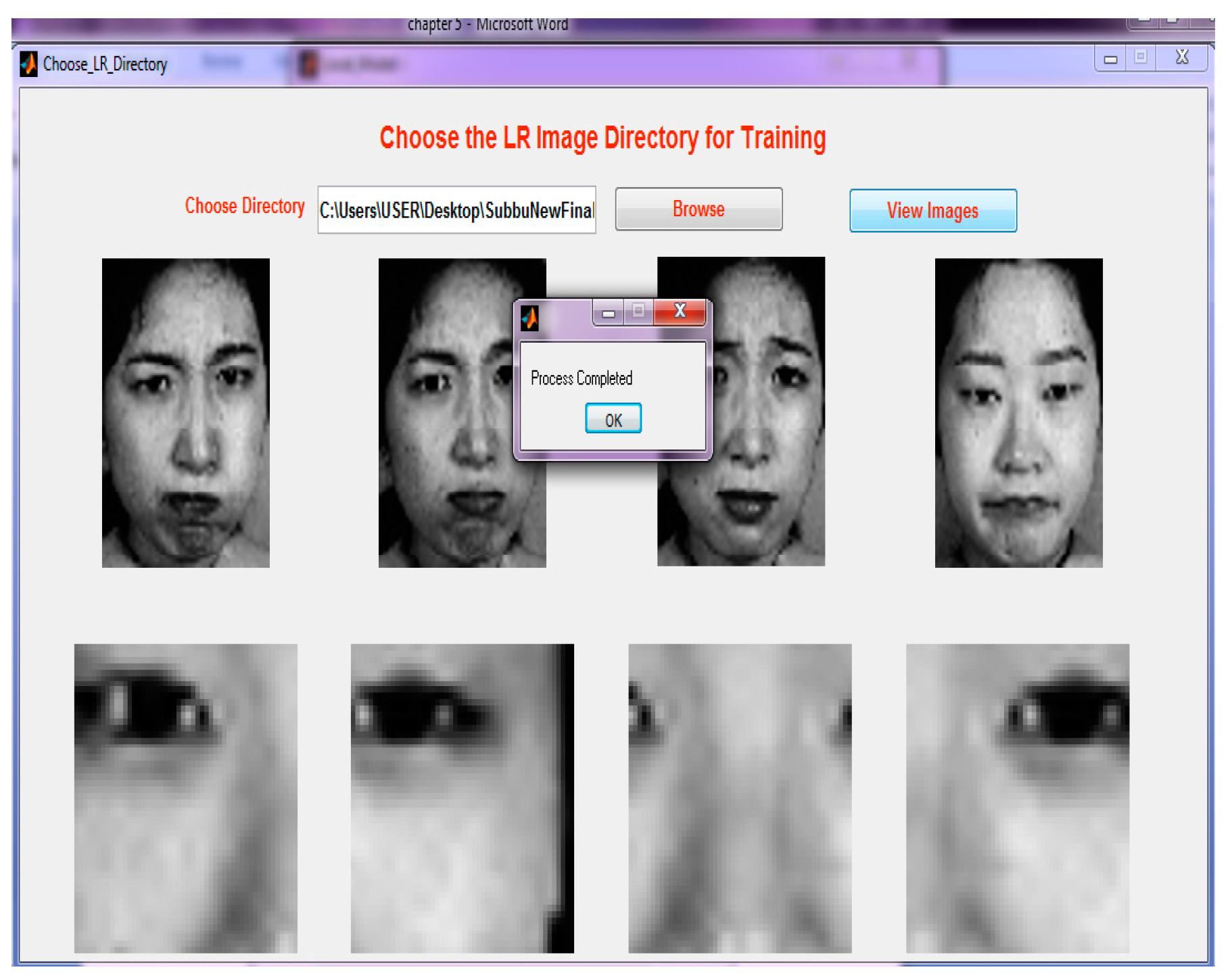
Step 4: Choosing a directory for training the GUI for every image. Three poses are created so that it will be easy to compare the images with the testing phase.
Figure 8 illustrates the GUI for directory selection.
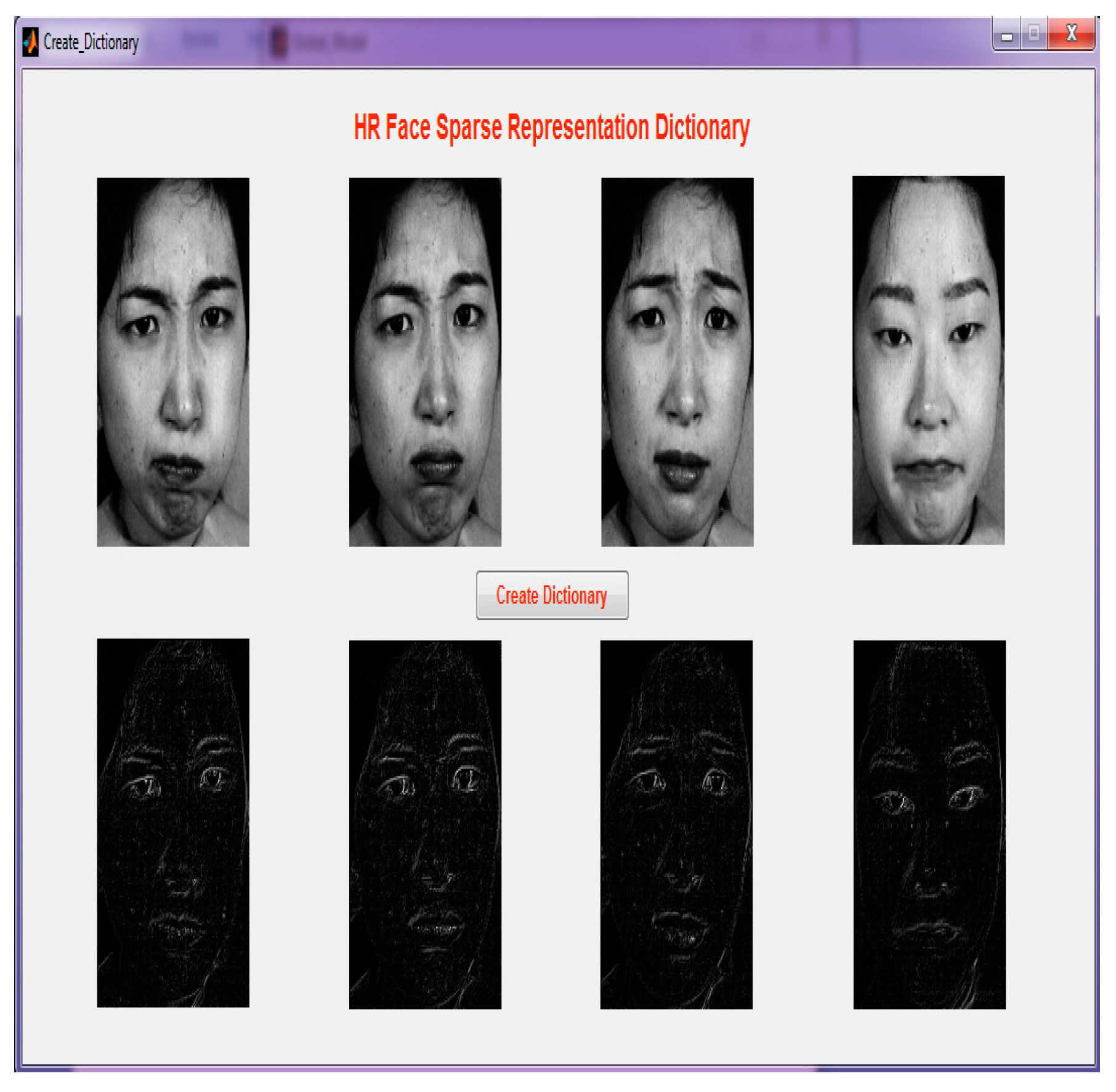
Step 5: All images with different misalignment variations are selected to compose a dictionary. This output shows that the dictionaries are created for each directory using online dictionary learning.
Figure 9 demonstrates the GUI of the HR face sparse representation dictionary.
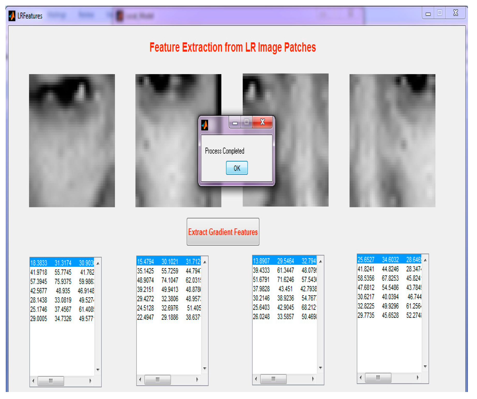
Step 6: Steps in local geometric co-occurrence model learning. The first step chooses the LR images and extracts features from the LR patches, and the second step chooses the HR images and extracts the features of the HR patches.
Figure 10 illustrates the GUI of global face model learning.
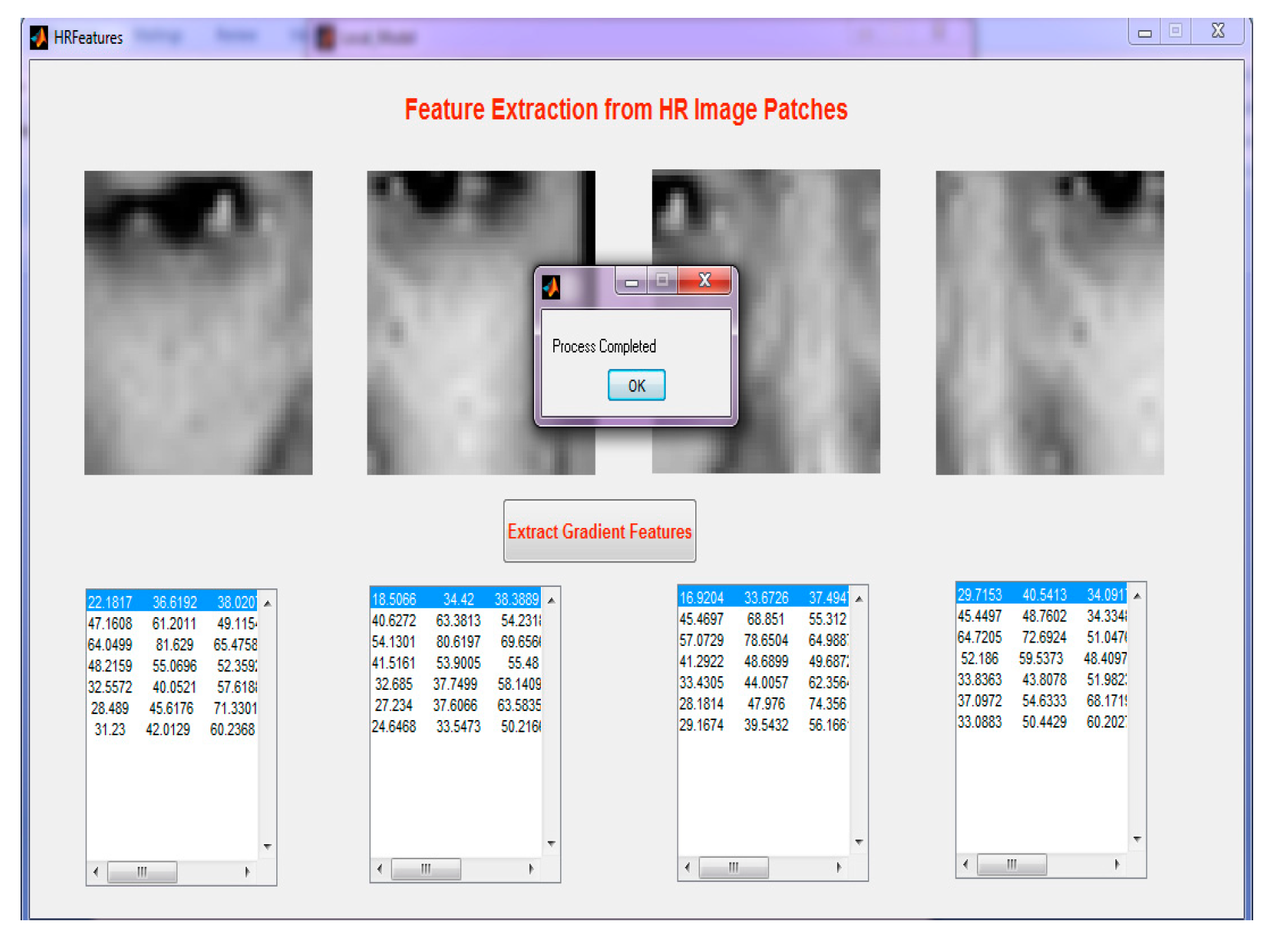
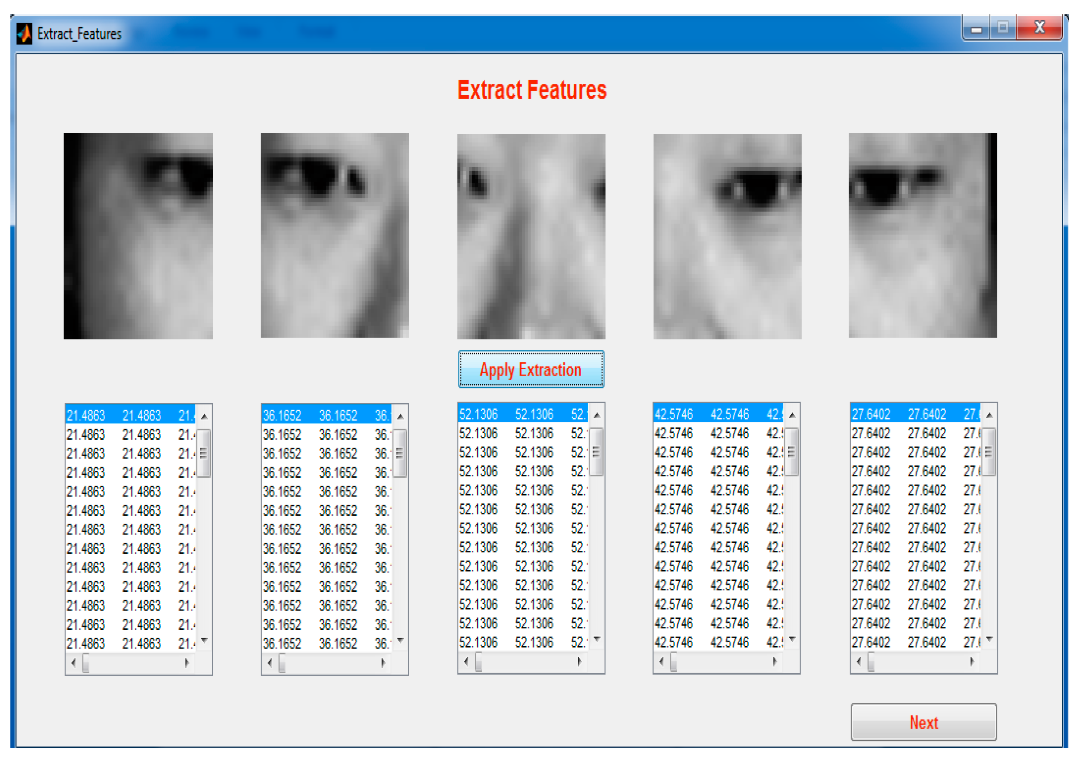
Step 7: The given global face input image is divided into LR (Low resolution) and HR (High Resolution) patches that include individual parts such as the eye and nose region.
Figure 11 demonstrates the selection of the LR image.
Figure 12 illustrates feature extraction from the LR image.
Figure 13 demonstrates the selection of the HR image.
Figure 14 illustrates feature extraction from the HR Image.
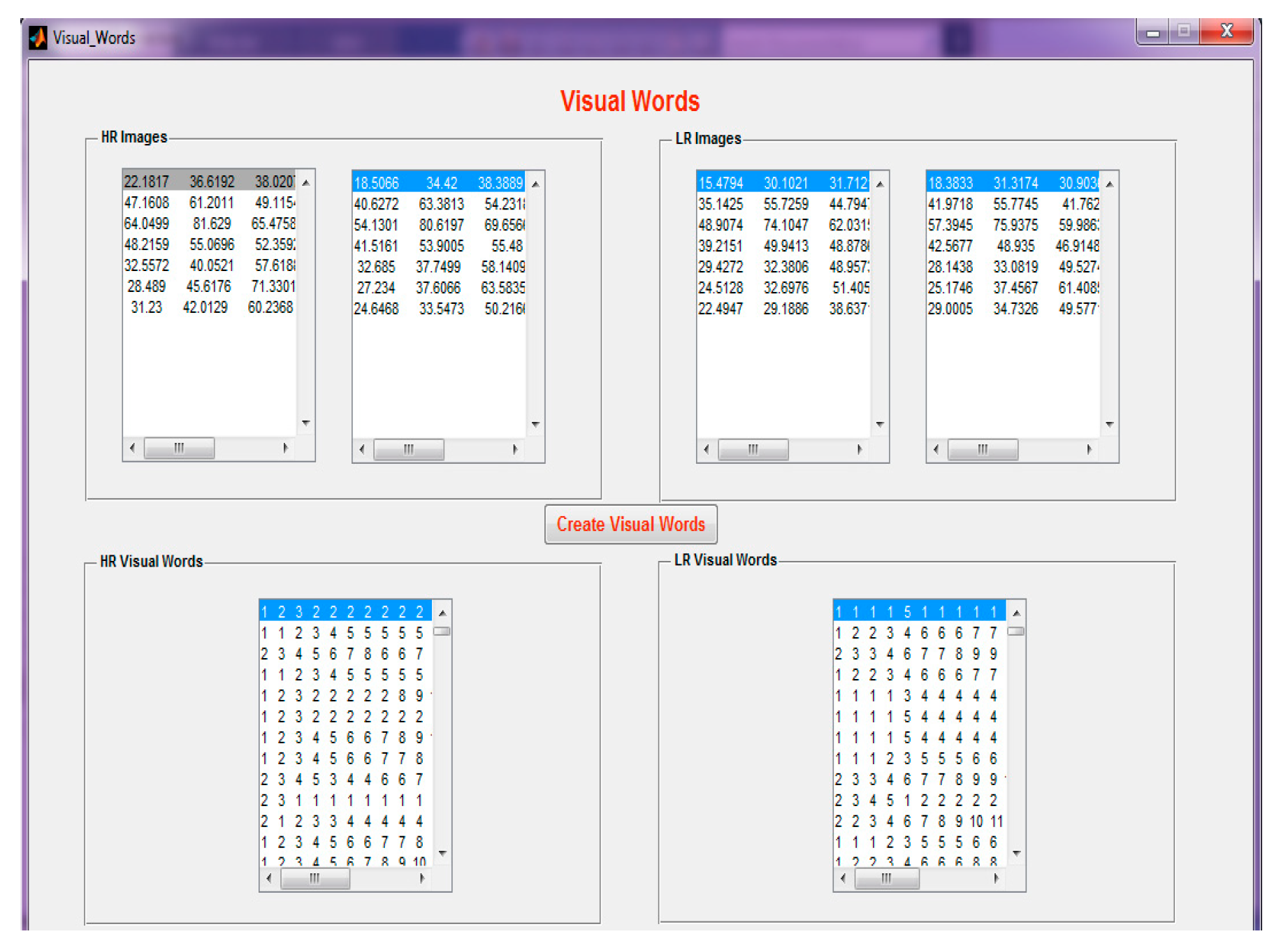
Step 8: On extraction of the HR and LR features from the input image, visual words are created for both the LR and HR, separately.
Figure 15 demonstrates the creation of visual words.
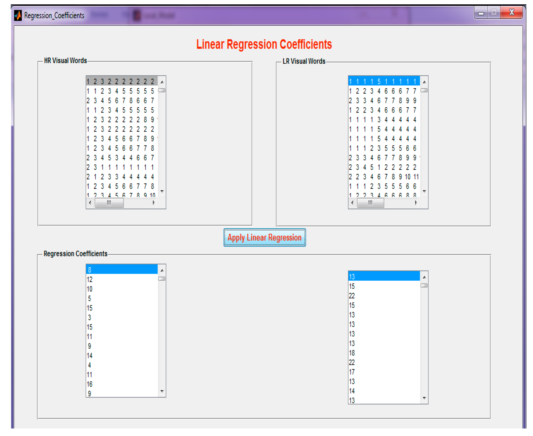
Step 9: Applying linear regression to the HR and LR visual words, the regression coefficients are determined. The regression coefficients are calculated by finding the mean value of the RGB (Red-Green-Blue) of the HR and LR image gradient features.
Figure 16 demonstrates the application of linear regression on visual words.
Testing Phase:
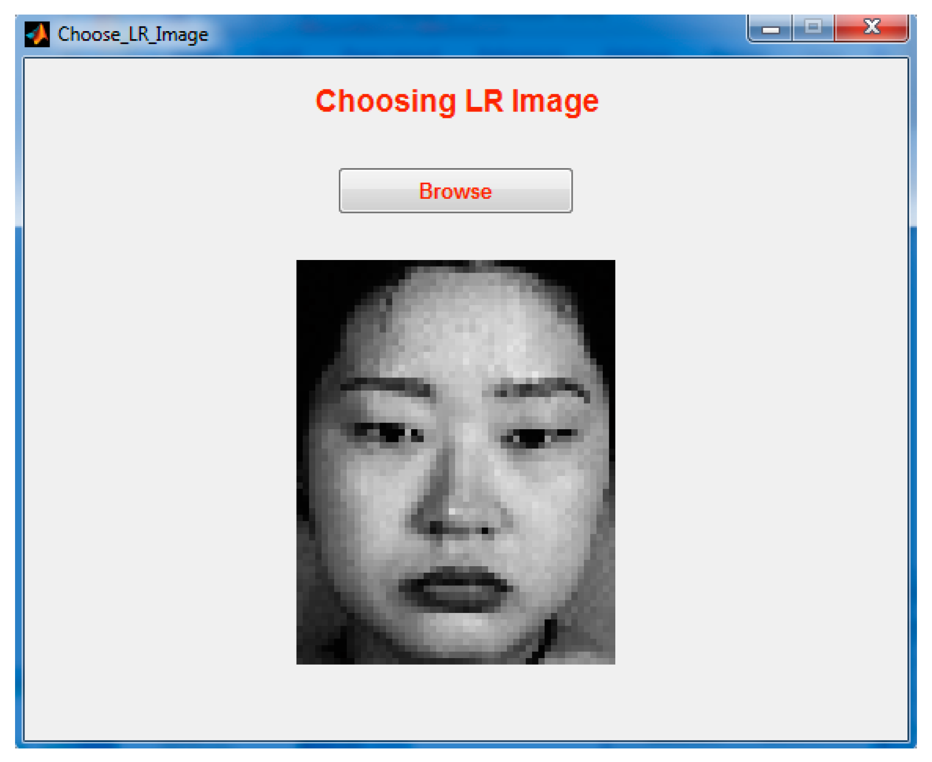
Step 1: Choosing an LR Image.
Figure 17 demonstrates choosing the LR image from the directory.
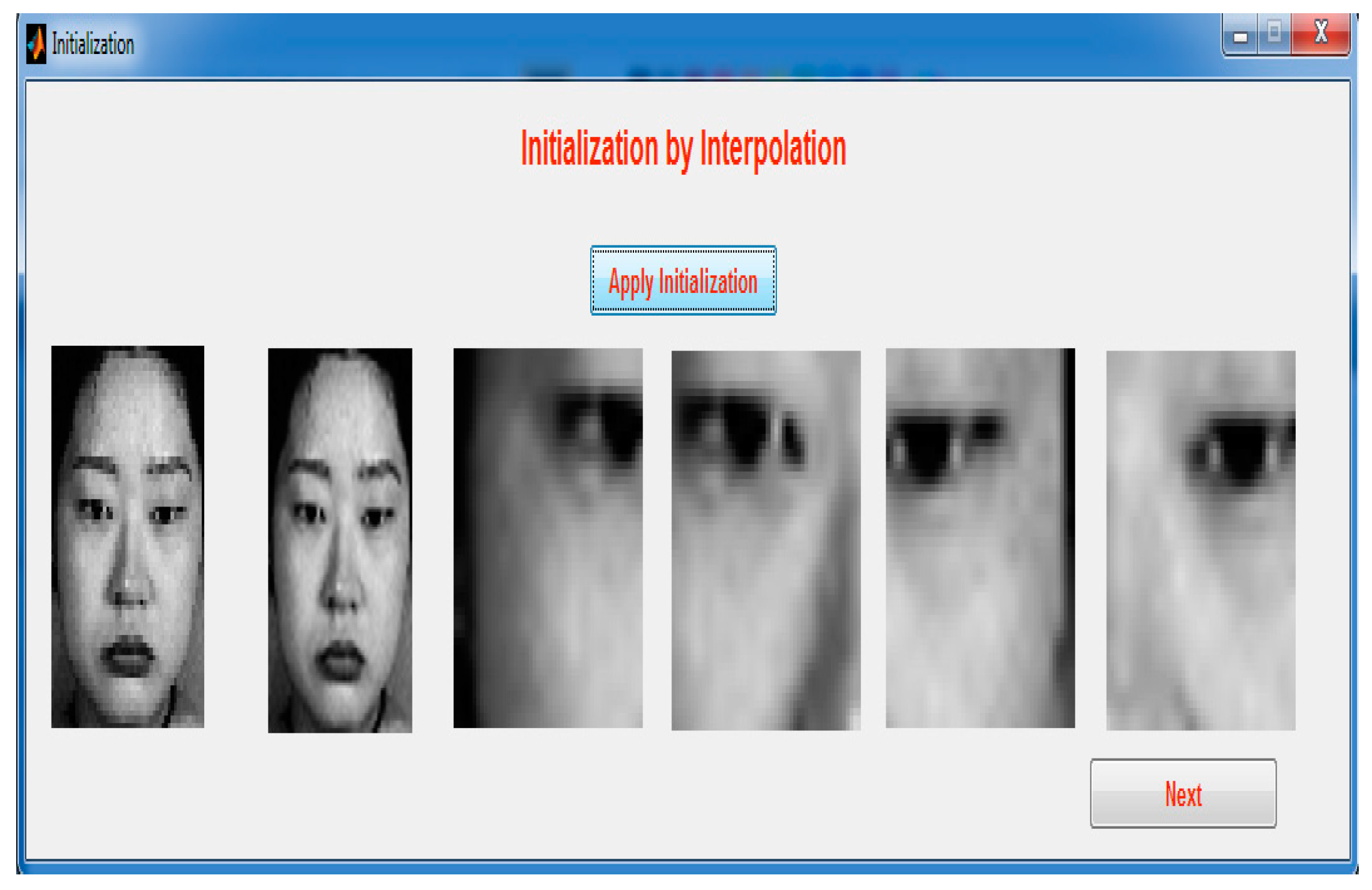
Step 2: The LR image should be applied for initialization by interpolation for resizing the LR image, which is easy to compute using the global face model.
Figure 18 demonstrates initialization for interpolation.
Figure 19 illustrates applying interpolation. After applying the initialization, the same LR image is split into patches.
Figure 20 demonstrates initial image extraction. The LR image should extract the features and give the gradient of the features. Then, the feature is compared to the local geometric co-occurrence model of the training phase.
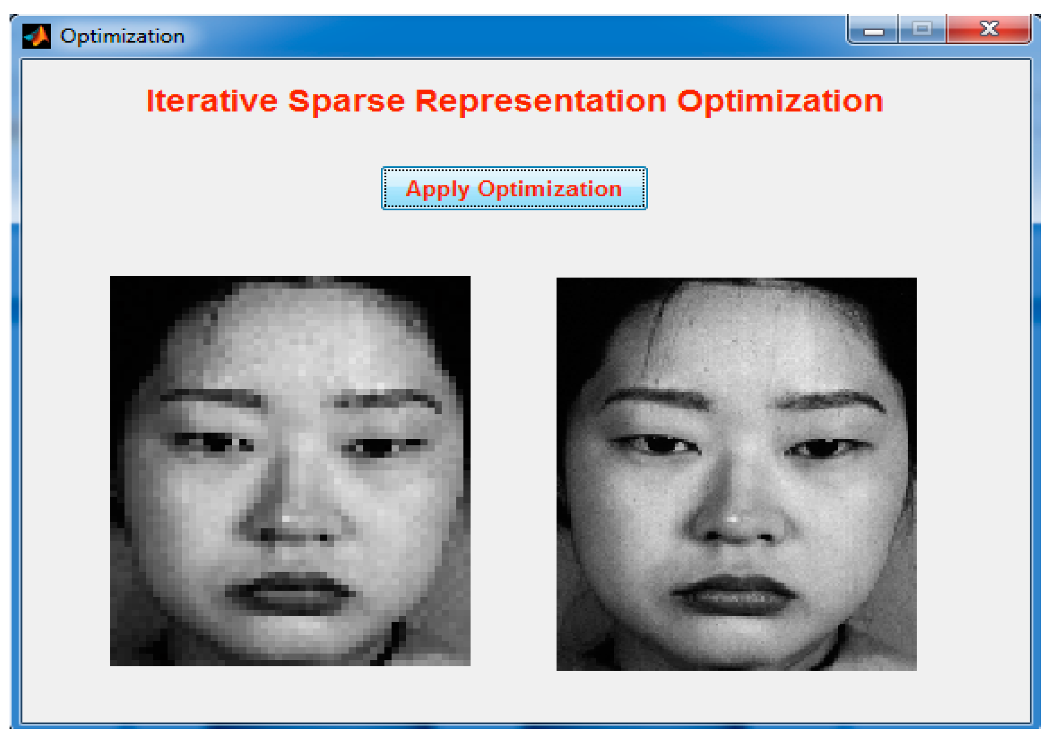
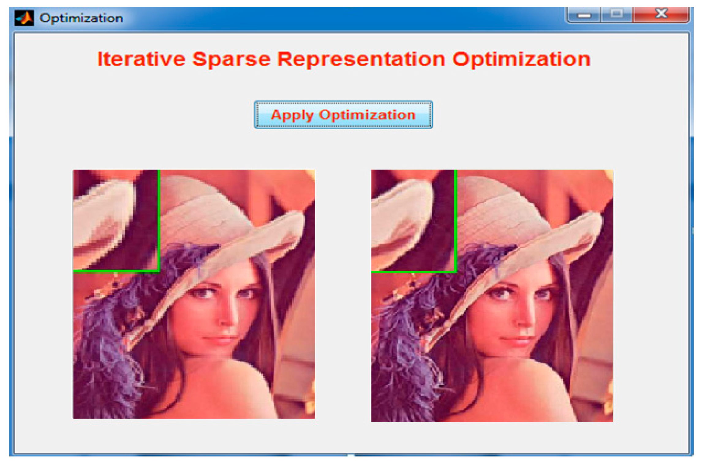
Step 3: Optimization.
The input LR image is initialized, and then the E-step is applied. In this step, the LR image is given as the input and it is initialized by interpolation. The image is compared to the global face image, and then it is processed to the M-step. Hence, the initialized image is compared to the local geometric co-occurrence model image, and that image is processed to the E-Step. Finally, the M-step and the E-step image is optimized.
Figure 21 demonstrates the optimized image of the input LR image. The technique works perfectly with an RGB image like the black and white image shown in
Figure 22.
This method consists of training testing phases. The training phase consists of two parts. The first part is global face sparse representation learning in which an online dictionary is used to learn the face prototype dictionary. The second part is a local geometric co-occurrence before learning, where we jointly clustered the HR and LR image residue patches and learned the regression coefficients from the LR to HR visual vocabulary.
In the testing phase, when the LR face image is presented, an initial image was generated by simple interpolation. An iterative sparse representation model using the learned dictionary was proposed to generate an HR image. The representation coefficients were iteratively optimized using the EM algorithm, in which local residue compensated to the global face using linear interpolation.
The training phase consisted of two parts. The first part was the global face model learning, and the second was the local geometric co-occurrence model learning. In global face model learning, two directories choose the high-resolution directory and create the dictionary. The images are selected from the directory for training. In the database for every image, three poses were created so that it would be easy to compare the images with the testing phase. All images with different misalignment variations were selected to compose a dictionary. This output showed that dictionaries were created for each directory using online dictionary learning. In the local geometric co-occurrence model learning, the first step was to choose the LR images and extract the features from the LR patches. The second step involved choosing the HR images and extracting the features of the HR patches.
The given global face input image was split into LR (low-resolution) patches that included unique parts such as the eye and nose region. It showed the features of the LR image and that the images should extract the gradient features. The given global face input image was split into HR (high-resolution) patches that included unique parts such as the eye and nose region. It showed the features of the HR image and that images should be extracted from the gradient features. The visual word was the collection of all local geometric features. The visual words were created for both HR and LR images separately. HR and corresponding LR geometric features were joined together for learning the HR and LR visual words. Regression coefficients were determined by applying linear regression to the HR and LR visual words. The regression coefficients were calculated by finding the mean value of the HR and LR image gradient features. In the testing phase, the global and local geometric features are involved. During the testing phase, three steps should be followed. The first step is choosing the LR image. Then the initialization and the optimization processes are performed.
The LR image should be applied for the initialization by interpolation, for resizing the LR image. It is used to compute the global face model. After applying the initialization, that same LR image is split into patches. The LR image should be extracted from the features, and it gives the gradient of the features. Then the feature is compared to the local geometric co-occurrence model of the training phase. The input LR image is initialized, and then the E-step is applied. In this step, the LR image is given as input, and that is initialized by interpolation. Then the image is compared to the global face image, after that the image is processed to the M-step. Hence, the initialized image is compared to the local geometric co-occurrence model image, where that image is processed to the E-Step. Finally, the M-step and the E-step image are optimized. The Kalman filter is used during the image optimization process. It is very effective in performing computational operations with linear filter modeling. It can produce an estimation of the current states of the system to remove the noise in the image. The main goal of utilizing the Kalman filter is to predict the position of a particular area of an image to be evaluated during the image optimization process. The expected position measures the prediction for the identifying area and it is identified using the variance and the confidence level. Building robust dictionaries is required to recover the high-resolution images and remove the dark regions of the images.
3. Performance Evaluation
The implementation requires an i3 processor with a 4GB RAM on MATLAB R2018b using the Windows 7 operating system. The proposed method was compared to related methods, e.g., SRGAN [
28], TRNR [
27], and LSR [
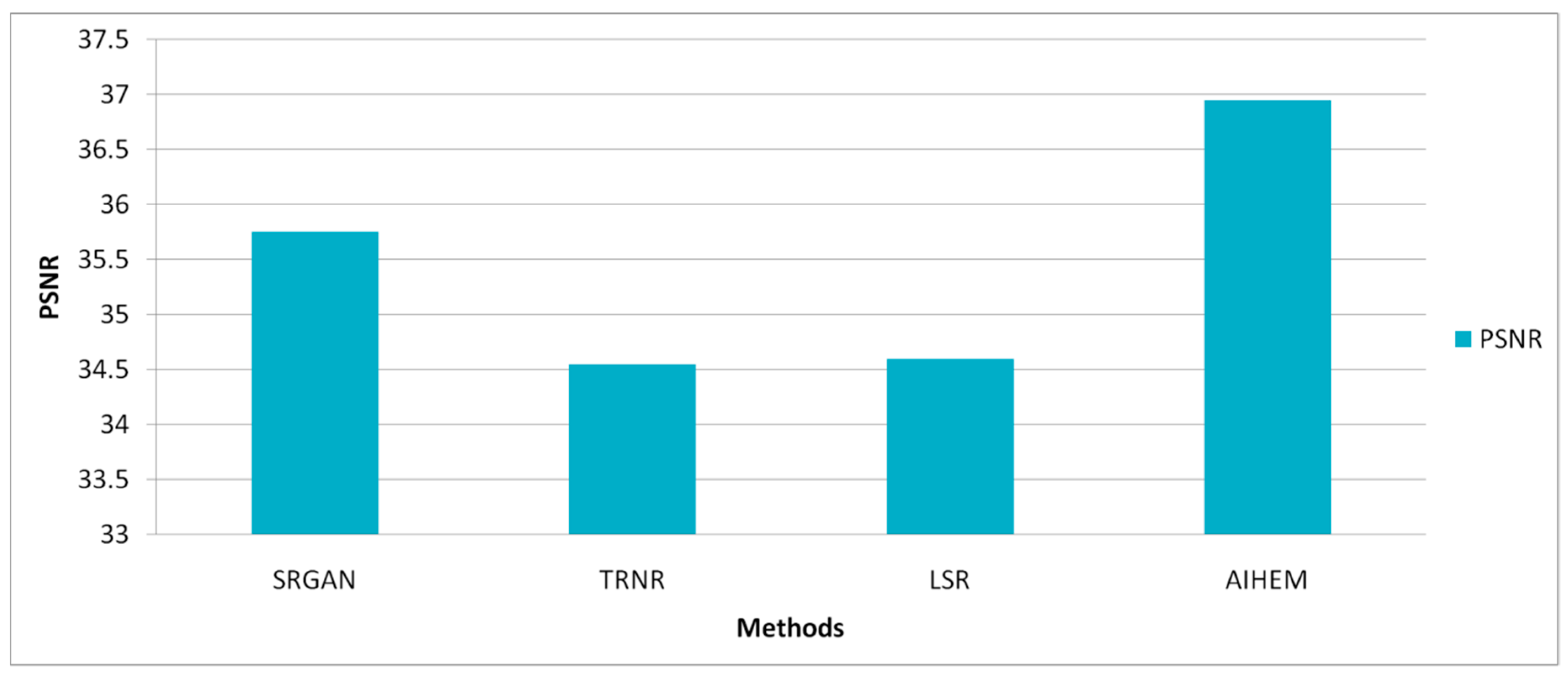
26]. Here, the time taken analysis is denoted by the training phase image value. Each individual has five different views (left, right, up, down, and frontal views) under the same light conditions. These face images were aligned manually using the locations of three points: centers of the left and right eyeballs and the center of the mouth. Some aligned face images were cropped to 32 × 24 pixels for low-resolution face images, and to 128 × 96 pixels for high resolution face images. Based on the same training sets, the proposed method was compared to related methods. Each input face image was generated into five different outputs of LR, synthesized LR face images, and HR face images according to the framework.
Table 2 demonstrates the list of PSNR values of the hallucinated image with an input face image on the frontal view. The value of
K is 100 and
= 0.1.
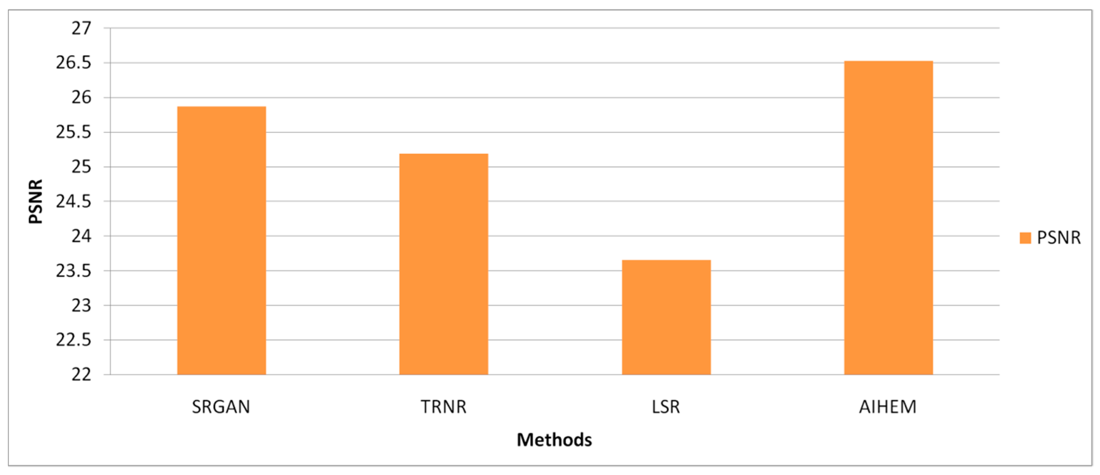
Table 3 demonstrates the list of PSNR values of the hallucinated image with an input face image on the up view. The value of
K was 200 and
= 0.2.
Table 4 demonstrates the list of PSNR values of the hallucinated image with an input face image on the down view. The value of
K was 200 and
= 0.2.
Table 5 demonstrates the list of PSNR values of the hallucinated image with an input face image on the left view. The value of
K was 200 and
= 0.2.
Table 6 demonstrates the list of PSNR values of the hallucinated image with an input face image on the right view. The value of
K was 200 and
= 0.2. The threshold of similarity was used to find the similarity within a collection of objects. It contained several factors to determine scalability and minimize computational cost. In the testing phase, it generated the low-resolution input images to high-resolution images. The semantic class of the image was essential for solving within the inherent class to achieve the improved result. In-depth features can be implemented to increase the accuracy.
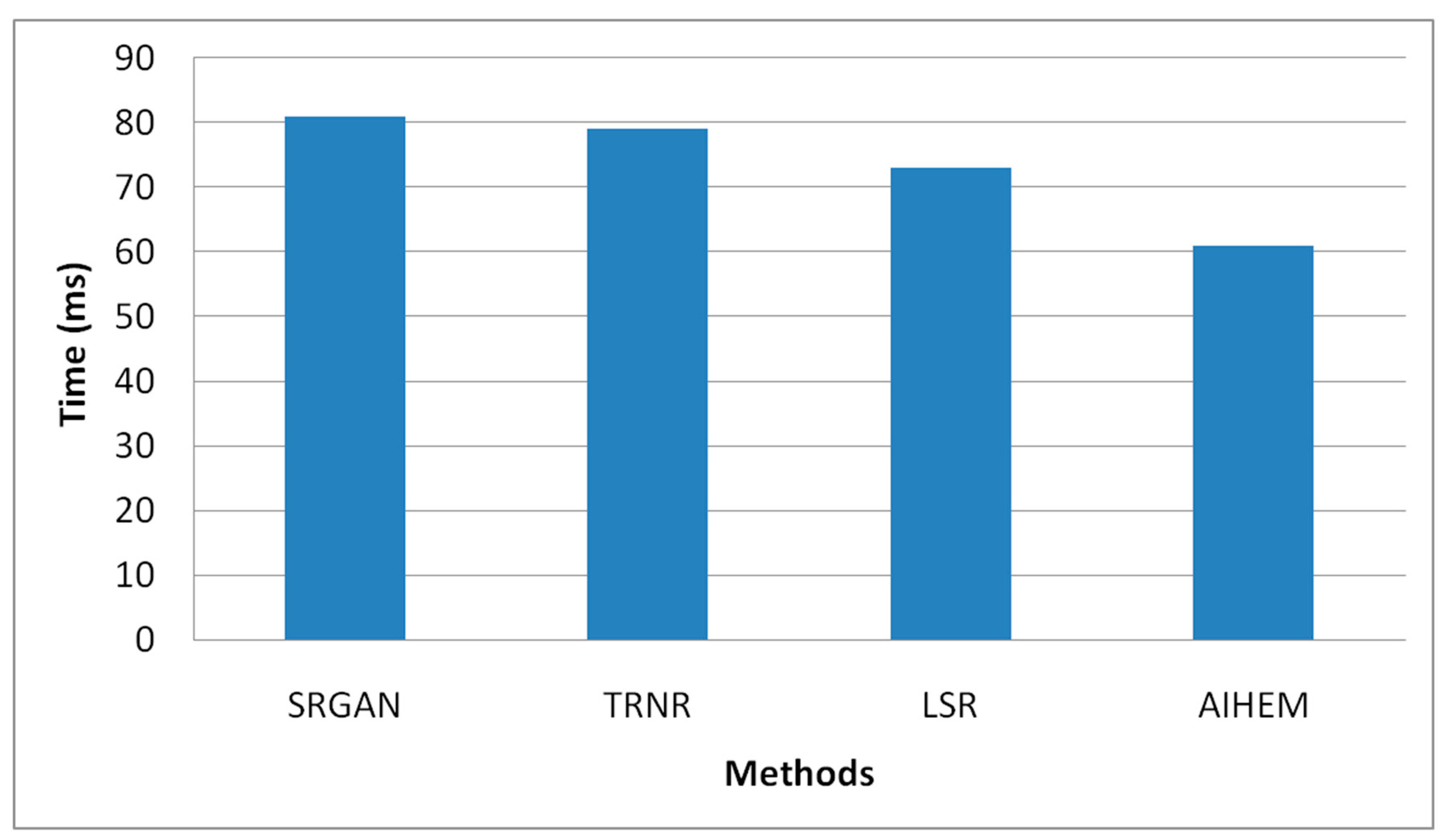
In
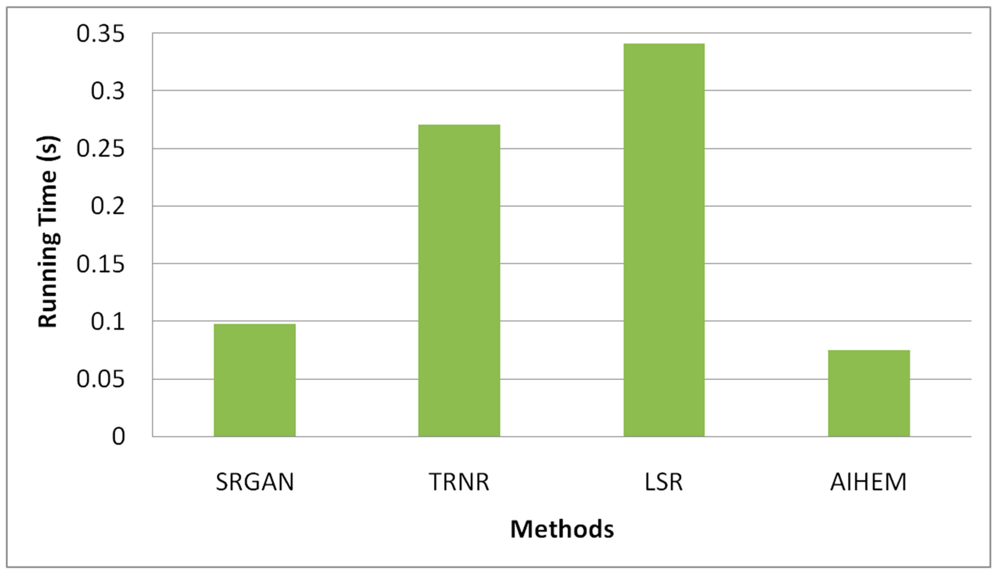
Figure 23, the accuracy is high because all images are performed by the training phase so that there is no error rate. The precision rate and recall rates are also equally high. Running time for evaluating the efficiency of the proposed methodology was compared to the related methodologies. The proposed method ran faster than the related methods because of its fast optimization techniques.
Figure 24 demonstrates the running time. The experimental results showed the higher quality of reconstructed images of the proposed framework over the enhanced methods with interpolation. High-resolution face images of five different views were generated from a single low-resolution face image. According to the experimental results, the reconstructed image was more accurate if the view of the input image was the same as that of the output. Particularly, frontal, up, and down views achieved better estimations than others. The results of the proposed method showed superior reconstruction quality of the HR face image over other related methods in both visualization and PSNR values.
The proposed AIHEM methodology was based on the EM algorithm, which is non-deterministic; thus, the performance evaluation was performed multiple times using standard deviation values. The standard deviation value was measured to obtain the PSNR value for the proposed method, as compared to the related methods. The performance results may vary in several iterations of continued evaluation, and the results are shown in
Figure 25 and
Figure 26. The results showed a standard deviation of 10 and a standard deviation of 100, respectively.
The proposed method was a very effective technique and required fewer computational resources, so the processing was easy to produce the solutions for the optimization problems. It is useful to recognize and tune the data with predictable output. The performance improved compared to the related methods, and it was straightforward to train the dataset. The measurement of accuracy is an integral part of image classification when validating the proposed work. The vectors were used to extract the features to achieve the highest amount of accuracy. The iteration model was used to classify the image based on the similarity parameter from a pixel by pixel.
The computational complexity of the proposed system was analyzed using the big oh notation , for the face hallucination methodology. The pre-processing and alignment methods were crucial to reducing computational complexity. The performance was analyzed using a threshold-based similarity that was 35 times faster than the other methods. The running time for the image in the testing phase was 13.5 s while using the proposed mechanism. The proposed method had a considerable development that attained a steady performance at a size of pixel frame. Whenever the size increases, the running time will also increase. To minimize the computational complexity of the proposed algorithm, we maintained the size of the pixel frame as pixels for performance evaluation.

 ,
, 


