The Influence of Energy Certification on Housing Sales Prices in the Province of Alicante (Spain)

 ,
,  , and
, and
Abstract
:1. Introduction
2. Materials and Methods
2.1. Population and Sample
2.2. Sources of Information
2.3. Data
2.4. Descriptive Statistics
2.5. Methodology
3. Results
3.1. One-Way Analysis of Variance (ANOVA)
3.2. Regression Analysis
4. Discussion
5. Conclusions
- -
- First, real estate sellers and owners who do not publish energy qualifications offer their homes at prices that are similar to those having high qualifications.
- -
- Second, there is the lack of sanctions placed by the public administration on companies, owners and real estate portals that do not publish the energy qualifications of the housing that is for sale or rent, motivating owners to not publish the letter and generating distorted asking prices for the housing. Therefore, it is important for the administration to closely supervise compliance with regulations and assign the necessary resources to local authorities to ensure said compliance, and if needed, to impose sanctions.
- -
- Third, owners are not interested in improving energy qualifications, since, according to [71,72] there is no compensation for the additional investment needed to improve this qualification. And fourth and finally, the current regulations for housing only require that these homes obtain energy qualification if they are going to sell, rent or publish. However, there is no obligation to obtain a minimum qualification, so the improved energy performance of the homes is not encouraged [73,74].
- -
- Fifth and finally, society’s perception of EPC is negative, as revealed by several studies relying on surveys completed by professional real estate agents [74,75] or energy certifiers [73]. Regardless, these studies suggest that the main criteria used to select a home is price and location [74,75,76].
Author Contributions
Funding
Acknowledgments
Conflicts of Interest
Appendix A

| Block | Indicator | España | Alicante | Source |
|---|---|---|---|---|
| Use of the housing (2011) | Main housing | 18,083,692 (71.7%) | 738,367 (58.0%) | [36] |
| Secondary housing | 3,681,565 (14.6%) | 326,705 (25.6%) | ||
| Empty housing | 3,443,365 (13.7%) | 209,024 (16.4%) | ||
| Tenancy regime (2011) | Ownership | 14,274,987 (85.4%) | 613,626 (88.6%) | [36] |
| Rental | 2,438,574 (14.6%) | 79,165 (11.4%) | ||
| Housing real estate transactions (2019) | Total number of transactions | 569,993 | 42,418 | [34] |
| Residents in Spain (Spaniards) | 474,102 (83.2%) | 21,815 (51.4%) | ||
| Residents in Spain (foreigners) | 91,668 (16.1%) | 19,447 (45.8%) | ||
| Type of building (2019) | Single-family home | 5,945,000 (32.1%) | 299,487 (22.9%) | [36] |
| Collective housing | 12,591,200 (67.9%) | 1,006,882 (77.1%) | ||
| Availability of heating (2011) | Collective or central | 10.56% | 5.26% | [36] |
| Individual | 46.30% | 24.87% | ||
| Without installation, but with some device permitting heating of a room | 29.48% | 54.83% | ||
| Without heating | 13.66% | 15.04% |
| Category | Characteristics | References |
|---|---|---|
| Dwelling characteristics (A) | Dwelling typology | [17,21,23,26,44,79,80,81,82,83,84,85,86,87,88] |
| Age of the dwelling | [17,26,45,46,79,82,83,84,85,86,87,88,89,90,91,92,93,94,95,96,97,98,99,100,101,102,103,104,105,106,107,108,109,110,111,112] | |
| Dwelling surface area | [16,17,21,28,44,45,46,80,82,83,84,85,86,87,88,90,91,92,93,95,96,97,98,99,100,101,103,104,105,106,107,108,110,112,113,114,115,116,117,118,119,120,121,122,123,124] | |
| Number of bedrooms | [17,21,23,26,28,45,80,81,84,85,87,88,93,96,103,113,116,125,126] | |
| Number of bathrooms | [16,17,24,81,84,87,93,100,113,115,121] | |
| Floor of the dwelling | [16,17,28,44,85,91,99,100,101,104,110,113,121,124] | |
| Terrace | [45,87,93,113,118] | |
| Wardrobe | [105,123] | |
| State of conservation | [21,45,46,82,86,87,88,96,123] | |
| Features of the building (B) | Garage slot | [24,45,80,82,83,87,93,100,106,107,108,113,115,120,121,122,123] |
| Elevator | [16,80,82,86,87,92,93,105,118,123] | |
| Swimming pool in the building | [16,80,83,86,93,112,113,120,122,123,124] | |
| Characteristics of the location (C) | Location within the territory or the city | [17,24,28,80,82,93,97,98,100,101,103,106,107,108,111,112,113,114,120,122,125,127] |
| Characteristics of the neighbourhood (D) | Age of the population | [44,45] |
| Number of Foreigners | [44,45,47,86,87,104,117] | |
| Level of studies | [16,44,47,85,89,116,128] | |
| Market, occupation and sale characteristics (E) | Price | In all studies this is the dependent variable |
| Use of the dwelling | [17,28,96,118] | |
| Housing tenure | [26] |

References
- Hirsch, J.; Lafuente, J.J.; Spanner, M.; Geiger, P.; Haran, M.; McGreal, S.; Davis, P.T.; Recourt, R.; de la Paz, P.T.; Perez-Sanchez, V.R.; et al. Stranding Risk & Carbon. Science-Based Decarbonising of the EU Commercial Real Estate Sector; CRREM Report No.1; IIÖ Institut für Immobilienökonomie GmbH: Wörgl, Austria, 2019; p. 143. Available online: https://www.crrem.eu/wp-content/uploads/2019/09/CRREM-Stranding-Risk-Carbon-Science-based-decarbonising-of-the-EU-commercial-real-estate-sector.pdf (accessed on 3 September 2019).
- The European Parliament and the Council of the European Union. Directive 2002/91/EC of the European Parliament and of the Council of 16 December 2002 on the energy performance of buildings. Off. J. Eur. Communities 2003, 46, 7. [Google Scholar]
- The European Parliament and the Council of the European Union. Directive 2010/31/EU of the European Parliament and of the Council of 19 May 2010 on the energy performance of buildings. Off. J. Eur. Communities 2010, 53, 23. [Google Scholar]
- The European Parliament and the Council of the European Union. Directive 2012/27/EU of the European Parliament and of the Council of 25 October 2012 on energy efficiency, amending Directives 2009/125/EC and 2010/30/EU and repealing Directives 2004/8/EC and 2006/32/EC. Off. J. Eur. Union 2012, 55, 56. [Google Scholar]
- The European Parliament and the Council of the European Union. Directive (EU) 2018/844 of the European Parliament and of the Council of 30 May 2018 amending Directive 2010/31/EU on the energy performance of buildings and Directive 2012/27/EU on energy efficiency. Off. J. Eur. Union 2018, 61, 17. [Google Scholar]
- Mudgal, S.; Lyons, L.; Cohen, F.; Lyons, R.C.; Fedrigo-Fazio, D. Energy Performance Certificates in Buildings and Their Impact on Transaction Prices and Rents in Selected EU Countries; Bio Intelligence Service: Paris, France, 2013; p. 158. Available online: https://ec.europa.eu/energy/sites/ener/files/documents/20130619-energy_performance_certificates_in_buildings.pdf (accessed on 5 January 2018).
- European Commission. A Programme to Deliver Energy Certificates for Display in Public Buildings across Europe within a Harmonising Framework (EPLABEL). Available online: https://ec.europa.eu/energy/intelligent/projects/en/projects/eplabel (accessed on 9 October 2019).
- European Commission. Applying the EPBD to Improve the ENergy PErformance Requirements to EXISTing Buildings (ENPER EXIST). Available online: https://ec.europa.eu/energy/intelligent/projects/en/projects/enper-exist (accessed on 9 October 2019).
- European Commission. Social Housing Action to Reduce Energy Consumption (SHARE). Available online: https://ec.europa.eu/energy/intelligent/projects/en/projects/share (accessed on 9 October 2019).
- European Commission. Assessment and Improvement of the EPBD Impact (for New Buildings and Building Renovation) (ASIEPI). Available online: https://ec.europa.eu/energy/intelligent/projects/en/projects/asiepi (accessed on 9 October 2019).
- European Commission. Incentives through Transparency: European Rental Housing Framework for Profitability Calculation of Energetic Retrofitting Investments (RentalCal). Available online: https://cordis.europa.eu/project/id/649656 (accessed on 9 October 2019).
- European Commission. RESPOND: Integrated Demand REsponse Solution towards Energy POsitive NeighbourhooDs. Available online: https://cordis.europa.eu/project/id/768619 (accessed on 9 October 2019).
- European Commission. Carbon Risk Real Estate Monitor-Framework for Science Based Decarbonisation Pathways, Toolkit to Identify Stranded Assets and Push Sustainable Investments (CRREM). Available online: https://cordis.europa.eu/project/id/785058 (accessed on 9 October 2019).
- Ministerio de la Presidencia. Real Decreto 47/2007, de 19 de enero, por el que se aprueba el Procedimiento básico para la certificación de eficiencia energética de edificios de nueva construcción. Bol. Estado Madr. 2007, 27, 4499–4507. [Google Scholar]
- Ministerio de la Presidencia. Real Decreto 235/2013, de 5 de abril, por el que se aprueba el procedimiento básico para la certificación de la eficiencia energética de los edificios. Bol. Estado Madr. 2013, 89, 27548–27562. [Google Scholar]
- Marmolejo-Duarte, C. The incidence of the energy rating on residential values: An analysis for the multifamily market in Barcelona. Inf. Constr. 2016, 68, e156. [Google Scholar] [CrossRef] [Green Version]
- Taltavull-de-la-Paz, P.; Perez-Sanchez, V.R.; Mora-Garcia, R.T.; Perez-Sanchez, J.C. Green Premium Evidence from Climatic Areas: A Case in Southern Europe, Alicante (Spain). Sustainability 2019, 11, 686. [Google Scholar] [CrossRef] [Green Version]
- Jensen, O.M.; Hansen, A.R.; Kragh, J. Market response to the public display of energy performance rating at property sales. Energy Policy 2016, 93, 229–235. [Google Scholar] [CrossRef]
- Notaries-France. La Valeur Verte des Logements en 2016; Étude Statistiques Immobilières: France Métropolitaine, France, 2017; p. 4. Available online: https://immobilier.statistiques.notaires.fr/sites/default/contrib/valeur%20_verte.pdf (accessed on 14 March 2019).
- Notaries-France. La Valeur Verte des Logements en 2017; Étude Statistiques Immobilières: France Métropolitaine, France, 2018; p. 11. Available online: https://www.notaires.fr/sites/default/files/Valeur%20verte%20-%20Octobre%202018.pdf (accessed on 14 March 2019).
- Brounen, D.; Kok, N. On the economics of energy labels in the housing market. J. Environ. Econ. Manag. 2011, 62, 166–179. [Google Scholar] [CrossRef] [Green Version]
- Chegut, A.; Eichholtz, P.; Holtermans, R. Energy efficiency and economic value in affordable housing. Energy Policy 2016, 97, 39–49. [Google Scholar] [CrossRef]
- Hyland, M.; Lyons, R.C.; Lyons, S. The value of domestic building energy efficiency: Evidence from Ireland. Energy Econ. 2013, 40, 943–952. [Google Scholar] [CrossRef] [Green Version]
- Bonifaci, P.; Copiello, S. Price premium for buildings energy efficiency: Empirical findings from a hedonic model. Valori Valutazioni 2015, 14, 5–15. [Google Scholar]
- Fuerst, F.; McAllister, P.; Nanda, A.; Wyatt, P. Does energy efficiency matter to home-buyers? An investigation of EPC ratings and transaction prices in England. Energy Econ. 2015, 48, 145–156. [Google Scholar] [CrossRef] [Green Version]
- Fuerst, F.; McAllister, P.; Nanda, A.; Wyatt, P. Energy performance ratings and house prices in Wales: An empirical study. Energy Policy 2016, 92, 20–33. [Google Scholar] [CrossRef]
- Fuerst, F.; McAllister, P.; Nanda, A.; Wyatt, P. An Investigation of the Effect of EPC Ratings on House Prices; 13D/148; Department of Energy & Climate Change: London, UK, 2013; p. 41. Available online: https://www.gov.uk/government/publications/an-investigation-of-the-effect-of-epc-ratings-on-house-prices (accessed on 30 November 2019).
- De Ayala, A.; Galarraga, I.; Spadaro, J.V. The price of energy efficiency in the Spanish housing market. Energy Policy 2016, 94, 16–24. [Google Scholar] [CrossRef] [Green Version]
- Stanley, S.; Lyons, R.C.; Lyons, S. The price effect of building energy ratings in the Dublin residential market. Energy Effic. 2016, 9, 875–885. [Google Scholar] [CrossRef] [Green Version]
- Olaussen, J.O.; Oust, A.; Solstad, J.T. Energy performance certificates–Informing the informed or the indifferent? Energy Policy 2017, 111, 246–254. [Google Scholar] [CrossRef] [Green Version]
- Marmolejo-Duarte, C.; Chen, A. The impact of EPC rankings on the Spanish residential market: An analysis for Barcelona, Valence and Alicante. Ciudad Territ. Estud. Territ. 2019, 51, 101–118. [Google Scholar]
- Cespedes-Lopez, M.F.; Mora-Garcia, R.T.; Perez-Sanchez, V.R.; Perez-Sanchez, J.C. Meta-Analysis of Price Premiums in Housing with Energy Performance Certificates (EPC). Sustainability 2019, 11, 6303. [Google Scholar] [CrossRef] [Green Version]
- Banco de España. El mercado de la vivienda en España entre 2014 y 2019. Doc. Ocas. 2020, 2013, 55. [Google Scholar]
- MITMA, Ministerio de Transportes, Movilidad y Agenda Urbana. Transacciones Inmobiliarias (Compraventa). Available online: https://apps.fomento.gob.es/BoletinOnline2/?nivel=2&orden=34000000 (accessed on 20 February 2020).
- Ministerio de Vivienda. Real Decreto 314/2006, de 17 de marzo, por el que se aprueba el Código Técnico de la Edificación. Bol. Estado Madr. 2006, 74, 11816–11831. [Google Scholar]
- INE, Instituto Nacional de Estadística. Censo de Población y Vivienda de. 2011. Available online: https://www.ine.es/censos2011_datos/cen11_datos_resultados.htm (accessed on 10 October 2019).
- Lancaster, K.J. A new approach to consumer theory. J. Polit. Econ. 1966, 74, 132–157. [Google Scholar] [CrossRef]
- Ridker, R.G.; Henning, J.A. The determinants of residential property values with special reference to air pollution. Rev. Econ. Stat. 1967, 49, 246–257. [Google Scholar] [CrossRef]
- Zietz, J.; Zietz, E.N.; Sirmans, G.S. Determinants of house prices: A quantile regression approach. J. Real Estate Financ. Econ. 2008, 37, 317–333. [Google Scholar] [CrossRef]
- Sirmans, G.S.; Macpherson, D.A.; Zietz, E.N. The composition of hedonic pricing models. J. Real Estate Lit. 2005, 13, 3–43. [Google Scholar]
- MITMA, Ministerio de Transportes, Movilidad y Agenda Urbana. Vivienda Libre. Series Anuales. 3.1. Número de Viviendas Libres Iniciadas. Available online: https://apps.fomento.gob.es/BoletinOnline2/?nivel=2&orden=32000000 (accessed on 21 October 2019).
- Hair, J.F.; Black, W.C.; Babin, B.J.; Anderson, R.E. Multivariate Data Analysis, 7th ed.; Pearson Education Limited: Harlow, UK, 2014. [Google Scholar]
- Johnson, R.R.; Kuby, P.J. Elementary Statistics, 11th ed.; Cengage Learning: Boston, MA, USA, 2011. [Google Scholar]
- Chasco-Yrigoyen, C.; Sánchez-Reyes, B. Externalidades ambientales y precio de la vivienda en Madrid: Un análisis con regresión cuantílica espacial. Rev. Galega Econ. 2012, 21, 1–21. [Google Scholar]
- Brandt, S.; Maennig, W. The impact of rail access on condominium prices in Hamburg. Transportation 2012, 39, 997–1017. [Google Scholar] [CrossRef]
- Bauer, T.K.; Feuerschütte, S.; Kiefer, M.; an de Meulen, P.; Micheli, M.; Schmidt, T.; Wilke, L.-H. Ein hedonischer Immobilienpreisindex auf Basis von Internetdaten: 2007–2011. AStA Wirtsch. Soz. Arch. 2013, 7, 5–30. [Google Scholar] [CrossRef] [Green Version]
- Agnew, K.; Lyons, R.C. The impact of employment on housing prices: Detailed evidence from FDI in Ireland. Reg. Sci. Urban Econ. 2018, 70, 174–189. [Google Scholar] [CrossRef]
- Limsombunchai, V.; Gan, C.; Lee, M. House price prediction: Hedonic price model vs. Artificial neural network. Am. J. Appl. Sci. 2004, 1, 193–201. [Google Scholar] [CrossRef]
- Lyons, R.C. Can list prices accurately capture housing price trends? Insights from extreme markets conditions. Financ. Res. Lett. 2019, 30, 228–232. [Google Scholar] [CrossRef]
- SEC, Sede Electrónica del Catastro Inmobiliario. Información Alfanumérica y Cartografía Vectorial. Available online: https://www.sedecatastro.gob.es/ (accessed on 1 October 2019).
- Mora-Garcia, R.T. Modelo Explicativo de las Variables Intervinientes en la Calidad del Entorno Construido de las Ciudades. Ph.D. Thesis, Universidad de Alicante, San Vicente del Raspeig, Spain, 2016. Available online: http://hdl.handle.net/10045/65829 (accessed on 15 February 2018).
- Ministerio de Fomento. Real Decreto 732/2019, de 20 de diciembre, por el que se modifica el Código Técnico de la Edificación, aprobado por el Real Decreto 314/2006, de 17 de marzo. Bol. Estado Madr. 2019, 311, 140488–140674. [Google Scholar]
- Kain, J.F.; Quigley, J.M. Housing Markets and Racial Discrimination: A Microeconomic Analysis; National Bureau of Economic Research: New York, NY, USA, 1975; p. 393. [Google Scholar]
- Malpezzi, S. Hedonic Pricing Models: A Selective and Applied Review. In Housing Economics and Public Policy; O’Sullivan, T., Gibb, K., Eds.; Blackwell Science: Great Britain, UK, 2003. [Google Scholar] [CrossRef]
- IBM Corporation. IBM SPSS Statistics for Windows; IBM Corporation: Armonk, NY, USA, 2016. [Google Scholar]
- Welch, B.L. On the Comparison of Several Mean Values: An Alternative Approach. Biometrika 1951, 38, 330–336. [Google Scholar] [CrossRef]
- Brown, M.B.; Forsythe, A.B. The Small Sample Behavior of Some Statistics Which Test the Equality of Several Means. Technometrics 1974, 16, 129–132. [Google Scholar] [CrossRef]
- Kleinbaum, D.; Kupper, L.; Nizam, A.; Rosenberg, E. Applied Regression Analysis and Other Multivariable Methods, 5th ed.; Cengage Learning: Boston, MA, USA, 2013; p. 1072. [Google Scholar]
- Chatterjee, S.; Simonoff, J.S. Handbook of Regression Analysis; John Wiley & Sons Inc.: Hoboken, NJ, USA, 2013; p. 240. [Google Scholar]
- Montgomery, D.C.; Peck, E.A.; Vining, G.G. Introduction to Linear Regression Analysis, 5th ed.; John Wiley & Sons Inc.: Hoboken, NJ, USA, 2012; p. 645. [Google Scholar]
- Yan, X.; Gang-Su, X. Linear Regression Analysis: Theory and Computing; World Scientific Publishing Company Pte. Limited: Singapore, 2009; p. 349. [Google Scholar]
- Moran, P.A.P. The Interpretation of Statistical Maps. J. R. Stat. Soc. Ser. B Methodol. 1948, 10, 243–251. [Google Scholar] [CrossRef]
- Moran, P.A.P. Notes on continuous stochastic phenomena. Biometrika 1950, 37, 17–23. [Google Scholar] [CrossRef]
- Fotheringham, A.S. “The Problem of Spatial Autocorrelation” and Local Spatial Statistics. Geogr. Anal. 2009, 41, 398–403. [Google Scholar] [CrossRef]
- Fizaine, F.; Voye, P.; Baumont, C. Does the Literature Support a High Willingness to Pay for Green Label Buildings? An Answer with Treatment of Publication Bias. Rev. D’écon. Polit. 2018, 128, 1013–1046. [Google Scholar] [CrossRef] [Green Version]
- Mora-Garcia, R.T.; Cespedes-Lopez, M.F.; Perez-Sanchez, V.R.; Marti-Ciriquian, P.; Perez-Sanchez, J.C. Determinants of the Price of Housing in the Province of Alicante (Spain): Analysis Using Quantile Regression. Sustainability 2019, 11, 437. [Google Scholar] [CrossRef] [Green Version]
- Perez-Sanchez, V.R.; Mora-Garcia, R.T.; Perez-Sanchez, J.C.; Cespedes-Lopez, M.F. The influence of the characteristics of second-hand properties on their asking prices: Evidence in the Alicante market. Inf. Constr. 2020, 72, 12. [Google Scholar] [CrossRef]
- MITECO, Ministerio para la Transición Ecológica y el Reto Demográfico. Estado de la Certificación Energética de los Edificios (7° Informe); Instituto para la Diversificación y Ahorro de la Energía: Madrid, Spain, 2018; p. 11. Available online: https://energia.gob.es/desarrollo/EficienciaEnergetica/CertificacionEnergetica/Documentos/Documentos%20informativos/informe-seguimiento-certificacion-energetica.pdf (accessed on 24 September 2019).
- Ramos, A.; Pérez-Alonso, A.; Silva, S. Valuing Energy Performance Certificates in the Portuguese Residential; Economics for Energy: Vigo, Spain, 2015; pp. 1028–3625. Available online: https://ideas.repec.org/p/efe/wpaper/02-2015.html (accessed on 14 March 2019).
- Cajias, M.; Piazolo, D. Green performs better: Energy efficiency and financial return on buildings. J. Corp. Real Estate 2013, 15, 53–72. [Google Scholar] [CrossRef]
- García-Navarro, J.; González-Díaz, M.J.; Valdivieso, M. Assessment of construction costs and energy consumption resulting from house energy ratings in a residential building placed in Madrid: “Precost&e Study”. Inf. Constr. 2014, 66, e026. [Google Scholar] [CrossRef] [Green Version]
- Kholodilin, K.A.; Mense, A.; Michelsen, C. The market value of energy efficiency in buildings and the mode of tenure. Urban Stud. 2017, 54, 3218–3238. [Google Scholar] [CrossRef]
- Checa-Noguera, C.; Biere-Arenas, R. Approach to the influence of energy certifications on Real Estate values. ACE Archit. City Environ. 2017, 12, 165–190. [Google Scholar] [CrossRef] [Green Version]
- Pascuas, R.P.; Paoletti, G.; Lollini, R. Impact and reliability of EPCs in the real estate market. Energy Procedia 2017, 140, 102–114. [Google Scholar] [CrossRef]
- Marmolejo-Duarte, C.; Spairani-Berrio, S.; Del Moral-Ávila, C.; Delgado-Méndez, L. The Relevance of EPC Labels in the Spanish Residential Market: The Perspective of Real Estate Agents. Buildings 2020, 10, 27. [Google Scholar] [CrossRef] [Green Version]
- Amecke, H. The impact of energy performance certificates: A survey of German home owners. Energy Policy 2012, 46, 4–14. [Google Scholar] [CrossRef]
- Ministerio para la Transición Ecológica y el Reto Demográfico; Instituto para la Diversificación y Ahorro de la Energía (IDAE). Programa de Ayudas Para la Rehabilitación Energética de Edificios Existentes (Programa PAREER II), Fondo Europeo de Desarrollo Regional (FEDER): 2014–2020; Instituto para la Diversificación y Ahorro de la Energía: Madrid, Spain.
- Vicepresidencia Segunda y Conselleria de Vivienda y Arquitectura Bioclimática. Ayudas Plan RENHATA. Generalidad Valenciana; Diari Oficial de la Generalitat Valenciana: Valencia, Spain, 2020. [Google Scholar]
- Igbinosa, S.O. Determinants of Residential Property Value in Nigeria—A Neural Network Approach. Int. Multidiscip. J. Ethiop. 2011, 5, 152–168. [Google Scholar] [CrossRef] [Green Version]
- Selím, S. Determinants of House Prices in Turkey: A Hedonic Regression Model. Doğuş Üniv. Derg. 2008, 9, 65–76. [Google Scholar]
- Galvis, L.A.; Carrillo, B. Un índice de precios espacial para la vivienda urbana en Colombia: Una aplicación con métodos de emparejamiento. Rev. Econ. Rosario 2012, 16, 25–29. [Google Scholar]
- Ferreira-Vaz, A.J. La Dimensión de la Subjetividad en la Formación del Valor Inmobiliario: Aplicación del Método de Análisis de Ecuaciones Estructurales al Mercado Residencial de Lisboa. Ph.D. Thesis, Universidad Politécnica de Madrid, Madrid, Spain, 2013. Available online: http://oa.upm.es/15577/ (accessed on 11 April 2018).
- Yayar, R.; Demir, D. Hedonic estimation of housing market prices in Turkey. Erciyes Univ. J. Fac. Econ. Adm. Sci. 2014, 43, 67–82. [Google Scholar] [CrossRef] [Green Version]
- Zahirovich-Herbert, V.; Gibler, K.M. The effect of new residential construction on housing prices. J. Hous. Econ. 2014, 26, 1–18. [Google Scholar] [CrossRef]
- Chasco-Yrigoyen, C.; Gallo, J.L. The impact of objective and subjective measures of air quality and noise on house prices: A multilevel approach for downtown Madrid. Econ. Geogr. 2013, 89, 127–148. [Google Scholar] [CrossRef] [Green Version]
- Fernández-Durán, L. Análisis del Impacto de los Aspectos Relativos a la Localización en el Precio de la Vivienda a Través de Técnicas de Soft Computing. Una Aplicación a la Ciudad de Valencia. Ph.D. Thesis, Universidad Politécnica de Valencia, Valencia, Spain, 2016. Available online: http://hdl.handle.net/10251/63253 (accessed on 15 February 2018).
- Baudry, M.; Guengant, A.; Larribeau, S.; Leprince, M. Formation des prix immobiliers et consentements à payer pour une amélioration de l’environnement urbain: L’exemple rennais. Rev. D’Écon. Rég. Urb. 2009, 2, 369–411. [Google Scholar] [CrossRef]
- Evangelista, R.; Ramalho, E.A.; Andrade-e-Silva, J. On the use of hedonic regression models to measure the effect of energy efficiency on residential property transaction prices: Evidence for Portugal and selected data issues. Energy Econ. 2020, 86, 104699. [Google Scholar] [CrossRef] [Green Version]
- Humaran-Nahed, I.; Roca-Cladera, J. Towards a integrated measure of the location factor in the Real Estate valuation: The case of Mazatlan. ACE Arquit. Ciudad Entorno 2010, 13, 185–218. [Google Scholar] [CrossRef]
- Sagner, A. Determinantes del precio de viviendas en la región metropolitana de Chile. Trimest. Econ. 2011, 78, 813–839. [Google Scholar] [CrossRef]
- Bohl, M.T.; Michels, W.; Oelgemöller, J. Determinanten von Wohnimmobilienpreisen: Das Beispiel der Stadt Münster. Jahrbuch Reg. 2012, 32, 193–208. [Google Scholar] [CrossRef] [Green Version]
- Nicodemo, C.; Raya, J.M. Change in the distribution of house prices across spanish cities. Reg. Sci. Urban Econ. 2012, 42, 739–748. [Google Scholar] [CrossRef] [Green Version]
- Kaya, A.; Atan, M. Determination of the factors that affect house prices in Turkey by using Hedonic Pricing Model. J. Bus. Econ. Financ. 2014, 3, 313–327. [Google Scholar]
- Wen, H.; Bu, X.; Qin, Z. Spatial effect of lake landscape on housing price: A case study of the West Lake in Hangzhou, China. Habitat Int. 2014, 44, 31–40. [Google Scholar] [CrossRef]
- Alkan, L. Housing market differentiation: The cases of Yenimahalle and Çankaya in Ankara. Int. J. Strateg. Prop. Manag. 2015, 19, 13–26. [Google Scholar] [CrossRef] [Green Version]
- Fitch-Osuna, J.M. Sistema de valuación masiva de inmuebles para tasaciones. Contexto. Rev. Fac. Arquit. Univ. Autón. Nuevo León 2016, 10, 51–63. [Google Scholar]
- Van-Dijk, D.; Siber, R.; Brouwer, R.; Logar, I.; Sanadgol, D. Valuing water resources in Switzerland using a hedonic price model. Water Resour. Res. 2016, 52, 3510–3526. [Google Scholar] [CrossRef] [Green Version]
- Zambrano-Monserrate, M.A. Formation of housing rental prices in Machala, Ecuador: Hedonic prices analysis. Cuad. Econ. 2016, 39, 12–22. [Google Scholar] [CrossRef] [Green Version]
- Keskin, B.; Watkins, C. Defining spatial housing submarkets: Exploring the case for expert delineated boundaries. Urban Stud. 2017, 54, 1446–1462. [Google Scholar] [CrossRef] [Green Version]
- Lara-Pulido, J.A.; Estrada-Díaz, G.; Zentella-Gómez, J.C.; Guevara-Sanginés, A. The costs of urban expansion: An approach based on a hedonic price model in the Metropolitan Area of the Valley of Mexico. Estud. Demogr. Urbanos 2017, 32, 37–63. [Google Scholar] [CrossRef]
- Park, J.; Lee, D.; Park, C.; Kim, H.; Jung, T.; Kim, S. Park accessibility impacts housing prices in Seoul. Sustainability 2017, 9, 185. [Google Scholar] [CrossRef] [Green Version]
- Wen, H.; Xiao, Y.; Zhang, L. School district, education quality, and housing price: Evidence from a natural experiment in Hangzhou, China. Cities 2017, 66, 72–80. [Google Scholar] [CrossRef]
- Xiao, Y.; Chen, X.; Li, Q.; Yu, X.; Chen, J.; Guo, J. Exploring Determinants of Housing Prices in Beijing: An Enhanced Hedonic Regression with Open Access POI Data. ISPRS Int. J. Geo-Inf. 2017, 6, 358. [Google Scholar] [CrossRef] [Green Version]
- Li, R.; Li, H. Have housing prices gone with the smelly wind? Big data analysis on landfill in Hong Kong. Sustainability 2018, 10, 341. [Google Scholar] [CrossRef] [Green Version]
- Lama-Santos, F.A.D. Determinación de las Cualidades de Valor en la Valoración de Bienes Inmuebles. La Influencia del nivel Socioeconómico en la Valoración de la Vivienda. Ph.D. Thesis, Universidad Politécnica de Valencia, Valencia, Spain, 2017. Available online: http://hdl.handle.net/10251/90526 (accessed on 6 March 2018).
- Landajo, M.; Bilbao, C.; Bilbao, A. Nonparametric neural network modeling of hedonic prices in the housing market. Empir. Econ. 2012, 42, 987–1009. [Google Scholar] [CrossRef]
- Núñez-Tabales, J.M.; Caridad-y-Ocerín, J.M.; Ceular-Villamandos, N.; Rey-Carmona, F.J. Obtención de precios implícitos para atributos determinantes en la valoración de una vivienda. Rev. Int. Adm. Finanz. 2012, 5, 41–54. [Google Scholar]
- Núñez-Tabales, J.M.; Caridad-y-Ocerín, J.M.; Rey-Carmona, F.J. Artificial Neural Networks for predicting real estate prices. Rev. Métodos Cuantitativos Para Econ. Empresa 2013, 15, 29–44. [Google Scholar]
- Wen, H.; Xiao, Y.; Zhang, L. Spatial effect of river landscape on housing price: An empirical study on the Grand Canal in Hangzhou, China. Habitat Int. 2017, 63, 34–44. [Google Scholar] [CrossRef]
- Yu, C.-M.; Chen, P.-F. House Prices, Mortgage Rate, and Policy: Megadata Analysis in Taipei. Sustainability 2018, 10, 926. [Google Scholar] [CrossRef] [Green Version]
- Wu, H.; Jiao, H.; Yu, Y.; Li, Z.; Peng, Z.; Liu, L.; Zeng, Z. Influence Factors and Regression Model of Urban Housing Prices Based on Internet Open Access Data. Sustainability 2018, 10, 1676. [Google Scholar] [CrossRef] [Green Version]
- Seo, D.; Chung, Y.; Kwon, Y. Price Determinants of Affordable Apartments in Vietnam: Toward the Public–Private Partnerships for Sustainable Housing Development. Sustainability 2018, 10, 197. [Google Scholar] [CrossRef] [Green Version]
- Cebula, R.J. The hedonic pricing model applied to the housing market of the city of Savannah and its Savannah historic Landmark district. Rev. Reg. Stud. 2009, 39, 9–22. [Google Scholar]
- Stetler, K.M.; Venn, T.J.; Calkin, D.E. The effects of wildfire and environmental amenities on property values in northwest Montana, USA. Ecol. Econ. 2010, 69, 2233–2243. [Google Scholar] [CrossRef]
- Duque, J.C.; Velásquez, H.; Agudelo, J. Public infrastructure and housing prices: An application of geographically weighted regression within the context of hedonic prices. Ecos Econ. 2011, 15, 95–122. [Google Scholar]
- Moreno-Murrieta, R.E.; Alvarado-Lagunas, E. El entorno social y su impacto en el precio de la vivienda: Un análisis de precios hedónicos en el Área Metropolitana de Monterrey. Trayectorias Rev. Cienc. Soc. 2011, 14, 131–147. [Google Scholar]
- Fernández-Durán, L.; Llorca-Ponce, A.; Valero-Cubas, S.; Botti-Navarro, V.J. Incidencia de la localización en el precio de la vivienda a través de un modelo de red neuronal artificial. Una aplicación a la ciudad de Valencia. Catastro 2012, 74, 7–25. [Google Scholar]
- McGreal, W.S.; Taltavull-de-la-Paz, P. Implicit house prices: Variation over time and space in Spain. Urban Stud. 2013, 50, 2024–2043. [Google Scholar] [CrossRef] [Green Version]
- Wen, H.; Goodman, A.C. Relationship between urban land price and housing price: Evidence from 21 provincial capitals in China. Habitat Int. 2013, 40, 9–17. [Google Scholar] [CrossRef]
- Rey-Carmona, F.J. Alternativas Determinantes en Valoración de Inmuebles Urbanos. Ph.D. Thesis, Universidad de Córdoba, Córdoba, Spain, 2014. Available online: http://hdl.handle.net/10396/12473 (accessed on 11 April 2018).
- Quispe-Villafuerte, A. Una aplicación del modelo de precios hedónicos al mercado de viviendas de Lima Metropolitana. Rev. Econ. Derecho 2012, 9, 85–121. [Google Scholar]
- Núñez-Tabales, J.M.; Rey-Carmona, F.J.; Caridad-y-Ocerín, J.M. Artificial Intelligence (AI) techniques to analyze the determinants attributes in housing prices. Intell. Artif. 2016, 19, 23–38. [Google Scholar] [CrossRef] [Green Version]
- Casas-del-Rosal, J.C. Métodos de Valoración Urbana. Ph.D. Thesis, Universidad de Córdoba, Córdoba, Spain, 2017. Available online: http://hdl.handle.net/10396/15417 (accessed on 11 April 2018).
- Zhang, L.; Yi, Y. Quantile house price indices in Beijing. Reg. Sci. Urban Econ. 2017, 63, 85–96. [Google Scholar] [CrossRef]
- Ezebilo, E. Evaluation of House Rent Prices and Their Affordability in Port Moresby, Papua New Guinea. Buildings 2017, 7, 114. [Google Scholar] [CrossRef] [Green Version]
- Liu, J.-G.; Zhang, X.-L.; Wu, W.-P. Application of Fuzzy Neural Network for Real Estate Prediction. In Advances in Neural Networks–ISNN 2006; Springer: Berlin/Heidelberg, Germany, 2006; pp. 1187–1191. [Google Scholar] [CrossRef]
- Keskin, B.; Dunning, R.; Watkins, C. Modelling the impact of earthquake activity on real estate values: A multi-level approach. J. Eur. Real Estate Res. 2017, 10, 73–90. [Google Scholar] [CrossRef]
- Fitch-Osuna, J.M.; Soto-Canales, K.; Garza-Mendiola, R. Assessment of Urban-Environmental Quality. A Hedonic Modeling: San Nicolás de los Garza, Mexico. Estud. Demogr. Urbanos 2013, 28, 383–428. [Google Scholar] [CrossRef] [Green Version]


| Category | Characteristics | Variable | Unit | Description of the Variable | Used | Expected Sign |
|---|---|---|---|---|---|---|
| Dwelling characteristics (A) | Age | A_age | numerical | Age of the building (years), number of years that have passed since it was built. | Yes | − |
| Size | A_area_m2 | numerical | Built dwelling surface (sqm), gross square meters of the dwelling. | Yes | + | |
| A_bedrooms | numerical | Number of bedrooms in the dwelling. | Yes | − | ||
| A_bathrooms | numerical | Number of bathrooms. | Yes | + | ||
| Extras | A_wardrobe | dummy | Availability of built-in wardrobes (=1). | Yes | + | |
| A_air_cond | dummy | Availability of air conditioning (=1). | Yes | + | ||
| A_terrace | dummy | Availability of balcony or terrace (=1). | Yes | + | ||
| Floor | A_floor | numerical | Floor the dwelling was located on within the building. | Yes | + | |
| Status | A_new_construction | dummy | Newly build housing that can be: a project, under construction, or less than 3 years old. | Yes | + | |
| A_state_to_reform | dummy | Requires refurbishment. | Yes | − | ||
| A_good_condition | dummy | Classification that the seller assigns to the state of the dwelling, such as “good”. | Reference | |||
| Typology | A_flat | dummy | Indicates whether the property has this typology: Flat or apartment, studio flat, penthouse, duplex | Reference | ||
| A_studio_flat | dummy | Yes | − | |||
| A_penthouse | dummy | Yes | + | |||
| A_duplex | dummy | Yes | + | |||
| Energy Rating | A | dummy | Indicates if the dwelling has an energy rating: Letters A, B, C, D, E, F or G, or has no label (NT). | Yes | + | |
| B | dummy | Yes | + | |||
| C | dummy | Yes | + | |||
| D | dummy | Yes | (Ref.) | |||
| E | dummy | Yes | − | |||
| F | dummy | Yes | − | |||
| G | dummy | Yes | − | |||
| NT | dummy | Yes | − | |||
| Building characteristics (B) | Equipment | B_elevator | dummy | Availability of elevator (=1). | Yes | + |
| B_parking | dummy | Availability of garage slot (=1). | Yes | + | ||
| B_storeroom | dummy | Availability of storage room (=1). | Yes | + | ||
| B_pool | dummy | Availability of swimming pool (=1). | Yes | + | ||
| B_garden | dummy | Availability of garden (=1). | Yes | + | ||
| Location characteristics (C) | Comarca | C_Alicante | dummy | Identifier of the comarca: Alicante, Marina Alta, Marina Baja, Bajo Vinalopó, Bajo Segura, El Condado, Alcoy, Alto Vinalopó and Medio Vinalopó. (Comarcas are administrative units equivalent to the districts in England or the Kreise in Germany). | Reference | |
| C_Marina_Alta | dummy | Yes | + | |||
| C_Marina_Baja | dummy | Yes | + | |||
| C_Bajo_Vinalopo | dummy | Yes | − | |||
| C_Bajo_Segura | dummy | Yes | − | |||
| C_Condado | dummy | Yes | − | |||
| C_Alcoy | dummy | Yes | − | |||
| C_Alto_Vinalopo | dummy | Yes | − | |||
| C_Medio_Vinalopo | dummy | Yes | − | |||
| Climatic zone | Zone_B4 | dummy | Identifier of the climatic zone according to the municipality in accordance with the CTE-DB-HE of 2019. | No | ||
| Zone_C3 | dummy | No | ||||
| Zone_D3 | dummy | No | ||||
| Location | C_dist_pharmacy | numerical | Distance from the dwelling to the nearest pharmacy, in km. | Yes | − | |
| C_dist_health | numerical | Distance from the dwelling to the health centre, in km. | Yes | − | ||
| C_dist_hospital | numerical | Distance from the dwelling to the hospital, in km. | Yes | − | ||
| C_dist_educ1 | numerical | Distance from the dwelling to level 1 educational centres (infant and primary), in km. | Yes | − | ||
| C_dist_educ2 | numerical | Distance from the dwelling to level 2 educational centres (secondary and high school), in km. | Yes | − | ||
| C_coastalregion | dummy | Identification of property location within a coastal region. | Yes | + | ||
| C_FAR | numerical | Floor Area Ratio (total building floor area/gross sector area), 150 m alrededor del edificio, in m2 floor area/m2 sector area. | Yes | − | ||
| Neighborhood characteristics (D) | Neighborhood | D_dependency | numerical | Dependency ratio (sum of the population aged >64 and <16/population aged 16–64). | Yes | + |
| D_elderly | numerical | Aging Index (population aged >64/population aged 0–15). | Yes | + | ||
| D_foreigners | numerical | Percentage of foreign population. | Yes | + | ||
| D_no_studies | numerical | Percentage of population without education. | Yes | − | ||
| D_students | numerical | Percentage of the population with primary, secondary studies and high school. | No | |||
| D_university | numerical | Percentage of the population with university studies. | Yes | + | ||
| Market characteristics (E) | Price | Ln_price | numerical | Dependent variable. The natural log of the property price offered by the seller (in Euro). | Yes | |
| Seller | E_professional | dummy | Identifier of the seller: professional, private or bank. | Yes | + | |
| E_private | dummy | Reference | ||||
| E_bank | dummy | Yes | − | |||
| Occupancy | E_vacant_dw | numerical | Percentage of vacant dwellings, main and secondary. | No | ||
| E_main_dw | numerical | No | ||||
| E_secondary_dw | numerical | Yes | + | |||
| Housing tenure | E_rented_dw | numerical | Percentage of dwellings for rent, mortgaged or owned. | Yes | + | |
| E_mortgaged_dw | numerical | No | ||||
| E_homeownership | numerical | No |
| Category | Variable | Continuous Variables | Dummies Variables | |||||
|---|---|---|---|---|---|---|---|---|
| Mean | SD | Min. | Max. | Coding. | Freq. | % | ||
| Dwelling (A) | A_age | 31.460 | 11.169 | 3 | 68 | |||
| A_area_m2 | 93.760 | 28.314 | 31 | 192 | ||||
| A_bedrooms | 2.570 | 0.865 | 0 | 5 | ||||
| A_bathrooms | 1.550 | 0.532 | 1 | 3 | ||||
| A_wardrobe | (0) Without | 20,899 | 39.5 | |||||
| (1) With | 32,040 | 60.5 | ||||||
| A_air_cond | (0) Without | 29,807 | 56.3 | |||||
| (1) With | 23,132 | 43.7 | ||||||
| A_terrace | (0) Without | 22,392 | 42.3 | |||||
| (1) With | 30,547 | 57.7 | ||||||
| A_floor | 2.880 | 2.396 | 0 | 12 | ||||
| A_new_construction | 539 | 1.0 | ||||||
| A_state_to_reform | 2730 | 5.2 | ||||||
| A_good_condition | 49,670 | 93.8 | ||||||
| A_flat | 47,610 | 89.9 | ||||||
| A_studio_flat | 549 | 1.0 | ||||||
| A_penthouse | 3146 | 5.9 | ||||||
| A_duplex | 1634 | 3.1 | ||||||
| A | 807 | 1.5 | ||||||
| B | 325 | 0.6 | ||||||
| C | 488 | 0.9 | ||||||
| D | 587 | 1.1 | ||||||
| E | 3083 | 5.8 | ||||||
| F | 864 | 1.7 | ||||||
| G | 3040 | 5.8 | ||||||
| NT | 43,745 | 82.6 | ||||||
| Building (B) | B_elevator | (0) Without | 13,033 | 24.6 | ||||
| (1) With | 39,906 | 75.4 | ||||||
| B_parking | (0) Without | 32,526 | 61.4 | |||||
| (1) With | 20,413 | 38.6 | ||||||
| B_storeroom | (0) Without | 40,133 | 75.8 | |||||
| (1) With | 12,806 | 24.2 | ||||||
| B_pool | (0) Without | 32,207 | 60.8 | |||||
| (1) With | 20,732 | 39.2 | ||||||
| B_garden | (0) Without | 37,472 | 70.8 | |||||
| (1) With | 15,467 | 29.2 | ||||||
| Location (C) | C_Alicante | 20,601 | 38.9 | |||||
| C_Marina_Alta | 6244 | 11.8 | ||||||
| C_Marina_Baja | 5980 | 11.3 | ||||||
| C_Bajo_Vinalopo | 6368 | 12.0 | ||||||
| C_Bajo_Segura | 10,956 | 20.7 | ||||||
| C_Condado | 189 | 0.4 | ||||||
| C_Alcoy | 1021 | 1.9 | ||||||
| C_Alto_Vinalopo | 402 | 0.8 | ||||||
| C_Medio_Vinalopo | 1178 | 2.2 | ||||||
| Zone_B4 | 50,265 | 94.9 | ||||||
| Zone_C3 | 2475 | 4.7 | ||||||
| Zone_D3 | 199 | 0.4 | ||||||
| C_dist_pharmacy | 0.517 | 0.739 | 0 | 9.51 | ||||
| C_dist_health | 1.211 | 1.396 | 0 | 18.86 | ||||
| C_dist_hospital | 6.244 | 5.707 | 0.02 | 30.33 | ||||
| C_dist_educ1 | 0.888 | 1.036 | 0 | 13.32 | ||||
| C_dist_educ2 | 1.402 | 1.555 | 0.01 | 18.18 | ||||
| C_coastalregion | (0) Non-coastal | 19,349 | 36.5 | |||||
| (1) Coastal | 33,590 | 63.5 | ||||||
| C_FAR | 1.155 | 0.861 | 0 | 7.62 | ||||
| Neighborhood (D) | D_dependency | 0.528 | 0.187 | 0 | 1.81 | |||
| D_elderly | 1.841 | 1.815 | 0 | 11.56 | ||||
| D_foreigners | 24.065 | 20.998 | 0 | 92.52 | ||||
| D_no_studies | 7.232 | 5.202 | 0 | 43.78 | ||||
| D_students | 60.601 | 9.736 | 0 | 85.51 | ||||
| D_university | 17.218 | 9.650 | 0 | 54.01 | ||||
| Market (E) | Ln_price | 11.628 | 0.537 | 10.32 | 12.94 | |||
| E_professional | 41,533 | 78.5 | ||||||
| E_private | 10,272 | 19.4 | ||||||
| E_bank | 1134 | 2.1 | ||||||
| E_vacant_dw | 16.189 | 12.802 | 0 | 67.73 | ||||
| E_main_dw | 57.053 | 26.879 | 9.49 | 100.00 | ||||
| E_secondary_dw | 26.690 | 24.782 | 0 | 84.18 | ||||
| E_rented_dw | 13.616 | 10.590 | 0 | 84.62 | ||||
| E_mortgaged_dw | 38.996 | 16.930 | 3.70 | 96.15 | ||||
| E_homeownership | 41.616 | 15.536 | 0 | 82.76 | ||||
| Estimates | Energy Rating Variables | Final Sample |
|---|---|---|
| 1 | ABCDEFG/Ref. NT | 52,939 |
| 2 | A/Ref. NT | 44,552 |
| 3 | A/B/C/D/E/F/G/Ref. NT | 52,939 |
| 4 | A/B/C/Ref. D/E/F/G | 9194 |
| 5 | ABC/Ref. D/EFG | 9194 |
| 6 | AB/C/Ref. D/E/F/G | 9194 |
| 7 | A/B/C/D/E/F/Ref. G | 9194 |
| 8 | ABC/D/E/F/Ref. G | 9194 |
| 9 | AB/C/D/E/F/Ref. G | 9194 |
| Energy Rating | N | Subset for Alpha = 0.05 | |||
|---|---|---|---|---|---|
| 1 | 2 | 3 | 4 | ||
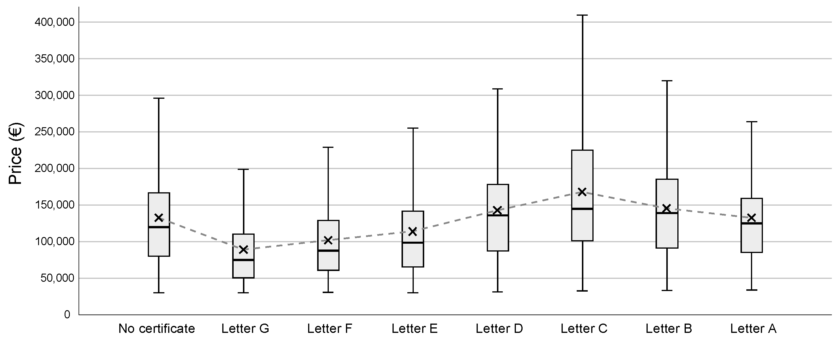
| Letter G | 3040 | 89,216.5 | |||
| Letter F | 864 | 102,037.9 | 102,037.9 | ||
| Letter E | 3083 | 113,680.5 | |||
| NT (no label) | 43,745 | 132,699.2 | |||
| Letter A | 807 | 133,694.0 | |||
| Letter D | 587 | 142,756.2 | |||
| Letter B | 325 | 145,554.3 | |||
| Letter C | 488 | 168,049.7 | |||
| Sig. | 0.055 | 0.123 | 0.053 | 1.000 | |
| Variable | Estimates | ||||||||
|---|---|---|---|---|---|---|---|---|---|
| 1 | 2 | 3 | 4 | 5 | 6 | 7 | 8 | 9 | |
| ABCDEFG/Ref.NT | A/Ref.NT | A/B/C/D/E/F/G/Ref.NT | A/B/C/Ref.D/E/F/G | ABC/Ref.D/EFG | AB/C/Ref.D/E/F/G | A/B/C/D/E/F/Ref.G | ABC/D/E/F/Ref.G | AB/C/D/E/F/Ref.G | |
| Intercept | 10.099 *** (0.011) | 10.082 *** (0.011) | 10.102 *** (0.011) | 10.225 *** (0.029) | 10.216 *** (0.029) | 10.228 *** (0.029) | 10.137 *** (0.026) | 10.131 *** (0.026) | 10.141 *** (0.026) |
| Dwelling characteristics (A) | |||||||||
| A_age | −0.0005 *** (0.0001) | 0.0001 (0.0002) | −0.0005 *** (0.0001) | −0.0029 *** (0.0003) | −0.0029 *** (0.0003) | −0.0029 *** (0.0003) | −0.0029 *** (0.0003) | −0.0029 *** (0.0003) | −0.0029 *** (0.0003) |
| A_area_m2 | 0.0058 *** (0.0001) | 0.0058 *** (0.0001) | 0.0058 *** (0.0001) | 0.0058 *** (0.0002) | 0.0058 *** (0.0002) | 0.0058 *** (0.0002) | 0.0058 *** (0.0002) | 0.0058 *** (0.0002) | 0.0058 *** (0.0002) |
| A_bedrooms | −0.002 (0.002) | 0.004 (0.003) | −0.002 (0.002) | −0.021 *** (0.006) | −0.021 *** (0.006) | −0.021 *** (0.006) | −0.021 *** (0.006) | −0.021 *** (0.006) | −0.021 *** (0.006) |
| A_bathrooms | 0.217 *** (0.003) | 0.214 *** (0.004) | 0.216 *** (0.003) | 0.224 *** (0.008) | 0.225 *** (0.008) | 0.225 *** (0.008) | 0.224 *** (0.008) | 0.225 *** (0.008) | 0.225 *** (0.008) |
| A_wardrobe | 0.013 *** (0.003) | 0.015 *** (0.003) | 0.012 *** (0.003) | 0.002 (0.009) | 0.003 (0.009) | 0.002 (0.009) | 0.002 (0.009) | 0.002 (0.009) | 0.002 (0.009) |
| A_air_cond | 0.077 *** (0.003) | 0.074 *** (0.003) | 0.076 *** (0.003) | 0.084 *** (0.008) | 0.086 *** (0.008) | 0.084 *** (0.008) | 0.084 *** (0.008) | 0.086 *** (0.008) | 0.084 *** (0.008) |
| A_terrace | 0.009 ** (0.003) | 0.006 * (0.003) | 0.008 ** (0.003) | 0.028 *** (0.008) | 0.029 *** (0.008) | 0.028 *** (0.008) | 0.028 *** (0.008) | 0.029 *** (0.008) | 0.028 *** (0.008) |
| A_floor | 0.004 *** (0.001) | 0.004 *** (0.001) | 0.004 *** (0.001) | 0.0002 (0.002) | 0.0002 (0.002) | 0.0001 (0.002) | 0.0002 (0.002) | 0.0002 (0.002) | 0.0001 (0.002) |
| A_new_construction | 0.224 *** (0.013) | 0.224 *** (0.014) | 0.222 *** (0.013) | 0.208 *** (0.038) | 0.191 *** (0.038) | 0.189 *** (0.038) | 0.208 *** (0.038) | 0.190 *** (0.038) | 0.189 *** (0.038) |
| A_state_to_reform | −0.151 *** (0.006) | −0.168 *** (0.007) | −0.152 *** (0.006) | −0.095 *** (0.013) | −0.094 *** (0.013) | −0.095 *** (0.013) | −0.095 *** (0.013) | −0.095 *** (0.013) | −0.095 *** (0.013) |
| A_good_condition (Ref.) | |||||||||
| A_flat (Ref.) | |||||||||
| A_studio_flat | −0.223 *** (0.013) | −0.214 *** (0.014) | −0.223 *** (0.013) | −0.236 *** (0.033) | −0.235 *** (0.033) | −0.233 *** (0.033) | −0.236 *** (0.033) | −0.236 *** (0.033) | −0.233 *** (0.033) |
| A_penthouse | 0.108 *** (0.006) | 0.112 *** (0.006) | 0.108 *** (0.006) | 0.095 *** (0.016) | 0.091 *** (0.016) | 0.094 *** (0.016) | 0.095 *** (0.016) | 0.091 *** (0.016) | 0.094 *** (0.016) |
| A_duplex | 0.044 *** (0.008) | 0.049 *** (0.008) | 0.044 *** (0.008) | 0.013 (0.021) | 0.010 (0.021) | 0.012 (0.021) | 0.013 (0.021) | 0.010 (0.021) | 0.012 (0.021) |
| ABCDEFG | −0.032 *** (0.004) | ||||||||
| ABC | −0.025 (0.015) | 0.062 *** (0.011) | |||||||
| AB | −0.046 ** (0.016) | 0.041 ** (0.013) | |||||||
| A | −0.003 (0.010) | −0.002 (0.010) | −0.026 (0.017) | 0.061 *** (0.014) | |||||
| B | −0.080 *** (0.016) | −0.091 *** (0.021) | −0.003 (0.019) | ||||||
| C | 0.049 *** (0.013) | 0.014 (0.019) | 0.015 (0.019) | 0.101 *** (0.016) | 0.102 *** (0.016) | ||||
| D | 0.033 ** (0.012) | Ref. | Ref. | Ref. | 0.087 *** (0.014) | 0.088 *** (0.014) | 0.087 *** (0.014) | ||
| E | −0.043 *** (0.006) | −0.081 *** (0.014) | −0.081 *** (0.014) | 0.006 (0.008) | 0.006 (0.008) | 0.006 (0.008) | |||
| F | −0.038 *** (0.010) | −0.080 *** (0.016) | −0.079 *** (0.016) | 0.008 (0.012) | 0.007 (0.012) | 0.008 (0.012) | |||
| G | −0.053 *** (0.006) | −0.087 *** (0.014) | −0.087 *** (0.014) | Ref. | Ref. | Ref. | |||
| EFG | −0.083 *** (0.013) | ||||||||
| NT (no label) | Ref. | Ref. | Ref. | ||||||
| Building characteristics (B) | |||||||||
| B_elevator | 0.185 *** (0.003) | 0.179 *** (0.004) | 0.183 *** (0.003) | 0.195 *** (0.008) | 0.196 *** (0.008) | 0.195 *** (0.008) | 0.195 *** (0.008) | 0.195 *** (0.008) | 0.195 *** (0.008) |
| B_parking | 0.111 *** (0.003) | 0.111 *** (0.003) | 0.110 *** (0.003) | 0.102 *** (0.009) | 0.102 *** (0.009) | 0.101 *** (0.009) | 0.102 *** (0.009) | 0.102 *** (0.009) | 0.101 *** (0.009) |
| B_storeroom | 0.048 *** (0.003) | 0.048 *** (0.003) | 0.047 *** (0.003) | 0.049 *** (0.009) | 0.048 *** (0.010) | 0.049 *** (0.010) | 0.049 *** (0.009) | 0.048 *** (0.010) | 0.049 *** (0.010) |
| B_pool | 0.092 *** (0.004) | 0.093 *** (0.004) | 0.092 *** (0.004) | 0.094 *** (0.011) | 0.093 *** (0.011) | 0.093 *** (0.011) | 0.094 *** (0.011) | 0.092 *** (0.011) | 0.093 *** (0.011) |
| B_garden | 0.034 *** (0.004) | 0.037 *** (0.004) | 0.034 *** (0.004) | −0.002 (0.011) | −0.002 (0.011) | −0.002 (0.011) | −0.002 (0.011) | −0.002 (0.011) | −0.002 (0.011) |
| Location characteristics (C) | |||||||||
| C_Alicante (Ref.) | |||||||||
| C_Marina_Alta | 0.004 (0.005) | 0.031 *** (0.006) | 0.006 (0.005) | −0.097 *** (0.013) | −0.099 *** (0.013) | −0.097 *** (0.013) | −0.097 *** (0.013) | −0.099 *** (0.013) | −0.097 *** (0.013) |
| C_Marina_Baja | 0.098 *** (0.005) | 0.115 *** (0.006) | 0.098 *** (0.005) | 0.018 (0.014) | 0.014 (0.014) | 0.016 (0.014) | 0.018 (0.014) | 0.014 (0.014) | 0.016 (0.014) |
| C_Bajo_Vinalopo | 0.016 ** (0.005) | 0.020 *** (0.005) | 0.015 ** (0.005) | −0.004 (0.013) | −0.005 (0.013) | −0.003 (0.013) | −0.004 (0.013) | −0.004 (0.013) | −0.003 (0.013) |
| C_Bajo_Segura | −0.207 *** (0.005) | −0.211 *** (0.006) | −0.206 *** (0.005) | −0.194 *** (0.012) | −0.194 *** (0.012) | −0.194 *** (0.012) | −0.194 *** (0.012) | −0.194 *** (0.012) | −0.194 *** (0.012) |
| C_Condado | −0.164 *** (0.021) | −0.164 *** (0.023) | −0.164 *** (0.021) | −0.186 *** (0.056) | −0.192 *** (0.056) | −0.188 *** (0.056) | −0.186 *** (0.056) | −0.192 *** (0.056) | −0.188 *** (0.056) |
| C_Alcoy | −0.210 *** (0.010) | −0.214 *** (0.011) | −0.211 *** (0.010) | −0.193 *** (0.022) | −0.192 *** (0.022) | −0.191 *** (0.022) | −0.193 *** (0.022) | −0.192 *** (0.022) | −0.191 *** (0.022) |
| C_Alto_Vinalopo | −0.135 *** (0.016) | −0.116 *** (0.019) | −0.134 *** (0.016) | −0.155 *** (0.028) | −0.156 *** (0.028) | −0.156 *** (0.028) | −0.155 *** (0.028) | −0.156 *** (0.028) | −0.156 *** (0.028) |
| C_Medio_Vinalopo | −0.185 *** (0.009) | −0.186 *** (0.010) | −0.186 *** (0.009) | −0.196 *** (0.020) | −0.196 *** (0.020) | −0.196 *** (0.020) | −0.196 *** (0.020) | −0.196 *** (0.020) | −0.196 *** (0.020) |
| C_dist_pharmacy | −0.017 *** (0.003) | −0.021 *** (0.003) | −0.017 *** (0.003) | −0.005 (0.007) | −0.004 (0.007) | −0.005 (0.007) | −0.005 (0.007) | −0.004 (0.007) | −0.005 (0.007) |
| C_dist_health | 0.008 *** (0.001) | 0.007 *** (0.001) | 0.008 *** (0.001) | 0.017 *** (0.003) | 0.016 *** (0.003) | 0.017 *** (0.003) | 0.017 *** (0.003) | 0.016 *** (0.003) | 0.017 *** (0.003) |
| C_dist_hospital | 0.002 *** (0.000) | 0.002 *** (0.000) | 0.002 *** (0.000) | 0.003 *** (0.001) | 0.003 *** (0.001) | 0.003 *** (0.001) | 0.003 *** (0.001) | 0.003 *** (0.001) | 0.003 *** (0.001) |
| C_dist_educ1 | 0.027 *** (0.002) | 0.026 *** (0.003) | 0.026 *** (0.002) | 0.021 *** (0.006) | 0.021 *** (0.006) | 0.021 *** (0.006) | 0.021 *** (0.006) | 0.021 *** (0.006) | 0.021 *** (0.006) |
| C_dist_educ2 | −0.021 *** (0.001) | −0.022 *** (0.001) | −0.021 *** (0.001) | −0.012 *** (0.003) | −0.012 *** (0.003) | −0.012 *** (0.003) | −0.012 *** (0.003) | −0.012 *** (0.003) | −0.012 *** (0.003) |
| C_coastalregion | 0.146 *** (0.004) | 0.140 *** (0.004) | 0.145 *** (0.004) | 0.166 *** (0.009) | 0.165 *** (0.009) | 0.165 *** (0.009) | 0.166 *** (0.009) | 0.165 *** (0.009) | 0.165 *** (0.009) |
| C_FAR | −0.026 *** (0.002) | −0.027 *** (0.002) | −0.027 *** (0.002) | −0.018 *** (0.005) | −0.017 ** (0.005) | −0.018 *** (0.005) | −0.018 *** (0.005) | −0.017 *** (0.005) | −0.018 *** (0.005) |
| Neighborhood characteristics (D) | |||||||||
| D_dependency | 0.221 *** (0.008) | 0.237 *** (0.009) | 0.220 *** (0.008) | 0.157 *** (0.021) | 0.161 *** (0.021) | 0.159 *** (0.021) | 0.157 *** (0.021) | 0.161 *** (0.021) | 0.159 *** (0.021) |
| D_elderly | 0.009 *** (0.001) | 0.008 *** (0.001) | 0.009 *** (0.001) | 0.011 *** (0.002) | 0.010 *** (0.002) | 0.011 *** (0.002) | 0.011 *** (0.002) | 0.011 *** (0.002) | 0.011 *** (0.002) |
| D_foreigners | 0.001 *** (0.000) | 0.001 *** (0.000) | 0.001 *** (0.000) | 0.001 *** (0.000) | 0.001 *** (0.000) | 0.001 *** (0.000) | 0.001 *** (0.000) | 0.001 *** (0.000) | 0.001 *** (0.000) |
| D_no_studies | −0.008 *** (0.000) | −0.008 *** (0.000) | −0.008 *** (0.000) | −0.005 *** (0.001) | −0.005 *** (0.001) | −0.005 *** (0.001) | −0.005 *** (0.001) | −0.005 *** (0.001) | −0.005 *** (0.001) |
| D_university | 0.009 *** (0.000) | 0.009 *** (0.000) | 0.009 *** (0.000) | 0.008 *** (0.000) | 0.009 *** (0.000) | 0.009 *** (0.000) | 0.008 *** (0.000) | 0.009 *** (0.000) | 0.009 *** (0.000) |
| Market characteristics (E) | |||||||||
| E_professional | −0.028 *** (0.003) | −0.028 *** (0.004) | −0.025 *** (0.003) | −0.006 (0.010) | −0.002 (0.009) | −0.010 (0.010) | −0.006 (0.010) | −0.002 (0.009) | −0.010 (0.010) |
| E_private(Ref.) | |||||||||
| E_bank | −0.003 (0.010) | −0.103 *** (0.029) | 0.005 (0.010) | −0.006 (0.015) | −0.0004 (0.014) | −0.010 (0.015) | −0.006 (0.015) | −0.002 (0.015) | −0.010 (0.015) |
| E_secondary_dw | 0.003 *** (0.000) | 0.003 *** (0.000) | 0,003 *** (0.000) | 0.002 *** (0.000) | 0.002 *** (0.000) | 0.002 *** (0.000) | 0.002 *** (0.000) | 0.002 *** (0.000) | 0.002 *** (0.000) |
| E_rented_dw | 0.003 *** (0.000) | 0.002 *** (0.000) | 0.003 *** (0.000) | 0.003 *** (0.000) | 0.003 *** (0.000) | 0.003 *** (0.000) | 0.003 *** (0.000) | 0.003 *** (0.000) | 0.003 *** (0.000) |
| N | 52,939 | 44,552 | 52,939 | 9194 | 9194 | 9194 | 9194 | 9194 | 9194 |
| R2 | 0.708 | 0.702 | 0.708 | 0.716 | 0.716 | 0.716 | 0.716 | 0.716 | 0.716 |
| adj. R2 | 0.708 | 0.702 | 0.708 | 0.715 | 0.714 | 0.715 | 0.715 | 0.714 | 0.715 |
| Std. Error | 0.29 | 0.29 | 0.29 | 0.30 | 0.30 | 0.30 | 0.30 | 0.30 | 0.30 |
| F (sig.) | 2979 *** | 2442 *** | 2621 *** | 481 *** | 523 *** | 490 *** | 481 *** | 500 *** | 490 *** |
| Durbin-Watson | 1.89 | 1.91 | 1.89 | 1.79 | 1.79 | 1.79 | 1.79 | 1.79 | 1.79 |
| Study Data | Economic Price Premium in % According to the Reference-Ref.-(Certificate Letter or Group of Letters) | Compared with | |||||||||||||
|---|---|---|---|---|---|---|---|---|---|---|---|---|---|---|---|
| Paper | Country | Estim. | ABC | AB | A | B | C | D | E | F | G | FG | EFG | NT | |
| [21] | Netherlands | 2 (Table 3) | 10.2 * | 5.6 * | 2.2 * | Ref. | −0.5 | −2.5 * | −5.1 * | Estim. 4 | |||||
| [69] | Portugal | 2 (Table 5) | 5.94 * | Ref. | −4.03 * | Estim. 5 | |||||||||
| [25] | United Kingdom | 4 (Table 4) | 1.6 * | 0.8 * | Ref. | −1.4 * | −2.9 * | −7.2 * | Estim. 6 | ||||||
| [26] | United Kingdom | 7 (Table 2) | 3.6 | 3.9 | Ref. | −8.2 | −10.5 | −15.0 | Estim. 6 | ||||||
| [18] | Denmark | 3 (Table 1) | 6.6 * | 0.2 | Ref. | −1.5 * | −3.5 * | −9.3 * | Estim. 6 | ||||||
| 4 (Table 1) | 6.2 * | 5.1 * | Ref. | −5.4 * | −12.9 * | −24.3 * | Estim. 6 | ||||||||
| [23] | Ireland | 1 (Table 4) | 9.3 * | 5.2 * | 1.7 * | Ref. | −0.4 | −10.6 * | - | ||||||
| [19] | France | Occitainie | 14.0 * | 3.0 * | Ref. | −4.0 * | −6.0 * | - | |||||||
| [20] | France | Provence | 6.0 * | 2.0 * | Ref. | −3.0 * | −10.0 * | - | |||||||
| [70] | Germany | 8 (Table II) | - | 0.76 * | 0.65 * | 0.75 * | 0.87 * | 0.30 * | Ref. | - | |||||
| [24] | Italy | 1 (Table 2) | 21.9 * | 20.2 * | 17.4 * | 17.1 * | 9.5 * | 2.3 | Ref. | Estim. 7 | |||||
| [31] | Spain | 5BCN | 10.0 * | - | 6.0 * | 7.0 * | 2.0 | 1.0 * | Ref. | Estim. 7 | |||||
| 5VIC | 29.0 * | - | 18.0 | 16.0 * | 4.0 * | −2.0 | Ref. | Estim. 7 | |||||||
| 5ALC | 8.0 * | - | −23.0 * | 2.0 | −5.0 * | −5.0 * | Ref. | Estim. 7 | |||||||
| [16] | Spain | 3B (Table 4) | 9.62 * | - | −3.0 | 3.87 * | 2.0 | 1.0 | Ref. | Estim. 7 | |||||
| [17] | Spain | 3 (Table 3) | −6.3 * | 1.9 | 1.1 * | 1.8 * | Ref. | Estim. 8 | |||||||
| [27] | United Kingdom | 5 (Table 5) | 11.6 * | 10.4 * | 9.3 * | 8.0 * | 5.6 * | Ref. | Estim. 9 | ||||||
| [22] | Netherlands | 4 (Table 2) | 5.6 * | 1.1 * | −0.2 | −0.8 * | −1.4 * | −1.6 * | −0.8 | Ref. | Estim. 3 | ||||
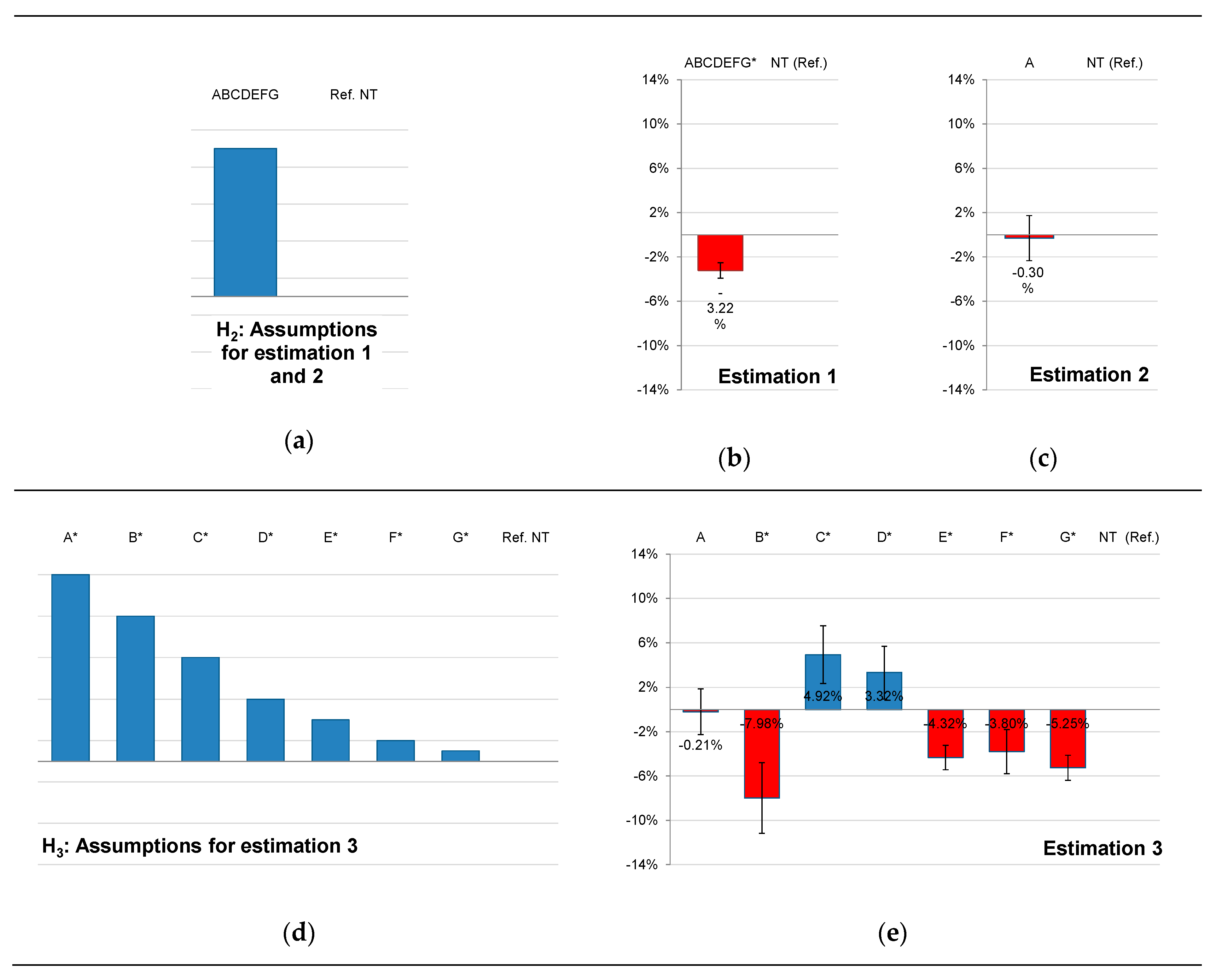
| This research | Spain | 3 | −0.2 | −8.0 * | 4.9 * | 3.3 * | −4.3 * | −3.8 * | −5.3 * | Ref. | [22] | ||||
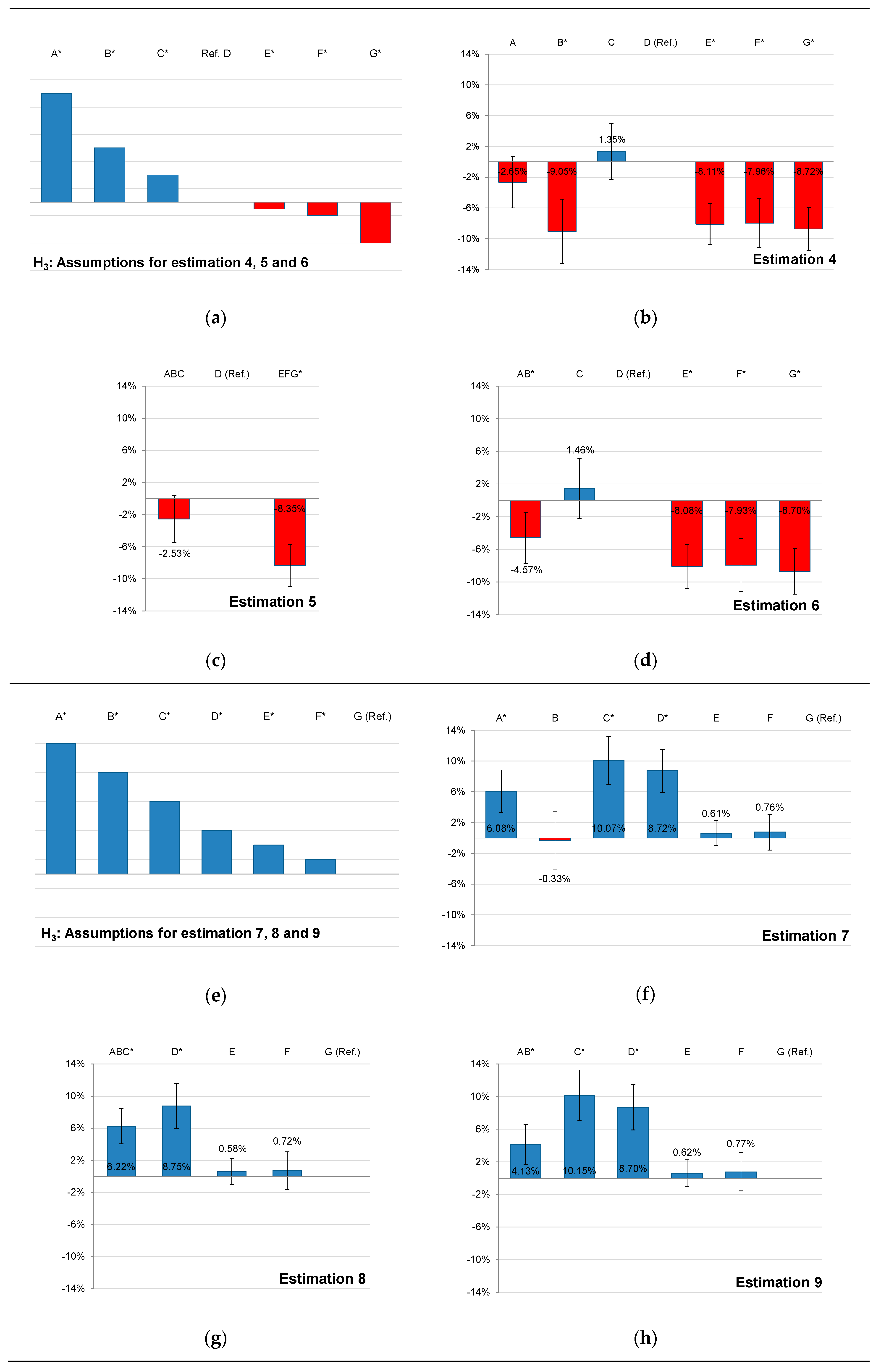
| 4 | −2.7 | −9.1 * | 1.4 | Ref. | −8.1 * | −8.0 * | −8.7 * | [21] | |||||||
| 5 | −2.5 | Ref. | −8.4 * | [69] | |||||||||||
| 6 | −4.6 * | 1.5 | Ref. | −8.1 * | −7.9 * | −8.7 * | [18,25,26] | ||||||||
| 7 | 6.1 * | −0.3 | 10.1 * | 8.7 * | 0.6 | 0.8 | Ref. | [16,24,31] | |||||||
| 8 | 6.2 * | 8.8 * | 0.6 | 0.7 | Ref. | [17] | |||||||||
| 9 | 4.1 * | 10.2 * | 8.7 * | 0.6 | 0.8 | Ref. | [27] | ||||||||
© 2020 by the authors. Licensee MDPI, Basel, Switzerland. This article is an open access article distributed under the terms and conditions of the Creative Commons Attribution (CC BY) license (http://creativecommons.org/licenses/by/4.0/).
Share and Cite
Cespedes-Lopez, M.-F.; Mora-Garcia, R.-T.; Perez-Sanchez, V.R.; Marti-Ciriquian, P. The Influence of Energy Certification on Housing Sales Prices in the Province of Alicante (Spain). Appl. Sci. 2020, 10, 7129. https://0-doi-org.brum.beds.ac.uk/10.3390/app10207129
Cespedes-Lopez M-F, Mora-Garcia R-T, Perez-Sanchez VR, Marti-Ciriquian P. The Influence of Energy Certification on Housing Sales Prices in the Province of Alicante (Spain). Applied Sciences. 2020; 10(20):7129. https://0-doi-org.brum.beds.ac.uk/10.3390/app10207129
Chicago/Turabian StyleCespedes-Lopez, Maria-Francisca, Raul-Tomas Mora-Garcia, V. Raul Perez-Sanchez, and Pablo Marti-Ciriquian. 2020. "The Influence of Energy Certification on Housing Sales Prices in the Province of Alicante (Spain)" Applied Sciences 10, no. 20: 7129. https://0-doi-org.brum.beds.ac.uk/10.3390/app10207129