Convection Heat Transfer in 3D Wavy Direct Absorber Solar Collector Based on Two-Phase Nanofluid Approach

 ,
,
Abstract
:
1. Introduction
2. Mathematical Formulation
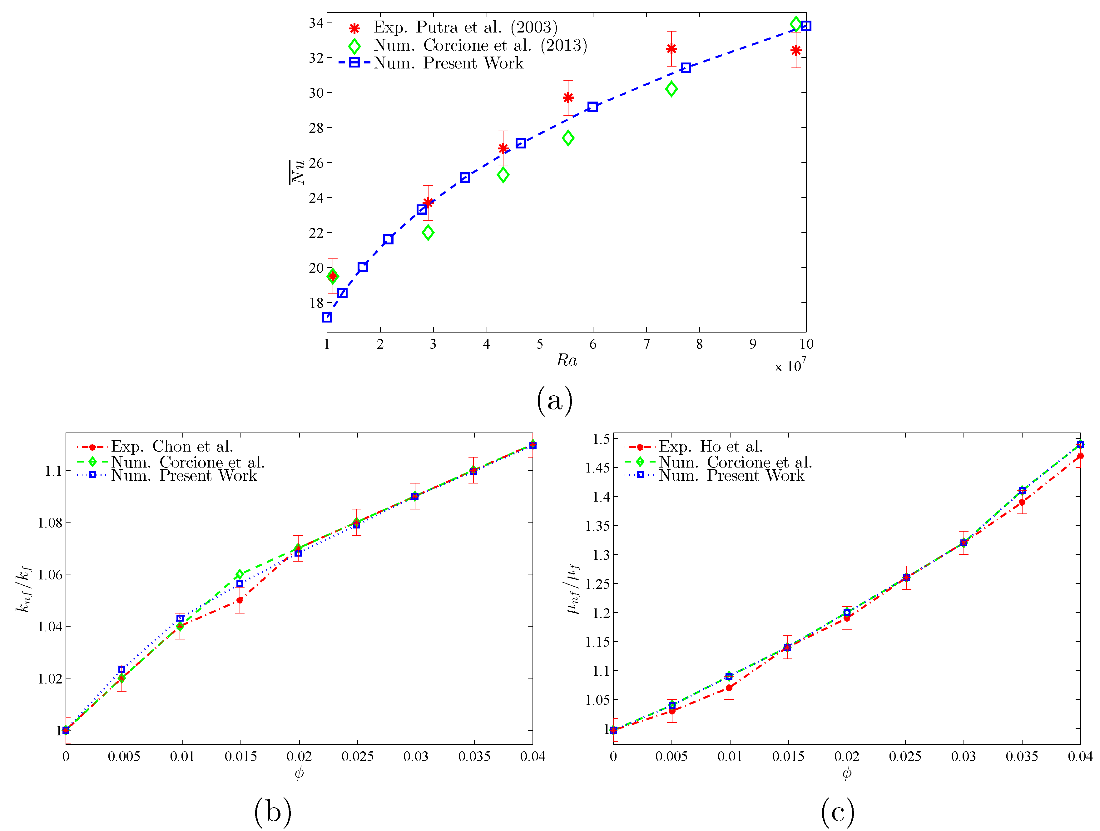
3. Numerical Method and Validation
4. Results and Discussion
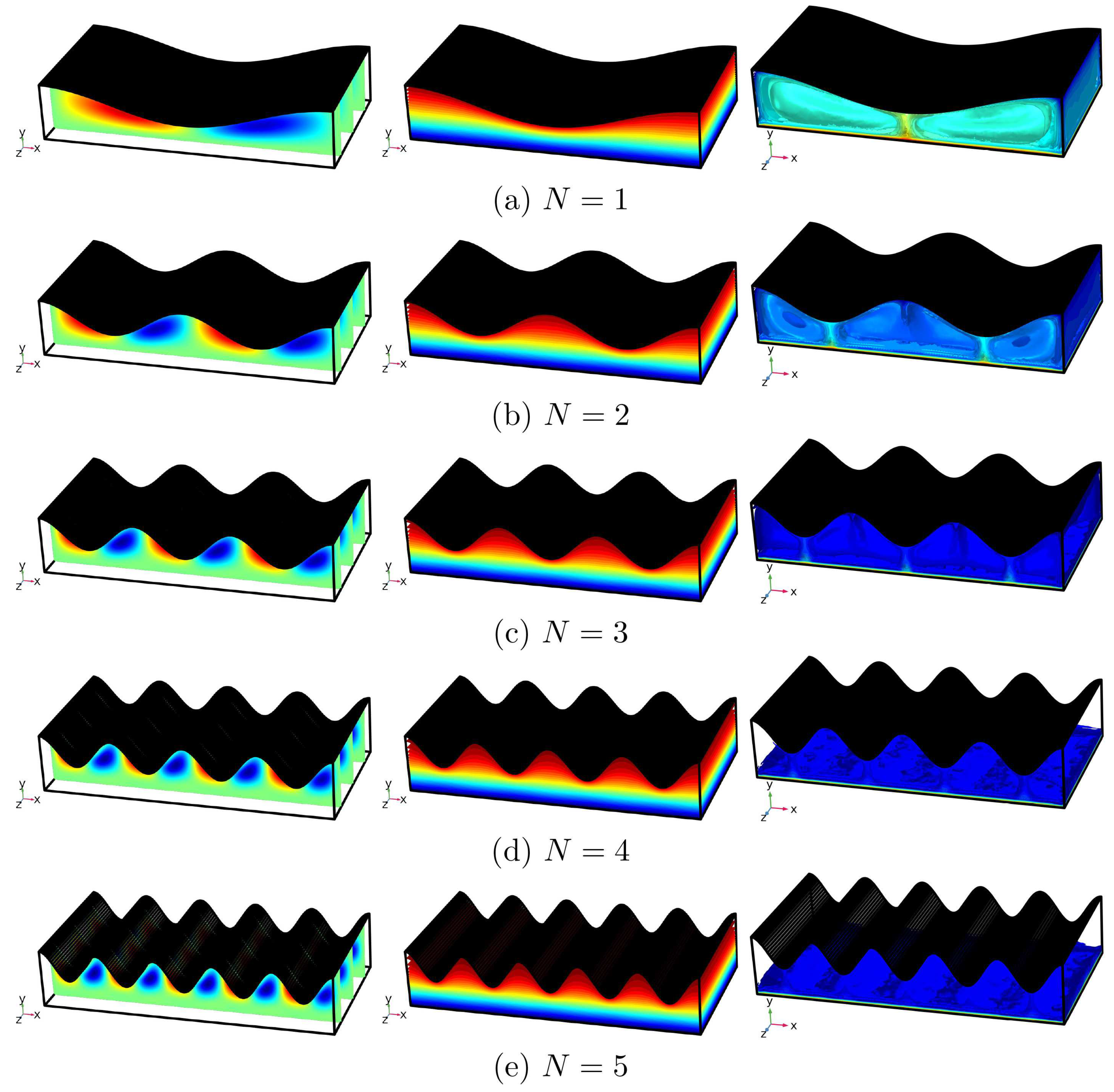
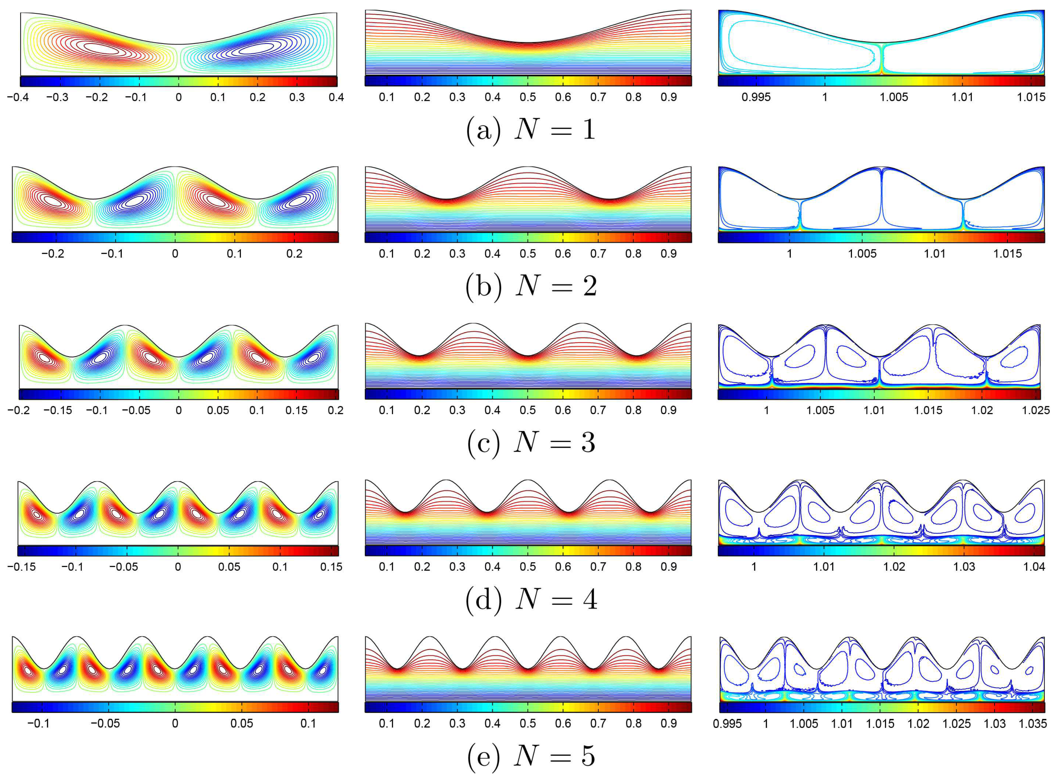
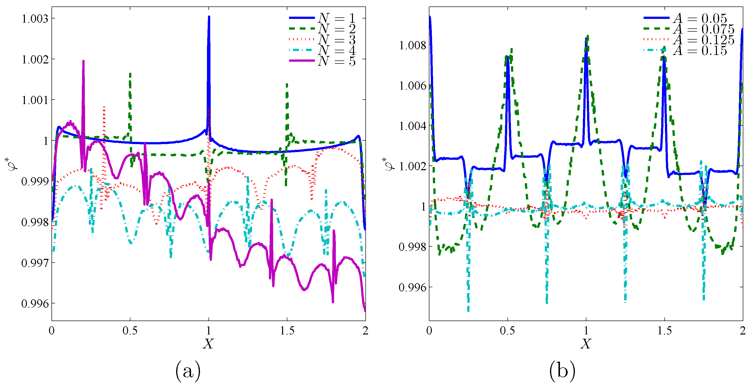
4.1. Outcomes of Number of Oscillations (N)
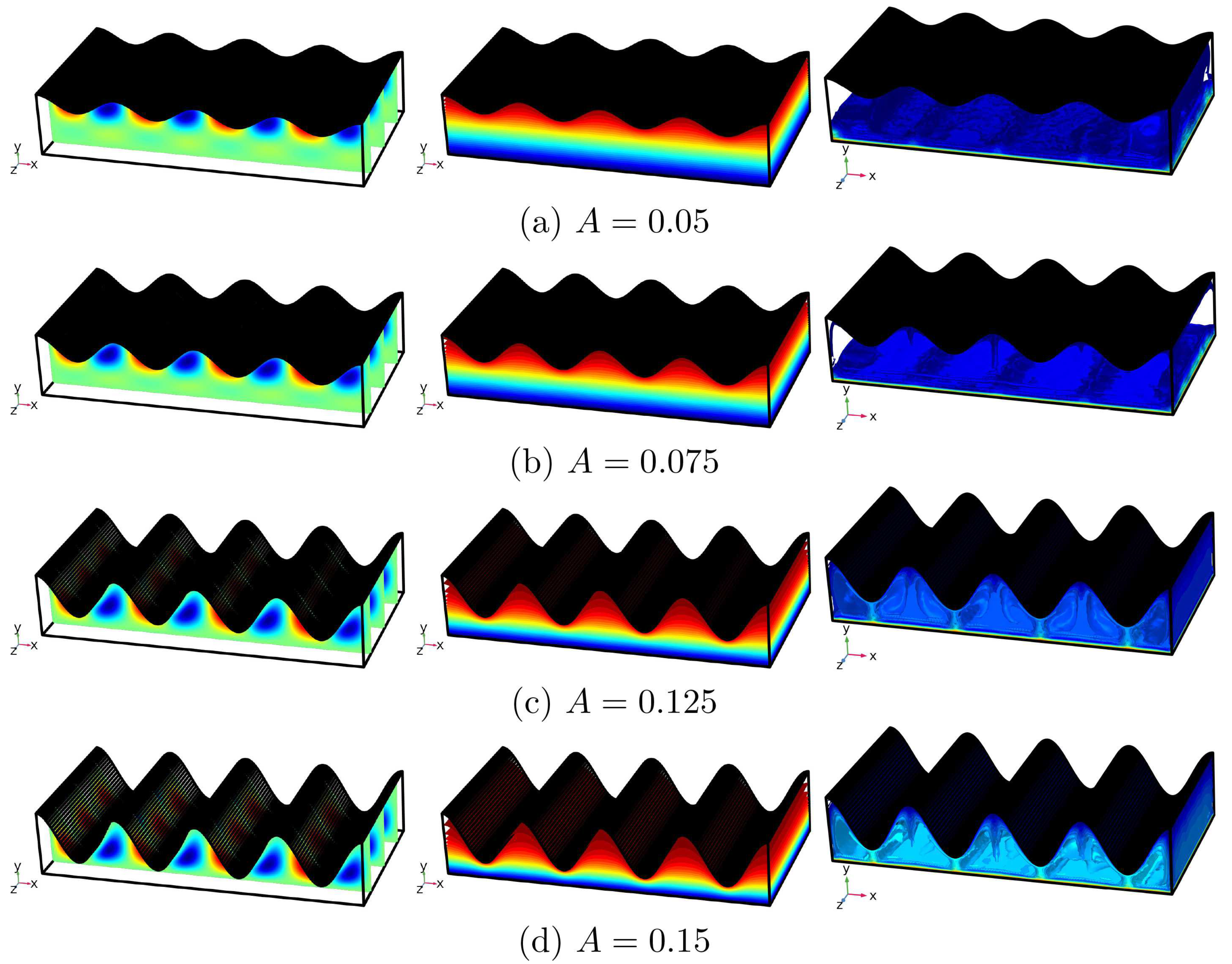
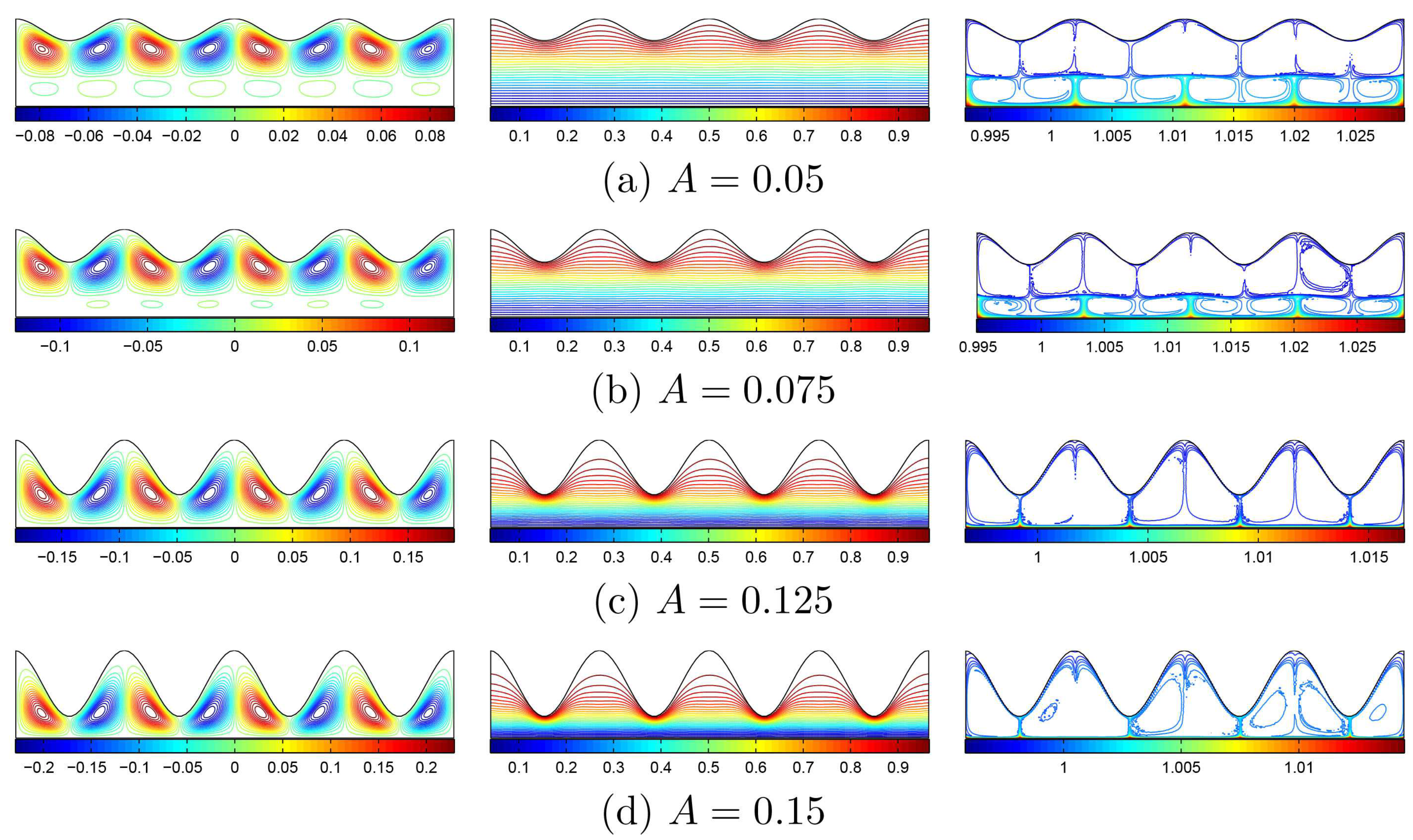
4.2. Outcomes of Wave Amplitude (A)
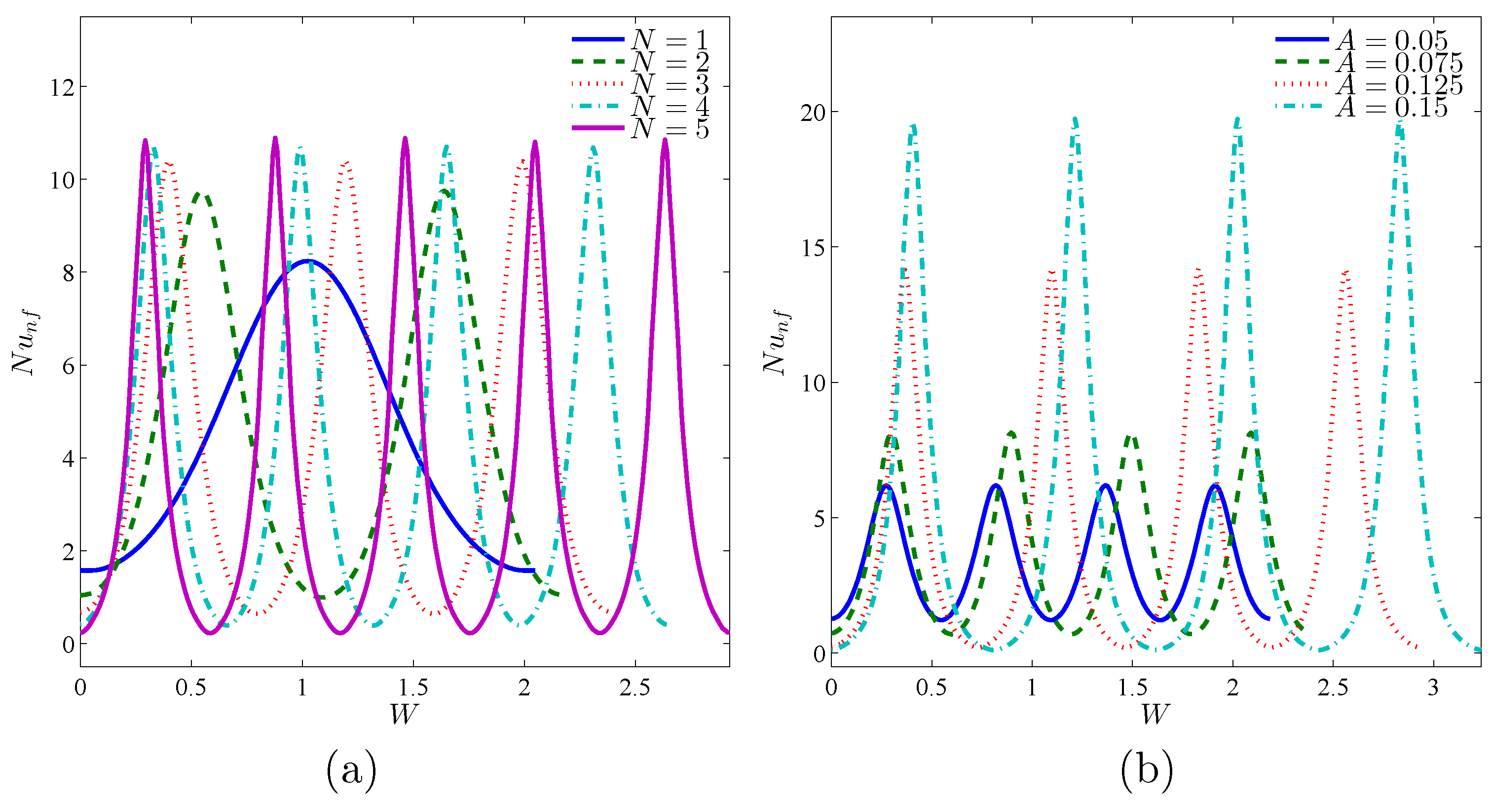
4.3. Variation of the Nusselt Number
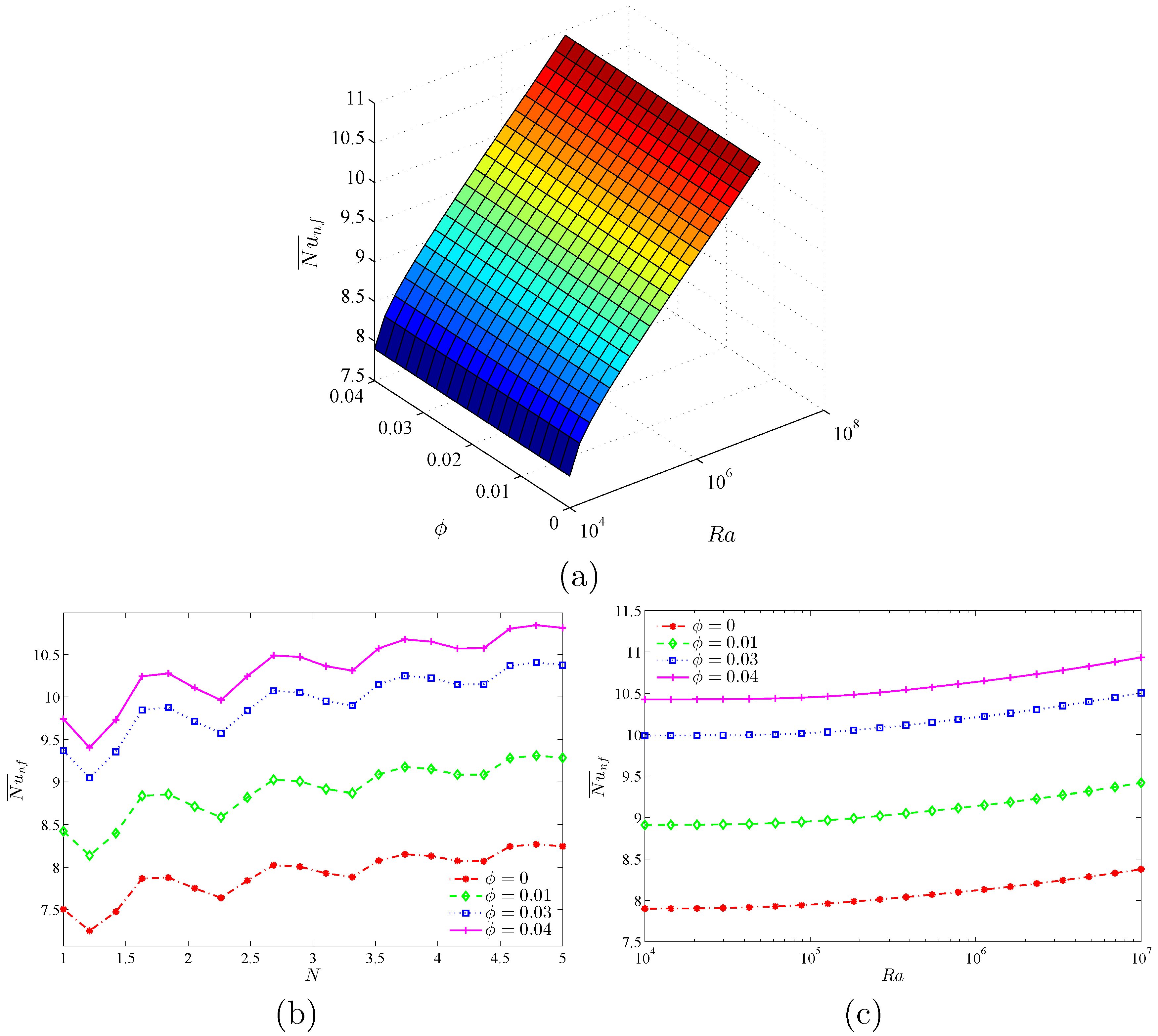
4.4. Outcomes of Rayleigh Number ()
4.5. Outcomes of Solid Volume Fraction ()
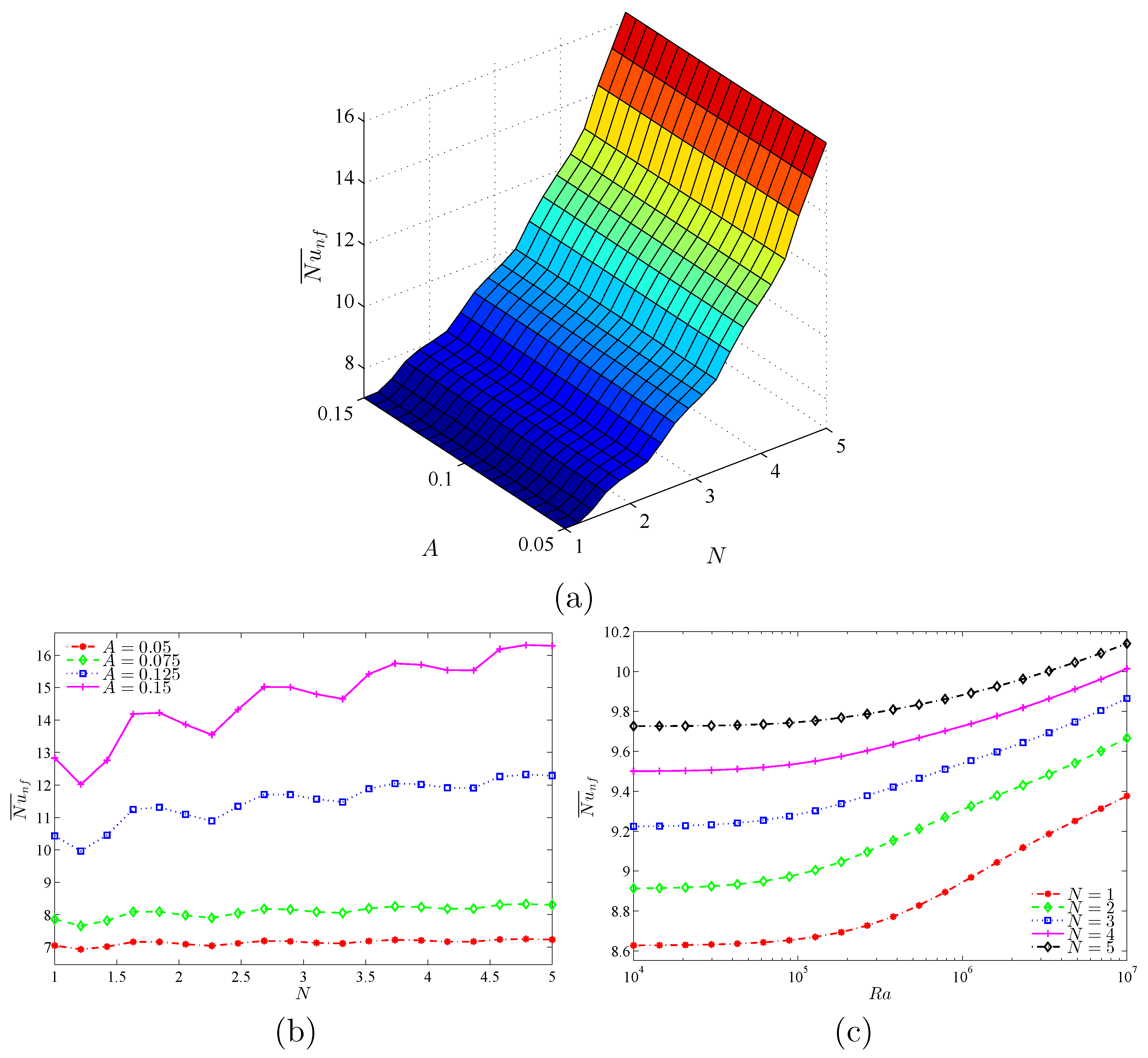
4.6. Variation of the Nusselt Number
5. Conclusions
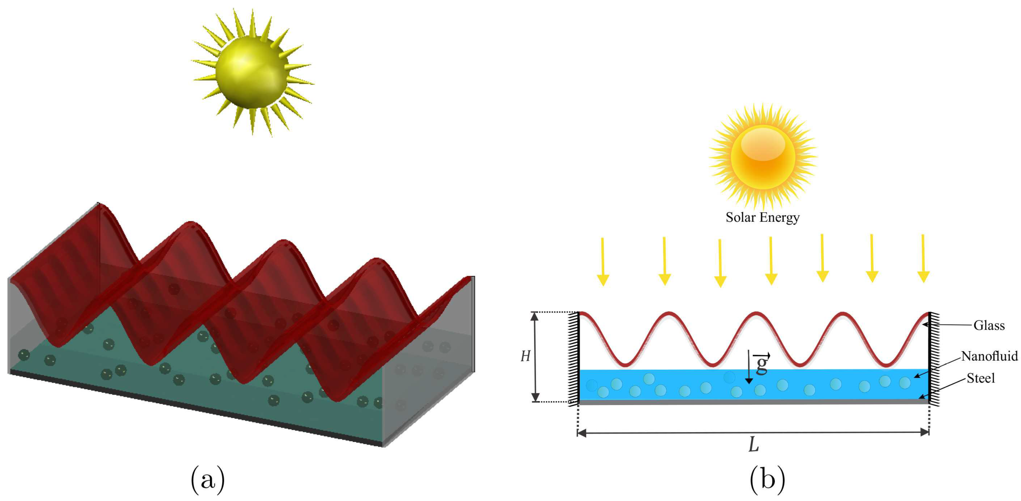
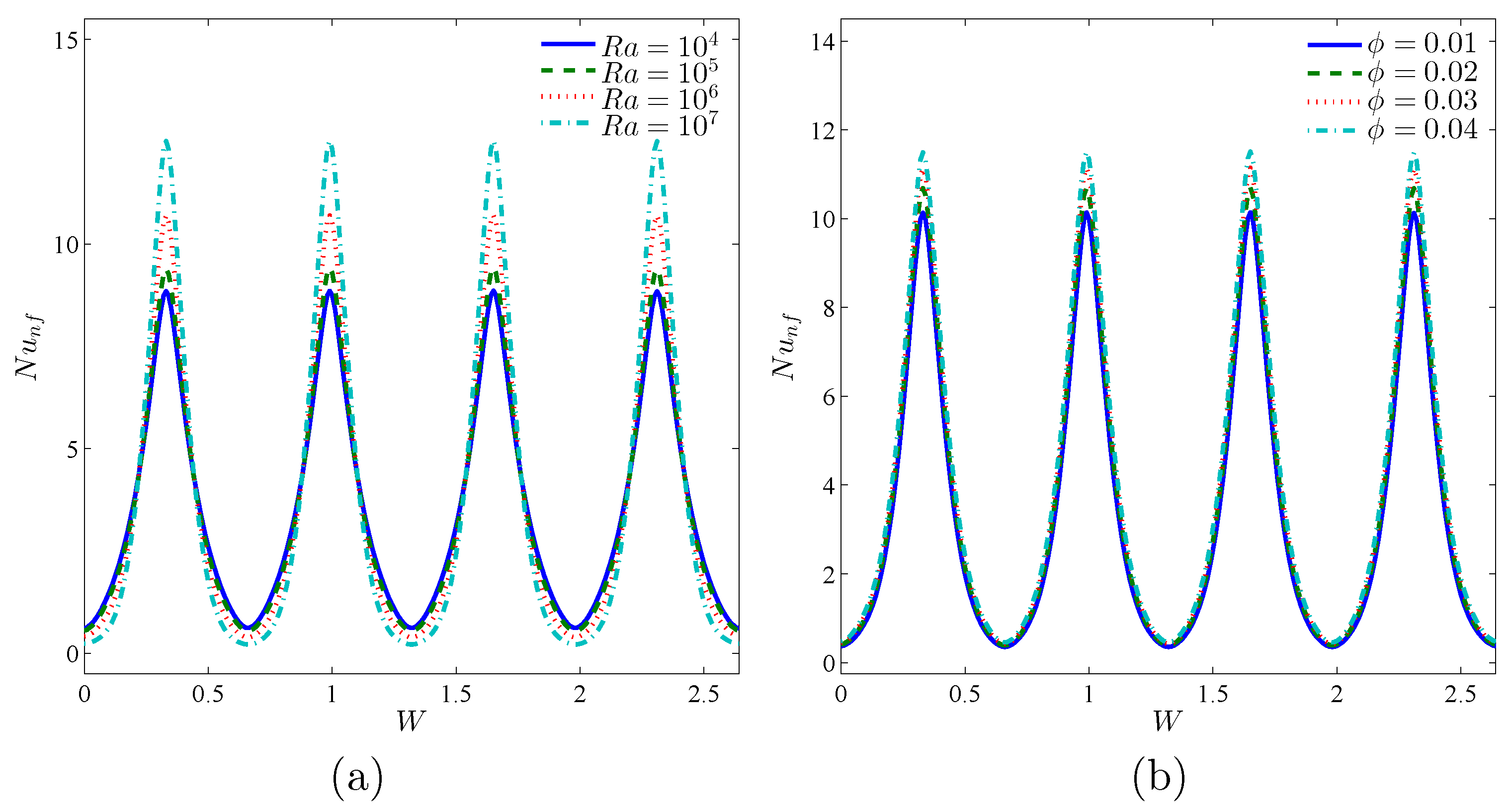
- Increasing the number of oscillations leads to a higher temperature gradient region which is extended to the five concave portions of the top wall due to the extra energy of the upper wall.
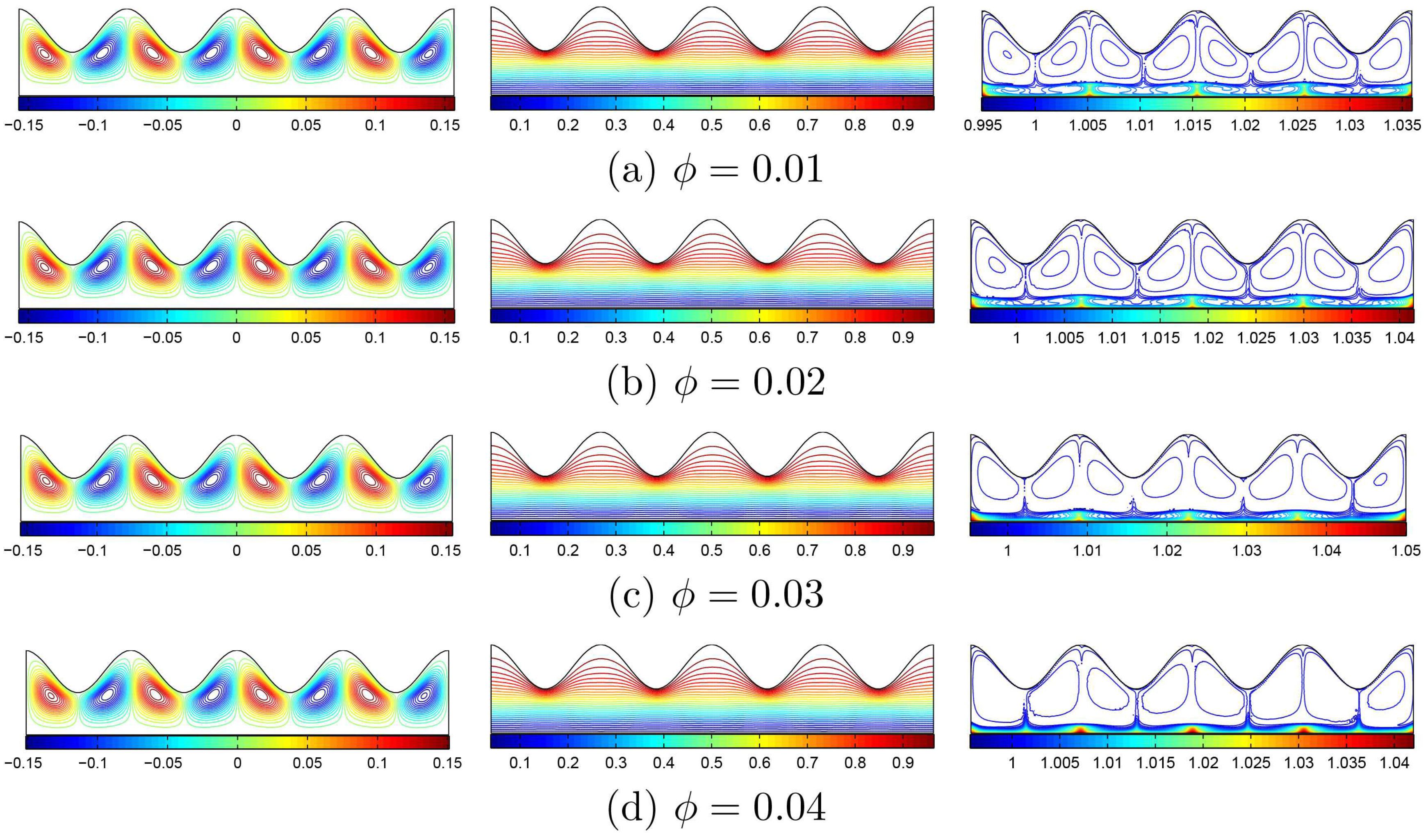
- It is found that an augmentation of the wave amplitude enhances the thermophoresis and Brownian influences, which clearly force the nanoparticles concentration to display a completely nonuniform trend in the region.
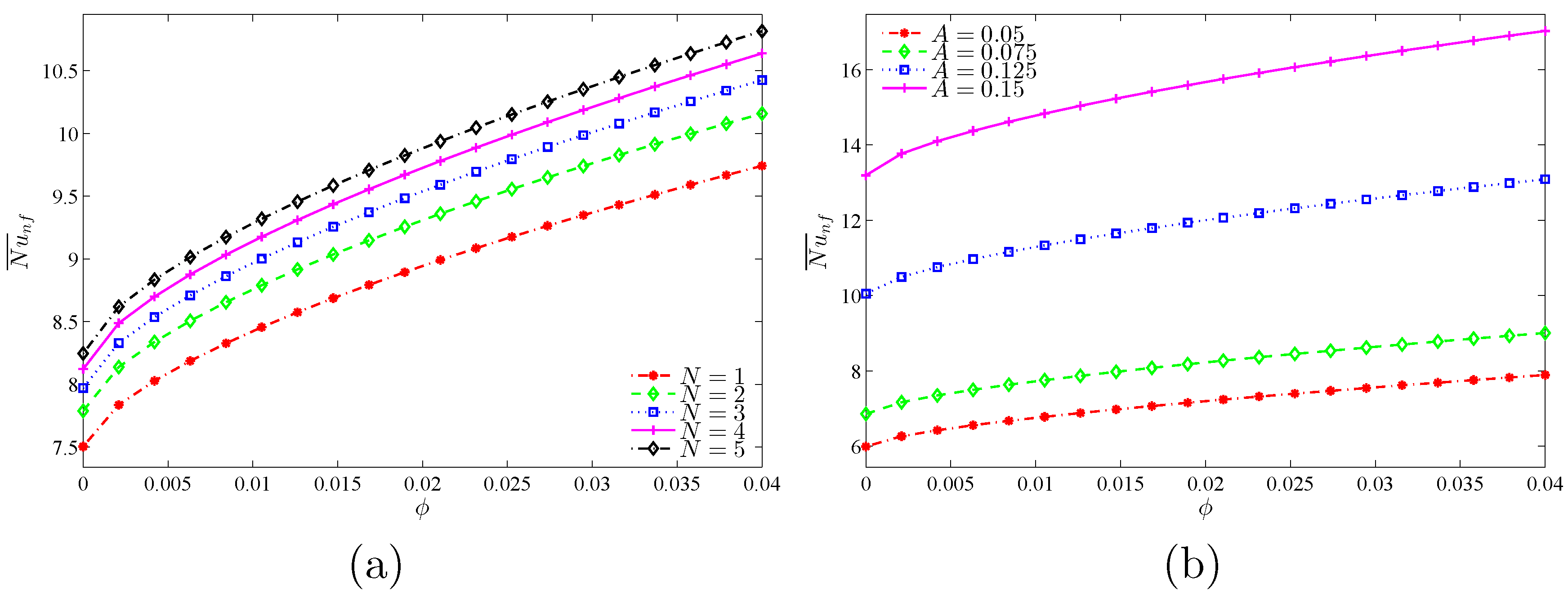
- An augmentation in the local heat transfer is observed for both cases when increasing the number of waves as well as the wave amplitudes. However, this augmentation in the heat transfer is noticed to be higher by considering the role of the wave amplitude.
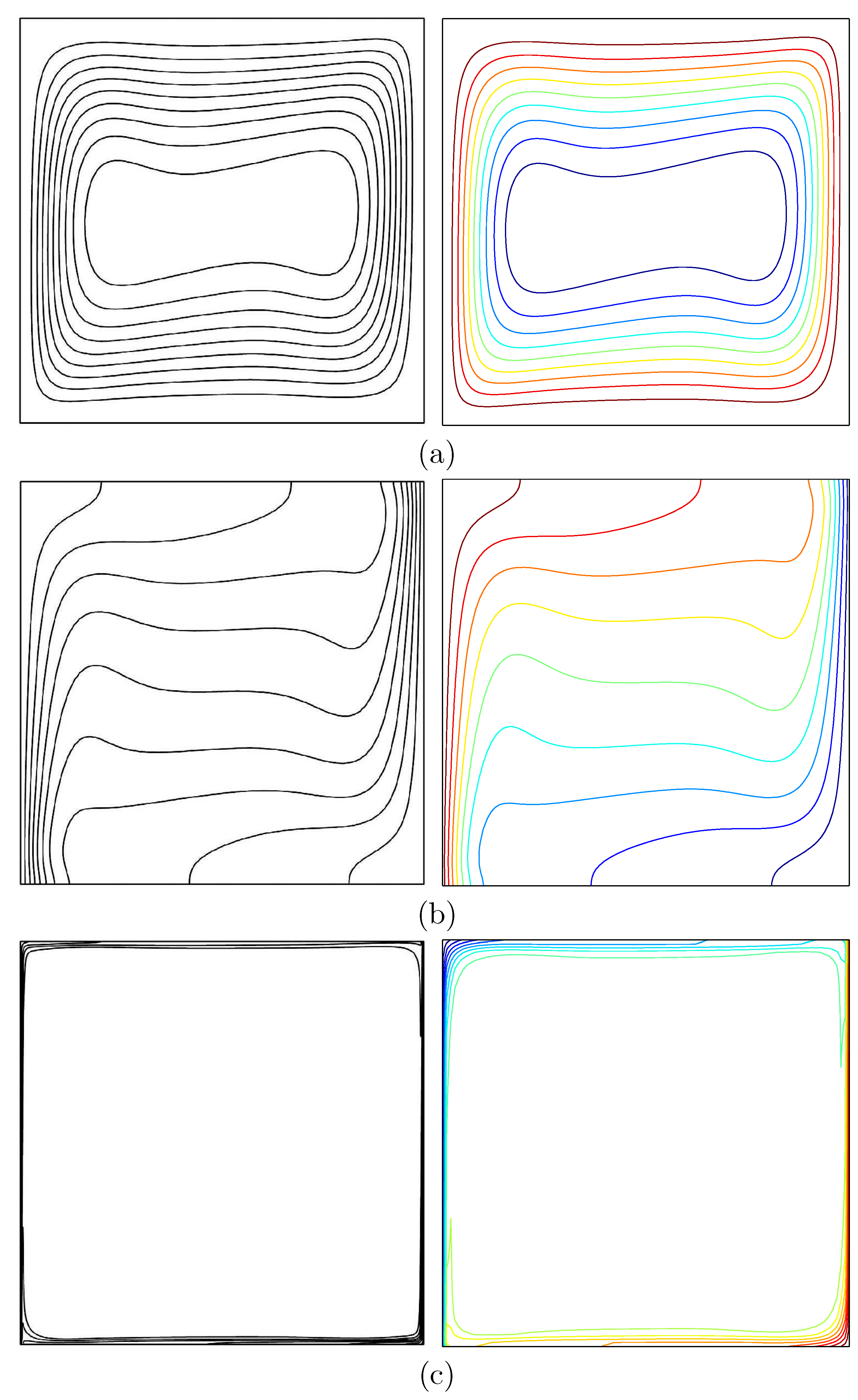
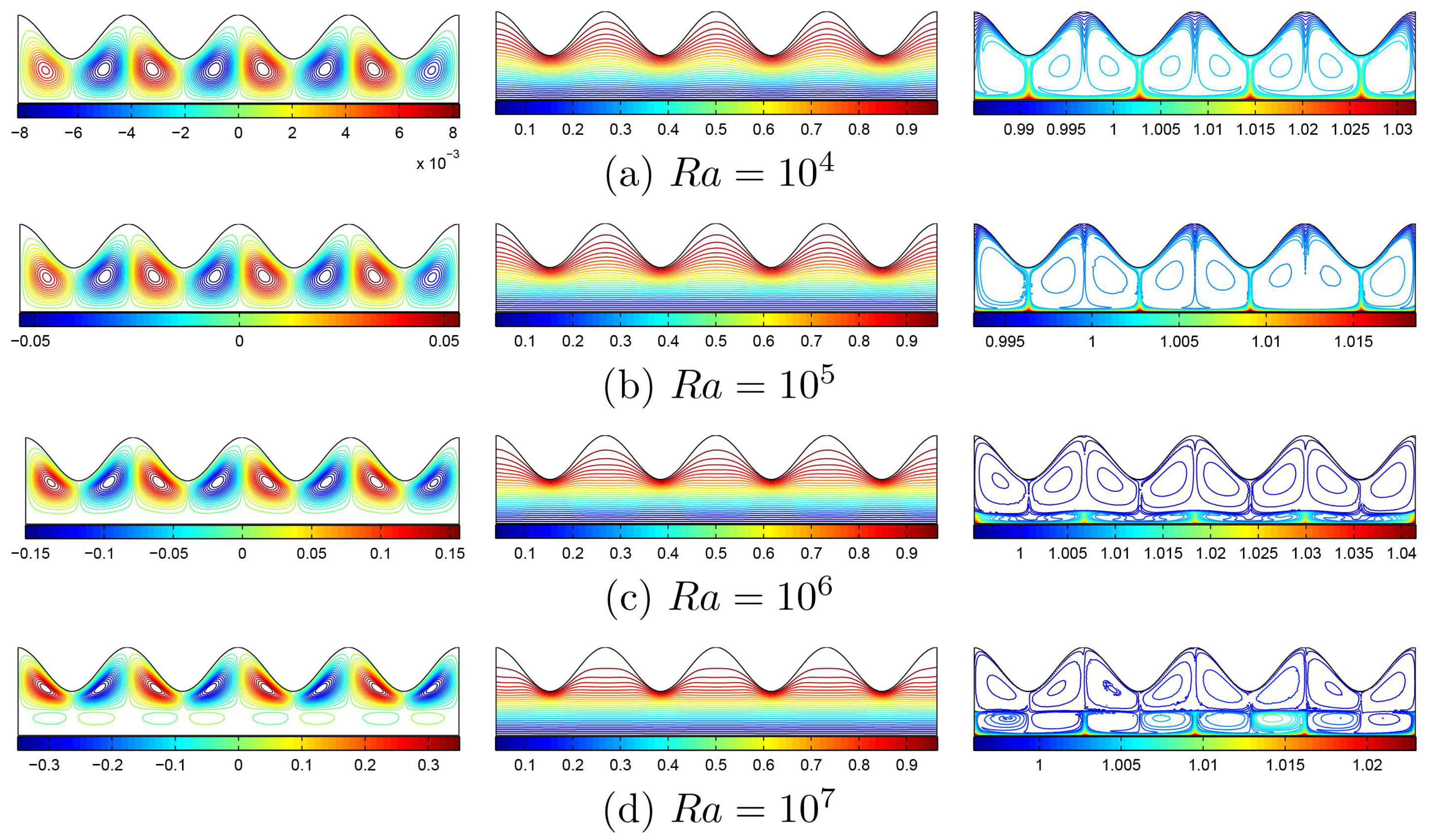
- At lower Rayleigh number values, conductive heat transfer is more dominant than the convective heat transfer. Moreover, improving the Rayleigh number leads to higher heat transfer due to the strong convection current.
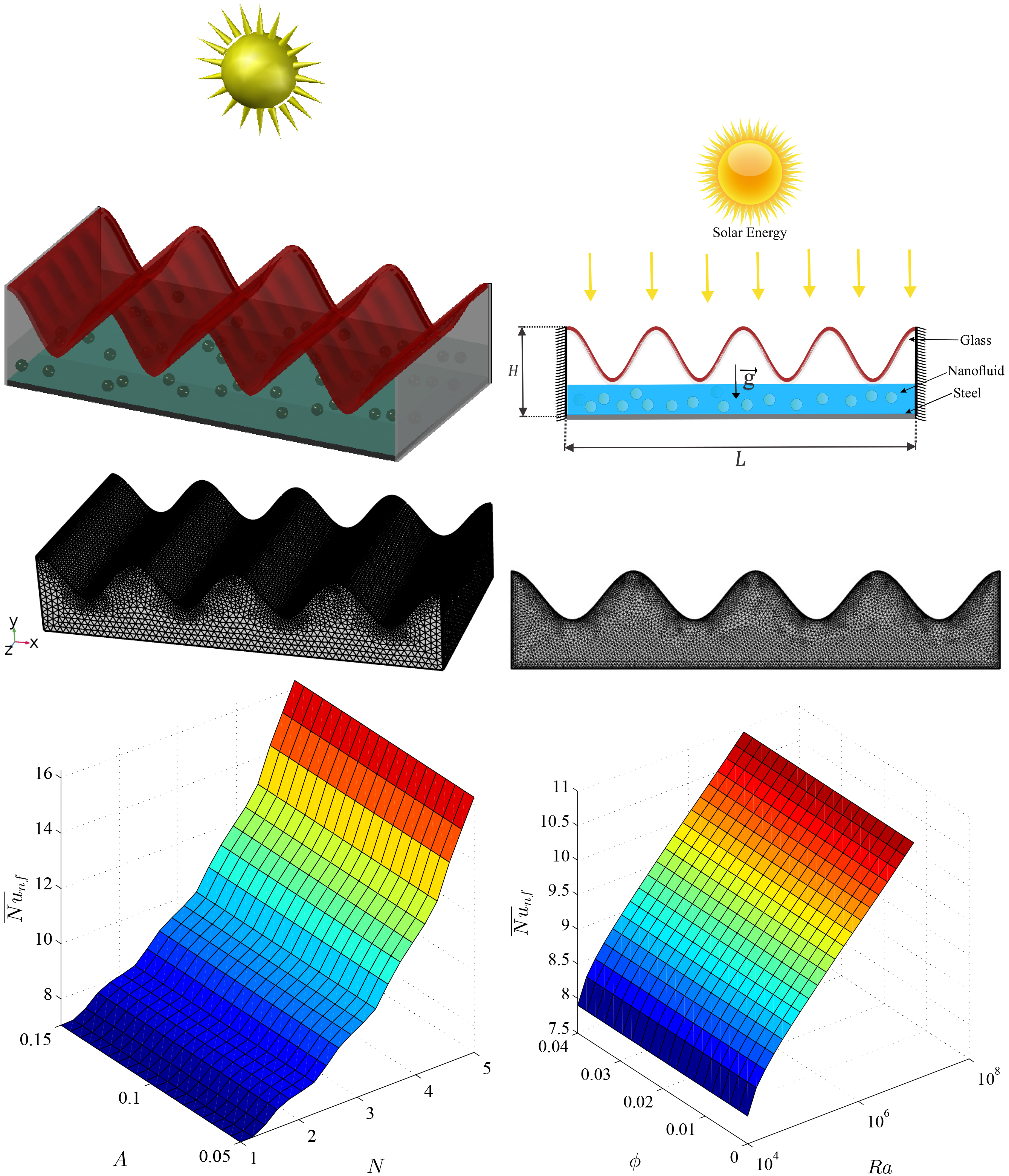
- The average Nusselt number develops upon raising both the wave amplitude and the number of oscillations. For both cases, growing the length of the wavy surface results in more energy transfer from the hot surface. More importantly, the heat transfer enhancement is observed more significantly with the variation of the wave amplitude.
- Augmentation of the nanoparticles concentration tends to boost the nanofluid thermal conductivity, and as a result, a gain in the average Nusselt number is obtained due to the higher thermal gradient and energy transport.
Author Contributions
Funding
Conflicts of Interest
Abbreviations
| Nomenclature | |
| A | amplitude |
| specific heat capacity | |
| diameter of the base fluid molecule | |
| diameter of the nanoparticle | |
| Brownian diffusion coefficient | |
| reference Brownian diffusion coefficient | |
| thermophoretic diffusivity coefficient | |
| reference thermophoretic diffusion coefficient | |
| H | thickness of solar collector |
| k | thermal conductivity |
| L | length of the solar collector |
| Lewis number | |
| N | number of oscillations |
| ratio of Brownian to thermophoretic diffusivity | |
| average Nusselt number | |
| Pr | Prandtl number |
| Rayleigh number | |
| Brownian motion Reynolds number | |
| S | total length of the wavy heater |
| Schmidt number | |
| T | temperature |
| reference temperature (310K) | |
| freezing point of the base fluid (273.15K) | |
| velocity vector | |
| normalized velocity vector | |
| Brownian velocity of the nanoparticle | |
| W | width of the solar collector |
| x, y, z & X, Y, Z | space coordinates & dimensionless space coordinates |
| Greek symbols | |
| thermal diffusivity | |
| inclination angle of magnetic field | |
| thermal expansion coefficient | |
| normalized temperature parameter | |
| dimensionless temperature | |
| dynamic viscosity | |
| kinematic viscosity | |
| density | |
| solid volume fraction | |
| normalized solid volume fraction | |
| average solid volume fraction | |
| Subscript | |
| c | cold |
| f | base fluid |
| h | hot |
| nanofluid | |
| p | solid nanoparticles |
References
- Ozturk, I.; Aslan, A.; Kalyoncu, H. Energy consumption and economic growth relationship: Evidence from panel data for low and middle income countries. Energy Policy 2010, 38, 4422–4428. [Google Scholar] [CrossRef]
- Liu, Z. Global Energy Interconnection; Academic Press: Oxford, MA, USA, 2015. [Google Scholar]
- Akhmat, G.; Zaman, K.; Shukui, T.; Sajjad, F.; Khan, M.A.; Khan, M.Z. The challenges of reducing greenhouse gas emissions and air pollution through energy sources: Evidence from a panel of developed countries. Environ. Sci. Pollut. Res. 2014, 21, 7425–7435. [Google Scholar] [CrossRef] [PubMed]
- Alper, A.; Oguz, O. The role of renewable energy consumption in economic growth: Evidence from asymmetric causality. Renew. Sustain. Energy Rev. 2016, 60, 953–959. [Google Scholar] [CrossRef]
- Al-Karaghouli, A.; Renne, D.; Kazmerski, L.L. Solar and wind opportunities for water desalination in the Arab regions. Renew. Sustain. Energy Rev. 2009, 13, 2397–2407. [Google Scholar] [CrossRef]
- Colangelo, G.; Milanese, M. Numerical simulation of thermal efficiency of an innovative Al2O3 nanofluid solar thermal collector: Influence of nanoparticles concentration. Therm. Sci. 2017, 21, 2769–2779. [Google Scholar] [CrossRef]
- Lewis, N.S. Toward cost-effective solar energy use. Science 2007, 315, 798–801. [Google Scholar] [CrossRef] [Green Version]
- Xu, B.; Xu, J.; Chen, Z. Heat transfer study in solar collector with energy storage. Int. J. Heat Mass Transf. 2020, 156, 119778. [Google Scholar] [CrossRef]
- Behura, A.K.; Gupta, H.K. Efficient direct absorption solar collector using banomaterial suspended heat transfer fluid. Mater. Today Proc. 2020, 22, 1664–1668. [Google Scholar] [CrossRef]
- Tian, Y.; Zhao, C.Y. A review of solar collectors and thermal energy storage in solar thermal applications. Appl. Energy 2013, 104, 538–553. [Google Scholar] [CrossRef] [Green Version]
- Liu, S.Y.; Perng, Y.H.; Ho, Y.F. The effect of renewable energy application on Taiwan buildings: What are the challenges and strategies for solar energy exploitation? Renew. Sustain. Energy Rev. 2013, 28, 92–106. [Google Scholar] [CrossRef]
- Elsheikh, A.H.; Elaziz, M.A. Review on applications of particle swarm optimization in solar energy systems. Int. J. Environ. Sci. Technol. 2019, 16, 1159–1170. [Google Scholar] [CrossRef]
- Minardi, J.E.; Chuang, H.N. Performance of a “black” liquid flat-plate solar collector. Sol. Energy 1975, 17, 179–183. [Google Scholar] [CrossRef]
- Otanicar, T.P.; Phelan, P.E.; Golden, J.S. Optical properties of liquids for direct absorption solar thermal energy systems. Sol. Energy 2009, 83, 969–977. [Google Scholar] [CrossRef]
- Milanese, M.; Colangelo, G.; Cretì, A.; Lomascolo, M.; Iacobazzi, F.; De Risi, A. Optical absorption measurements of oxide nanoparticles for application as nanofluid in direct absorption solar power systems—Part I: Water-based nanofluids behavior. Sol. Energy Mater. Sol. Cells 2016, 147, 315–320. [Google Scholar] [CrossRef]
- Milanese, M.; Colangelo, G.; Cretì, A.; Lomascolo, M.; Iacobazzi, F.; De Risi, A. Optical absorption measurements of oxide nanoparticles for application as nanofluid in direct absorption solar power systems—Part II: ZnO, CeO2, Fe2O3 nanoparticles behavior. Sol. Energy Mater. Sol. Cells 2016, 147, 321–326. [Google Scholar] [CrossRef]
- Pizzarelli, M. The status of the research on the heat transfer deterioration in supercritical fluids: A review. Int. Commun. Heat Mass Transf. 2018, 95, 132–138. [Google Scholar] [CrossRef]
- Duangthongsuk, W.; Wongwises, S. An experimental study on the heat transfer performance and pressure drop of TiO2-water nanofluids flowing under a turbulent flow regime. Int. J. Heat Mass Transf. 2010, 53, 334–344. [Google Scholar] [CrossRef]
- Iacobazzi, F.; Milanese, M.; Colangelo, G.; de Risi, A. A critical analysis of clustering phenomenon in Al2O3 nanofluids. J. Therm. Anal. Calorim. 2019, 135, 371–377. [Google Scholar] [CrossRef]
- Otanicar, T.P.; Phelan, P.E.; Prasher, R.S.; Rosengarten, G.; Taylor, R.A. Nanofluid-based direct absorption solar collector. J. Renew. Sustain. Energy 2010, 2, 033102. [Google Scholar] [CrossRef] [Green Version]
- Parvin, S.; Nasrin, R.; Alim, M.A. Heat transfer and entropy generation through nanofluid filled direct absorption solar collector. Int. J. Heat Mass Transf. 2014, 71, 386–395. [Google Scholar] [CrossRef]
- Gorji, T.B.; Ranjbar, A.A. Geometry optimization of a nanofluid-based direct absorption solar collector using response surface methodology. Sol. Energy 2015, 122, 314–325. [Google Scholar] [CrossRef]
- Potenza, M.; Milanese, M.; Colangelo, G.; de Risi, A. Experimental investigation of transparent parabolic trough collector based on gas-phase nanofluid. Appl. Energy 2017, 203, 560–570. [Google Scholar] [CrossRef]
- Gorji, T.B.; Ranjbar, A.A. A review on optical properties and application of nanofluids in direct absorption solar collectors (DASCs). Renew. Sustain. Energy Rev. 2017, 72, 10–32. [Google Scholar] [CrossRef]
- Fard, M.H.; Esfahany, M.N.; Talaie, M.R. Numerical study of convective heat transfer of nanofluids in a circular tube two-phase model versus single-phase model. Int. Commun. Heat Mass Transf. 2010, 37, 91–97. [Google Scholar] [CrossRef]
- Göktepe, S.; Atalık, K.; Ertürk, H. Comparison of single and two-phase models for nanofluid convection at the entrance of a uniformly heated tube. Int. J. Therm. Sci. 2014, 80, 83–92. [Google Scholar] [CrossRef]
- Mohyud-Din, S.T.; Zaidi, Z.A.; Khan, U.; Ahmed, N. On heat and mass transfer analysis for the flow of a nanofluid between rotating parallel plates. Aerosp. Sci. Technol. 2015, 46, 514–522. [Google Scholar] [CrossRef]
- Hayat, T.; Imtiaz, M.; Alsaedi, A.; Kutbi, M.A. MHD three-dimensional flow of nanofluid with velocity slip and nonlinear thermal radiation. J. Magn. Magn. Mater. 2015, 396, 31–37. [Google Scholar] [CrossRef]
- Hatami, M.; Khazayinejad, M.; Zhou, J.; Jing, D. Three-dimensional and two-phase nanofluid flow and heat transfer analysis over a stretching infinite solar plate. Therm. Sci. 2018, 22, 871–884. [Google Scholar] [CrossRef] [Green Version]
- Nasrin, R.; Alim, M.A. Performance of nanofluids on heat transfer in a wavy solar collector. Int. J. Eng. Sci. Technol. 2013, 5, 58–77. [Google Scholar] [CrossRef] [Green Version]
- Hatami, M.; Jing, D. Optimization of wavy direct absorber solar collector (WDASC) using Al2O3-water nanofluid and RSM analysis. Appl. Therm. Eng. 2017, 121, 1040–1050. [Google Scholar] [CrossRef]
- Hatami, M.; Jing, D. Evaluation of wavy direct absorption solar collector (DASC) performance using different nanofluids. J. Mol. Liq. 2017, 229, 203–211. [Google Scholar] [CrossRef]
- Buongiorno, J. Convective transport in nanofluids. J. Heat Transf. 2006, 128, 240–250. [Google Scholar] [CrossRef]
- Alsabery, A.I.; Gedik, E.; Chamkha, A.J.; Hashim, I. Effects of two-phase nanofluid model and localized heat source/sink on natural convection in a square cavity with a solid circular cylinder. Comput. Methods Appl. Mech. Eng. 2019, 346, 952–981. [Google Scholar] [CrossRef]
- Corcione, M. Empirical correlating equations for predicting the effective thermal conductivity and dynamic viscosity of nanofluids. Energy Convers. Manag. 2011, 52, 789–793. [Google Scholar] [CrossRef]
- Alsabery, A.; Armaghani, T.; Chamkha, A.; Hashim, I. Conjugate heat transfer of Al2O3–water nanofluid in a square cavity heated by a triangular thick wall using Buongiorno’s two-phase model. J. Therm. Anal. Calorim. 2019, 135, 161–176. [Google Scholar] [CrossRef]
- Corcione, M.; Cianfrini, M.; Quintino, A. Two-phase mixture modeling of natural convection of nanofluids with temperature-dependent properties. Int. J. Therm. Sci. 2013, 71, 182–195. [Google Scholar] [CrossRef]
- Putra, N.; Roetzel, W.; Das, S.K. Natural convection of nano-fluids. Heat Mass Transf. 2003, 39, 775–784. [Google Scholar] [CrossRef]
- Chon, C.H.; Kihm, K.D.; Lee, S.P.; Choi, S.U. Empirical correlation finding the role of temperature and particle size for nanofluid (Al2O3) thermal conductivity enhancement. Appl. Phys. Lett. 2005, 87, 3107. [Google Scholar] [CrossRef]
- Ho, C.; Liu, W.; Chang, Y.; Lin, C. Natural convection heat transfer of alumina-water nanofluid in vertical square enclosures: An experimental study. Int. J. Therm. Sci. 2010, 49, 1345–1353. [Google Scholar] [CrossRef]
- Bergman, T.L.; Incropera, F.P. Introduction to Heat Transfer, 6th ed.; Wiley: New York, NY, USA, 2011. [Google Scholar]


| Physical Properties | Fluid Phase (Water) | AlO |
|---|---|---|
| 0.628 | 40 | |
| 695 | – | |
| 993 | 3970 | |
| 4178 | 765 | |
| 36.2 | 0.85 | |
| 0.385 | 33 |
Publisher’s Note: MDPI stays neutral with regard to jurisdictional claims in published maps and institutional affiliations. |
© 2020 by the authors. Licensee MDPI, Basel, Switzerland. This article is an open access article distributed under the terms and conditions of the Creative Commons Attribution (CC BY) license (http://creativecommons.org/licenses/by/4.0/).
Share and Cite
Alsabery, A.I.; Parvin, S.; Ghalambaz, M.; Chamkha, A.J.; Hashim, I. Convection Heat Transfer in 3D Wavy Direct Absorber Solar Collector Based on Two-Phase Nanofluid Approach. Appl. Sci. 2020, 10, 7265. https://0-doi-org.brum.beds.ac.uk/10.3390/app10207265
Alsabery AI, Parvin S, Ghalambaz M, Chamkha AJ, Hashim I. Convection Heat Transfer in 3D Wavy Direct Absorber Solar Collector Based on Two-Phase Nanofluid Approach. Applied Sciences. 2020; 10(20):7265. https://0-doi-org.brum.beds.ac.uk/10.3390/app10207265
Chicago/Turabian StyleAlsabery, Ammar I., Salma Parvin, Mohammad Ghalambaz, Ali J. Chamkha, and Ishak Hashim. 2020. "Convection Heat Transfer in 3D Wavy Direct Absorber Solar Collector Based on Two-Phase Nanofluid Approach" Applied Sciences 10, no. 20: 7265. https://0-doi-org.brum.beds.ac.uk/10.3390/app10207265