World Ocean Thermocline Weakening and Isothermal Layer Warming

Abstract

This paper identifies world thermocline weakening and provides an improved estimate of upper ocean warming through replacement of the upper layer with the fixed depth range by the isothermal layer, because the upper ocean isothermal layer (as a whole) exchanges heat with the atmosphere and the deep layer. Thermocline gradient, heat flux across the air–ocean interface, and horizontal heat advection determine the heat stored in the isothermal layer. Among the three processes, the effect of the thermocline gradient clearly shows up when we use the isothermal layer heat content, but it is otherwise when we use the heat content with the fixed depth ranges such as 0–300 m, 0–400 m, 0–700 m, 0–750 m, and 0–2000 m. A strong thermocline gradient exhibits the downward heat transfer from the isothermal layer (non-polar regions), makes the isothermal layer thin, and causes less heat to be stored in it. On the other hand, a weak thermocline gradient makes the isothermal layer thick, and causes more heat to be stored in it. In addition, the uncertainty in estimating upper ocean heat content and warming trends using uncertain fixed depth ranges (0–300 m, 0–400 m, 0–700 m, 0–750 m, or 0–2000 m) will be eliminated by using the isothermal layer. The isothermal layer heat content with the monthly climatology removed (i.e., relative isothermal layer heat content) is calculated for an individual observed temperature profile from three open datasets. The calculated 1,111,647 pairs of (thermocline gradient, relative isothermal layer heat content) worldwide show long-term decreasing of the thermocline gradient and increasing of isothermal layer heat content in the global as well as regional oceans. The global ocean thermocline weakening rate is (−2.11 ± 0.31) × 10⁻³ (°C m⁻¹ yr⁻¹) and isothermal layer warming rate is (0.142 ± 0.014) (W m⁻²).

1. Introduction

The thermocline with a strong vertical gradient is the transition layer between the vertically quasi-uniform layer from the surface, the isothermal layer (ITL), and the deep-water layer [1,2]. Intense turbulent mixing near the ocean surface causes formation of ITL. The thermocline resists the turbulent mixing from the ITL and limits the ITL deepening and heat exchange between the ITL and deeper layer due to its strong vertical gradient. The mean thermocline gradient (G) directly affects the ITL warming or cooling [3,4,5,6].

The oceanic climate change is represented by temporal variation of the upper layer ocean heat content (OHC), which is the integrated heat stored in the layer from the sea surface (z = 0) down to a below-surface depth. Here, z is the vertical coordinate. The below-surface depth can be either a fixed depth or the ITL depth (h). With h as the below-surface depth, the upper layer OHC is called the ITL heat content (H_ITL). Both G and H_ITL are important in ocean prediction [6].

However, the oceanographic community uses various fixed depths to define the OHC such as 0–300 m [7,8], 0–400 m [9], 0–700 m [10,11], 0–750 m [12], 0–2000 m [13], deep layer OHC such as below 700 m [8], and below 2000 m [14], and the full layer OHC [15]. We apologize for not citing all the work on the ocean OHC due to the huge amount of literature. Interested readers are referred to two excellent review papers [16,17].

Such fixed-depth OHC has three weaknesses. First, the layer with the fixed depth range includes ITL, the thermocline, and the layer below the thermocline. The effects of the thermocline gradient on ocean climate change and phytoplankton dynamics are not represented. Phytoplankton growth depends upon water temperature, light, and availability of nutrients. Nutrients are normally brought up from deep waters and into the photic zone where phytoplankton growth can occur [18]. Such nutrient pumping is affected by the thermocline gradient. Second, the fixed-depth OHC leads to the uncertainty in estimating the upper ocean warming trend. For example, the warming trend is estimated as 0.64 ± 0.11 W m⁻² for OHC (0–300 m) on 1993–2008 with the significant level α = 0.10 [8], 0.26 ± 0.02 W m⁻² for OHC (0–300 m) on 1975–2009 [14] and 0.20 W m⁻² for OHC (0–700 m) on 1955–2012 [10], among others (see

Table 1. Several reported trends (warming rate) of fixed depth ocean heat content anomaly.

Source	Fixed-Depth Layer	Trend (W m−2)	Duration
Lyman and Johnson (2014) [11]	H0–100 m	0.07	1956–2011
Lyman and Johnson (2014) [11]	H0–100 m	0.10	1967–2011
Lyman and Johnson (2014) [11]	H0–100 m	0.09	1983–2011
Lyman and Johnson (2014) [11]	H0–100 m	−0.04	2004–2011
Lyman et al. (2010) [8]	H0–300 m	0.64 ± 0.11	1993–2008
Lyman and Johnson (2014) [11]	H0–300 m	0.19	1967–2011
Lyman and Johnson (2014) [11]	H0–300 m	0.25	1983–2011
Lyman and Johnson (2014) [11]	H0–300 m	0.10	2004–2011
Balmaseda et al. (2013) [14]	H0–300 m	0.26 ± 0.02	1975–2009
Balmaseda et al. (2013) [14]	H0–700 m	0.38 ± 0.03	1975–2009
Levitus et al. (2012) [10]	H0–700 m	0.27	1955–2010
Lyman and Johnson (2014) [11]	H0–700 m	0.43	1983–2011
Lyman and Johnson (2014) [11]	H0–700 m	0.13	2004–2011
Willis et al. (2003) [12]	H0–750 m	0.86 ± 0.12	1993–2003
Lyman and Johnson (2014) [11]	H0–1800 m	0.29	2004–2011
Levitus et al. (2012) [10]	H0–2000 m	0.39	1955–2010
Zanna et al. (2019) [13]	H0–2000 m	0.30 ± 0.6	1955–2017

). Third, there is no simple relationship between the OHC with the fixed depth range and the sea surface temperature, which is the most important oceanic variable for the heat exchange between the ocean and atmosphere.

Alternatively, we use the ITL OHC (H_ITL) to overcome these three weaknesses of the traditional OHC with the fixed depth range. Recently, a global ocean synoptic thermocline gradient (G) and isothermal layer depth (h) dataset has been established from the NOAA/NCEI World Ocean Database (WOD) with each (G, h) pair corresponding to particular CTD (or XBT) temperature profile in WOD [19,20]. This synoptic dataset is at the NOAA website (https://www.ncei.noaa.gov/access/metadata/landing-age/bin/iso?id=gov.noaa.nodc:0173210) for public use. With the given ITL depth h, it is easy to compute ITL heat content (H_ITL). After the quality control, we have 1,111,647 (G, H_ITL) data pairs for the global oceans. The warming trend can be identified from the H_ITL data. A new phenomenon ‘thermocline weakening’ was explored.

2. Data

Three open datasets were used for this study. The first one is the NOAA World Ocean Database 2018 (WOD18) conductivity, temperature, depth (CTD) and expendable bathythermograph (XBT) temperature profiles T(t, r, z) 1970–2017 (https://www.nodc.noaa.gov/OC5/WOD/pr_wod.html) [19]. Here, the Earth coordinate system is used with r = (x, y) for the longitudinal and latitudinal and z in the vertical (upward positive). The second one is the 0.25° × 0.25° gridded climatological monthly mean temperature fields ${\widehat{T}}_c(t_c,r_c,z_c)$ of the NOAA World Ocean Atlas 2018 (WOA18) (https://www.nodc.noaa.gov/OC5/woa18/) [20] with t_c representing the month, r_c the horizontal grid point, and z_c the WOA standard depth. The third one is the global ocean thermocline gradient, ITL depth, and other upper ocean parameters calculated from WOD CTD and XBT temperature profiles from 1 January1970 to 31 December 2017 (NCEI Accession 0173210) (https://data.nodc.noaa.gov/cgi-bin/iso?id=gov.noaa.nodc:0173210) [21], which was established using the optimal schemes [22,23,24]. The third dataset contains 1,202,061 synoptic G(t, r) and h(t, r) for the world oceans [25]. Each data pair has a corresponding observed temperature profile T(t, r, z) in the first dataset.

The decadal variations of statistical parameters for the global (G, h) data are depicted in

Table 2. Decadal variation of statistical characteristics of the global isothermal layer depth (h) in comparison to climatology.

	Mean (m)	Standard Deviation (m)	Skewness	Kurtosis
1970–1980	38.8	41.7	3.97	27.3
1981–1990	55.0	54.6	3.22	21.0
1991–2000	62.8	58.0	2.95	18.4
2001–2010	66.3	61.5	2.82	17.0
2011–2017	67.5	61.7	2.70	15.1

(isothermal layer depth h) and

Table 3. Decadal variation of statistical characteristics of the global thermocline gradient (G) in comparison to climatology.

	Mean (°C/m)	Standard Deviation (°C/m)	Skewness	Kurtosis
1970–1980	0.204	0.167	1.35	5.02
1981–1990	0.162	0.150	1.77	6.61
1991–2000	0.130	0.133	2.29	9.47
2001–2010	0.124	0.132	2.35	9.69
2011–2017	0.121	0.134	2.55	10.90

(thermocline gradient G). Both (h, G) are positively skewed. The isothermal layer depth (h) monotonically increased its mean (standard deviation) from 38.8 m (41.7 m) during 1970–1980 to 67.5 m (61.7 m) during 2011–2017, and monotonically decreased skewness (kurtosis) from 3.97 (27.3) during 1970–1980 to 2.70 (15.1) during 2011–2017. The thermocline gradient (G) monotonically decreased its mean (standard deviation) from 0.204 °C/m (0.167 °C/m) during 1970–1980 to 0.121 °C/m (0.134 °C/m) during 2011–2017, and increased its skewness (kurtosis) from 1.35 (5.02) during 1970–1980 to 2.55 (10.9) during 2011–2017. Interested readers are referred to the reference [25].

3. Methods

3.1. Describing Mixed Layer Dynamics

The connection between G (unit: °C m⁻¹) and the ITL heat content H_ITL (unit: J m⁻²) can be found using the conservation of heat in the ITL [1,3,4,5,26]

$$\begin{array}{l}{H}_{ITL}={\rho }_0{c}_{p}h{T}_I\\ \frac{\partial T_I}{\partial t}=-v•\nabla T_I-\frac{Q}{{\rho }_0{c}_{p}h}-\mathsf{\Lambda }\frac{w_e}{h}\Delta T,\Delta T\equiv T_I(t,r)-T_{th}(t,r)\end{array}$$

(1)

where v (unit: m s⁻¹)is the bulk ITL horizontal velocity vector; h is the isothermal layer depth (unit: m); T_I is the ITL temperature (unit: °C); Q (unit: W m⁻²) is the net heat flux at the ocean surface (upward positive); w_e (unit: m s⁻¹) is the entrainment velocity; Λ is the step function taking 0 if w_e < 0, and 1 otherwise due to the second law of the thermodynamics; ΔT is the temperature difference between ITL and thermocline; T_th(t, r) is the thermocline temperature (unit: °C). It is reasonable to assume that the temperature difference is proportional to the thermocline gradient, ΔT = γG, with the proportionality γ (unit: m). Using conservation of mass in the ITL gives the H_ITL equation

$$\frac{\partial H_{ITL}}{\partial t}=-v•\nabla H_{ITL}-{\rho }_0{c}_{p}hv•\nabla {\widehat{T}}_I-{\rho }_0{c}_p\left(T_I-{\widehat{T}}_I\right)w_{-h}-Q-\mathsf{\Lambda }{\rho }_0{c}_p{w}_e\left[\gamma G-\left(T_I-{\widehat{T}}_I\right)\right]$$

(2)

where ${\widehat{T}}_I$ is the temperature below the ITL; the last term in the right-hand side of (2) occurs only the mixed layer dynamics and thermodynamics are included. For the entrainment regime (w_e > 0, Λ = 1), the thermocline gradient G is related negatively to ∂H_ITL/∂t. Strong (weak) thermocline gradient causes the decrease (increase) in H_ITL. Such an entrainment effect does not show up with the upper ocean heat content with fixed depth ranges commonly used in oceanography such as 0–300 m, 0–400 m, 0–700 m, 0–750 m, and 0–2000 m.

3.2. Methodological Procedure

For each observational CTD/XBT temperature profile T(t, r, z) from the first dataset WOD18 [22], a pair of [G(t, r), h(t, r)] is identified from the third dataset with the same time t and horizontal location r. We use the 3D linear interpolation to calculate a climatological profile ${\widehat{T}}_c(r,z)$ at the observational location (r, z) from four neighboring grid points of the temperature field ${\widehat{T}}_c(t_c,r_c,z_c)$ from the second dataset WOA18 [23] for the same month.

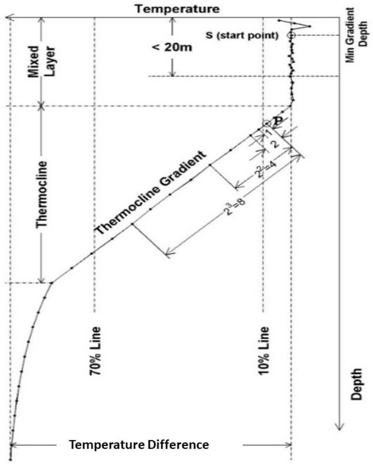
The ITL depth (h) was determined from an individual temperature profile using the optimal fitting and exponential leap-forward gradient scheme (Figure 1). It contains four steps: (1) estimating the ITL gradient (near-zero), (2) identifying the thermocline gradient G, (3) computing the vertical gradient at each depth (non-dimensionalized by G), and (4) determining h with a given threshold (or user input) to separate the near-zero gradient layer (i.e., the ITL) and the non-zero gradient layer (i.e., the thermocline). Figure 1 illustrates the procedures of this method. Interested readers are referred to [22,23,24] for detailed information.

For an observational temperature profile T(t, r, z) the corresponding climatological monthly mean profile $\widehat{T}(r,z)$ is obtained. With h(t, r), we calculate the difference $\left[T(t,r,z)-\widehat{T}(r,z)\right]$ first and then the ITL heat content (H_ITL) with the mean monthly variation removed (i.e., relative ITL heat content),

$$H_{ITL}(t,r)=c_p{\rho }_0{\displaystyle \underset{-h(t,r)}{\overset{0}{\int }}\left[T(t,r,z)-\widehat{T}(r,z)\right]dz}$$

(3)

where c_p = 3985 J kg⁻¹ °C⁻¹ is the specific heat for sea water; ρ₀ = 1025 kg m⁻³ is the upper ocean characteristic density. Let

$$T_I(t,r)\equiv \frac{1}{h}{\displaystyle \underset{-h(t,r)}{\overset{0}{\int }}T(t,r,z)dz},{\widehat{T}}_I(r)\equiv \frac{1}{h}{\displaystyle \underset{-h(t,r)}{\overset{0}{\int }}\widehat{T}(r,z)dz}$$

(4)

be the in-situ and corresponding climatological monthly ITL temperature. With (3) and (4), we have

$$H_{ITL}(t,r)={\rho }_0{c}_{p}h(t,r)\left[T_I(t,r)-{\widehat{T}}_I(r)\right]$$

(5)

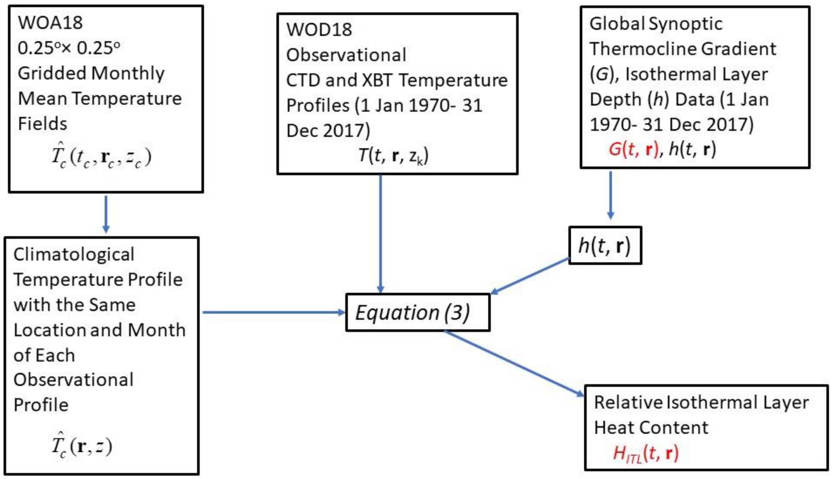
After quality control, we have 1,111,647 data pairs of [H_ITL(t, r), G(t, r)] for the global oceans from 1 January 1970 to 31 December 2017. Such a procedure to get the data pairs of [H_ITL(t, r), G(t, r)] is depicted in the flow chart (Figure 2).

3.3. Time Series of (H_ITL, G) for Global and Regional Oceans

To further explore the temporal variability for global and regional oceans, we represent 1,111,647 (H_ITL, G) pairs into the format of [H_ITL(m, τ_i, r_j), G(m, τ_i, r_j)] with m = 1, 2, …, 12 the time sequence in months; and τ_i = 1970, 1971, …, 2017 the time sequence in years with i = 1, 2, ..., N (N = 48), then we divide the world oceans excluding the Arctic Ocean into 12 regions (see the first column in

Table 4. Trends of H_ITL and G for different parts of world oceans.

Ocean	Number of Data	∂HITL/∂τ (W/m2)	∂G/∂τ [10−3 °C/(m × yr)]
Global Oceans	1,111,647	0.142 ± 0.014	−2.11 ± 0.31
North Atlantic (10° N–60° N)	335,747	0.128 ± 0.022	−1.49 ± 0.046
Equatorial Atlantic (10° S–10° N)	42,599	0.154 ± 0.036	−2.28 ± 0.58
South Atlantic (10° S–60° S)	57,540	0.0824 ± 0.04	−2.43 ± 0.73
Indian Ocean	150,789	0.160 ± 0.028	−2.77 ± 0.49
Equatorial Pacific (10° S–10° N)	89,924	0.156 ± 0.066	−3.51 ± 0.63
Southern Ocean (South of 60° S)	7942	−0.0272 ± 0.027	−1.19 ± 1.6
Western North Pacific
(10° N–60° N, 120° E–160° E)	101,447	0.139 ± 0.04	−2.07 ± 0.55
Central North Pacific
(10° N–60° N, 160° E–140° W)	88,967	0.135 ± 0.028	−1.65 ± 0.44
Eastern North Pacific
(10° N–60° N, 140° W–85° W)	91,572	0.104 ± 0.062	−2.05 ± 0.43
Western South Pacific
(10° S–60° S, 145° E–170° W)	79,472	0.140 ± 0.037	−0.821 ± 0.19
Central South Pacific
(10° S–60° S, 170° W–120° W)	23,632	0.125 ± 0.045	−0.378 ± 0.3
Eastern South Pacific
(10° S–60° S, 120° W–70° W)	16,965	0.005 ± 0.084	−1.61 ± 1.10

), and average the synoptic data pairs (H_ITL, G) within each region and the year to obtain 13 time-series of [<H_ITL(τ_i)>, <G(τ_i)>], including global ocean, with the time increment of a year. Differences among the 13 time-series shows the spatial variability of the yearly variation.

The trends of the time series are determined using linear regression (taking <G(τ_i)> for illustration),

$$\langle \widehat{G}(\tau )\rangle =a+b\tau ,\hspace{1em}b=\frac{\partial \langle \widehat{G}(\tau )\rangle }{\partial \tau }$$

(6)

The trend b is calculated from the data <G(τ_i)>,

$$b=\frac{S_{G\tau }}{S_{\tau \tau }},S_{\tau \tau }={\displaystyle \sum _{i=1}^N{({\tau }_i-\overline{\tau })}^2}, S_{GG}={\displaystyle \sum _{i=1}^N{(\langle G_i\rangle -\langle \overline{G}\rangle )}^2}, S_{G\tau }={\displaystyle \sum _{i=1}^N(\langle G_i\rangle -\langle \overline{G}\rangle )({\tau }_i-\overline{\tau })},$$

(7)

where

$$N=48,\langle G_i\rangle =\langle G({\tau }_i)\rangle ,\overline{\tau }=\frac{1}{N}{\displaystyle \sum _{i=1}^N{\tau }_i}, \langle \overline{G}\rangle =\frac{1}{N}{\displaystyle \sum _{i=1}^N\langle G_i\rangle }$$

(8)

The error in determining the trend b is estimated by the t-test. For a given significance level α, the confidence interval for the real trend $\widehat{b}$ is given by

$$b-t_{\alpha /2}\frac{S}{\sqrt{S_{\tau \tau }}}<\widehat{b}<b+t_{\alpha /2}\frac{S}{\sqrt{S_{\tau \tau }}},S^2=\frac{S_{GG}-b{S}_{G\tau }}{N-2}$$

(9)

where $t_{\alpha /2}$ is a value of the t distribution with (N − 2) degrees of freedom.

4. Results and Discussions

4.1. Decadal Variability of Global (H_ITL, G)

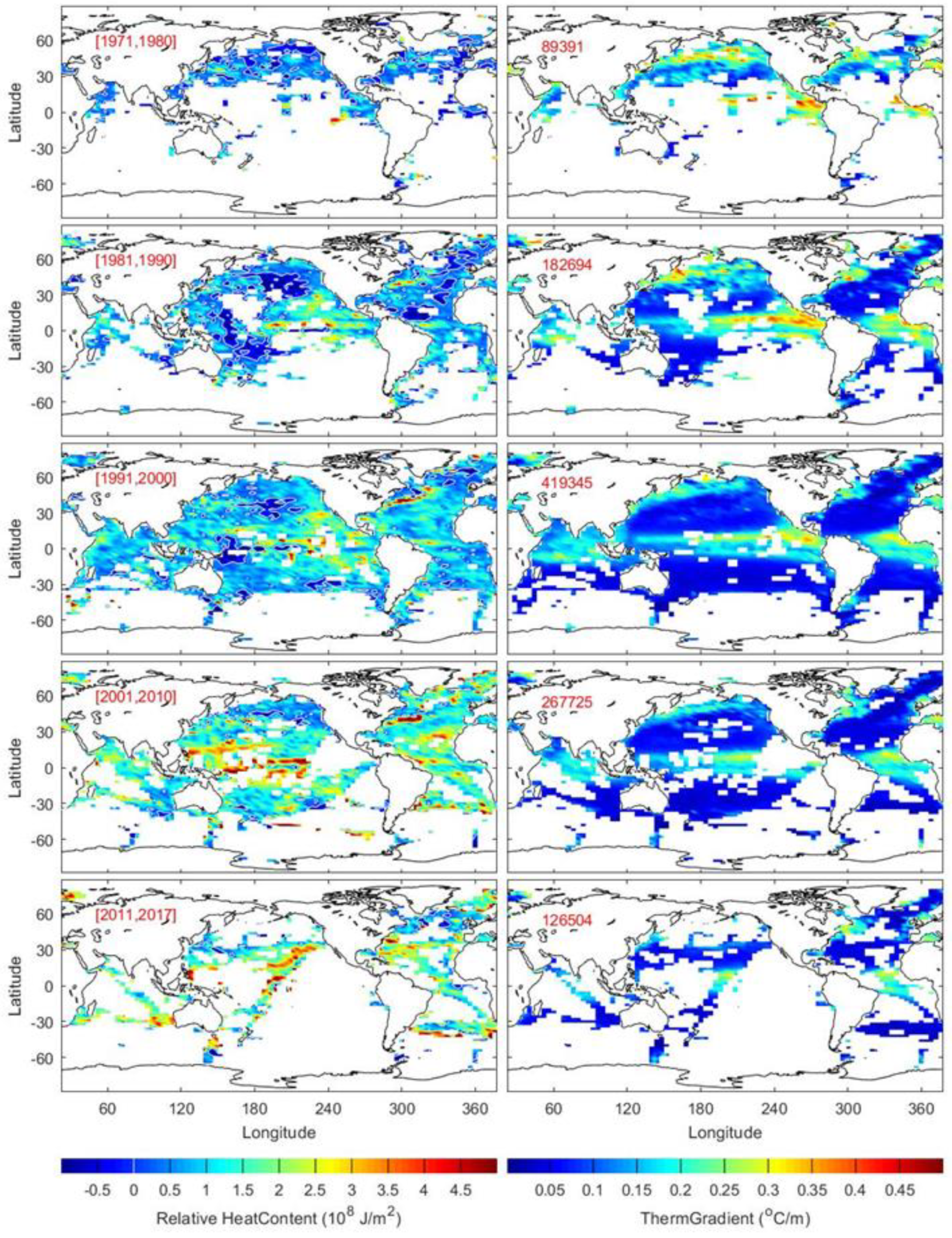
In analyzing global spatial and temporal variability, we divided the 1,111,647 synoptic data pairs of [H_ITL(t, r), G(t, r)] into six temporal periods: 1971–1980, 1981–1990, 1991–2000, 2001–2010, 2011–2017. For each time-period, we average the (H_ITL, G) data in 4° (longitude) × 2° (latitude) cell if the number of data pairs is larger than 5, and identify the cell with no data if the number of data pairs is less than 5. Figure 3 shows decadal variations of the global distributions of (H_ITL, G). The number of data points are on the right panels. The white grid cells denote no data or a number of data pairs less than 5. The most striking features are thermocline weakening and ITL warming. A strong thermocline gradient (G > 0.3 °C/m) occupied a vast area of the middle to high latitudes (north of 30° N) of the Northern Hemisphere as well as the eastern equatorial Pacific and Atlantic Oceans during 1971–1980, and 1981–1990. Such strong thermocline areas shrank during 1991–2000, and almost disappeared in 2011–2017. However, H_ITL increased steadily from 1971–1980 to 2011–2017. There was no area with H_ITL of more than 2.5 × 10⁸ J/m² in the middle to high latitudes of the Northern Hemisphere during 1971–1980. Warm areas (H_ITL > 2.5 × 10⁸ J/m²) showed up in these latitudes especially the western North Atlantic Ocean and equatorial Pacific and Atlantic Oceans in 1981–1990. The warm areas increased in 1991–2000, 2001–2010, and 2011–2017.

4.2. Trends of (H_ITL, G) for Global and Regional Oceans

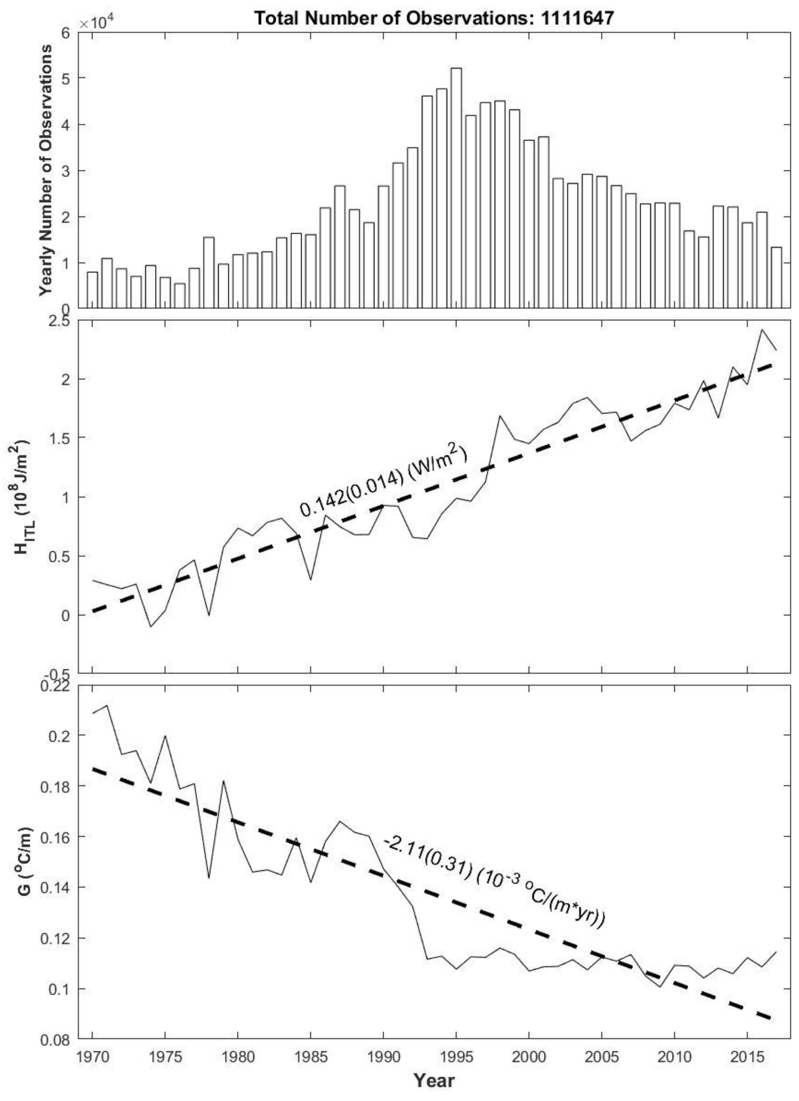
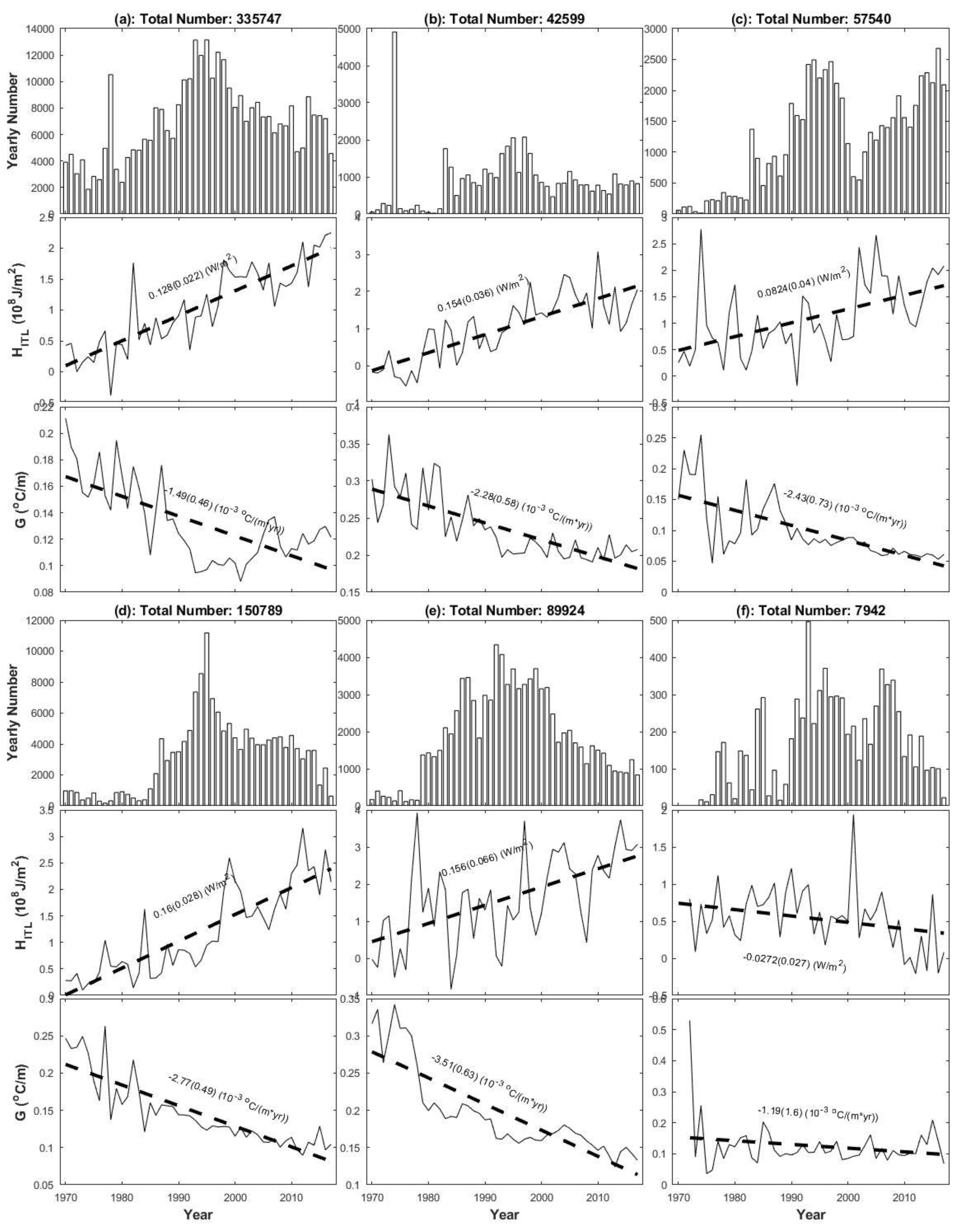
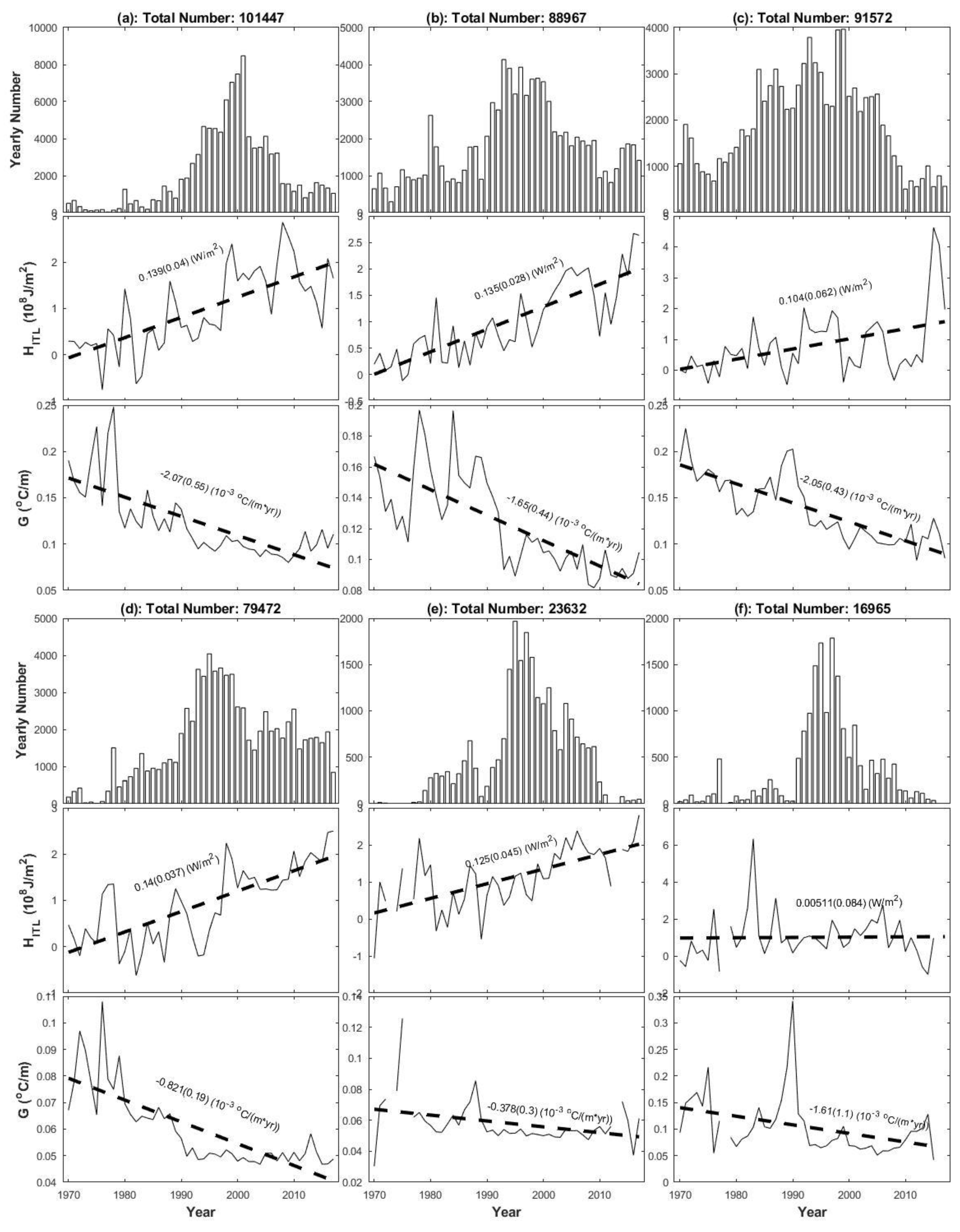
The 13 time series pairs [<H_ITL(τ_i)>, <G(τ_i)>] show the overall temporal (yearly) variability for the global and individual regional ocean. The significant level to estimate the trend of the time series is set as α = 0.05. The trends of G are all negative (i.e., ∂G/∂τ < 0) in the global ocean [(−2.11 ± 0.31) × 10⁻³ °C/(m × yr)] (Figure 4) as well as in all the 12 regions (Figure 5 and Figure 6). For regional oceans, the maximum weakening rate is [(−3.51 ± 0.63) × 10⁻³ °C/(m × yr)], occurring in the equatorial Pacific (10° S–10° N). The minimum weakening rate is [(−0.378 ± 0.3) × 10⁻³ °C/(m × yr)], appearing in the central South Pacific (10° S–60° S, 170° W–120° W). The trends of H_ITL are positive (i.e., ∂H_ITL/∂τ > 0) in the global ocean [0.142 ± 0.014 W/m²] (Figure 4) as well as in the 12 regions (Figure 5 and Figure 6) except the Southern Ocean. The maximum warm rate is (0.160 ± 0.028 W/m²), occurring in the Indian Ocean. The warm rate in the Equatorial Pacific (10° S–10° N) is also high (0.156 ± 0.066 W/m²).

The robust weakening trend of the thermocline gradient (∂G/∂τ < 0) and the warming trend of the isothermal layer (∂H_ITL/∂τ > 0) are found in global and regional oceans except the Southern Ocean, where slightly decreasing in the relative heat content (−0.0272 W m⁻²). The data are very sparse in the Southern Ocean with a total number of observations of 7942 (Figure 3, Figure 5f, and Table 4) and make the trends in the Southern Ocean not robust. The highest warming rate (0.160 ± 0.028 W m⁻²) of H_ITL in the Indian Ocean (Table 4) is coherent with the recent results on the fastest rate of warming in the tropical Indian Ocean among tropical oceans [27].

4.3. Comparison in the OHC Calculation between the Isothermal Layer and Fixed-Depth Layer

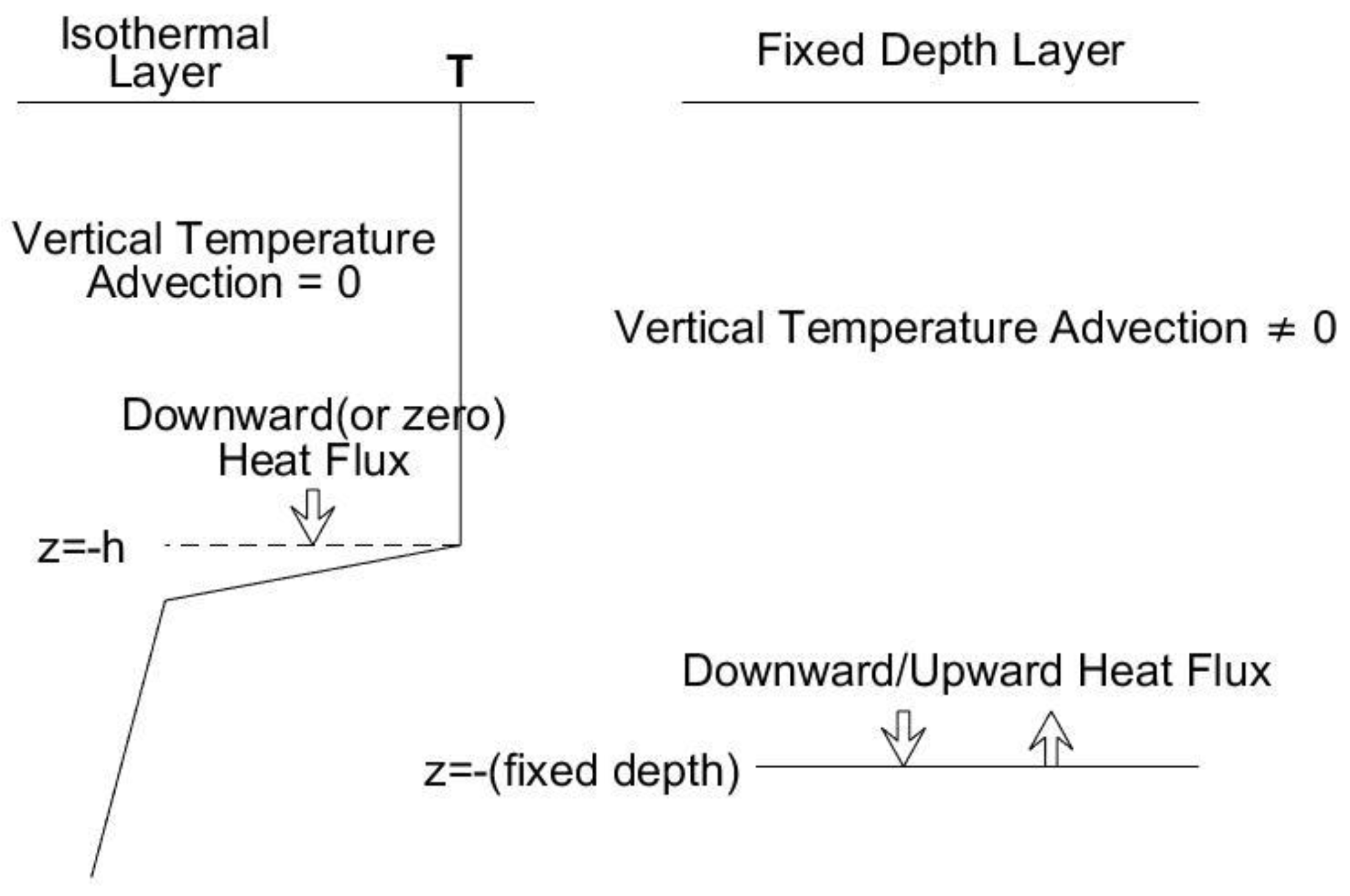
The dynamical characteristics are different between the isothermal layer and fixed-depth layer (Figure 7). In the isothermal layer, the vertical velocity does not cause the temperature advection since the vertical temperature gradient is near zero. The turbulent heat flux at the base of the mixed layer (z = −h) is downward or zero [3,4,5]. However, such simple dynamic features do not exist in the fixed-depth layer (0–100 m, 0–300 m, or 0–700 m), where the vertical temperature advection is not zero. The heat flux at the base of the fixed-depth layer can be either downward or upward. This causes the OHC computed for an individual water column represented by the corresponding temperature profile having the simple mixed layer dynamics (no vertical advection and downward or zero heat flux at z = −h) with the isothermal layer (i.e., H_ITL) and more complicated dynamics (nonzero vertical advection and either downward or upward heat flux) with the fixed-depth layer (H_0-D, D = 100 m, 300 m, 700 m, 2000 m …). This makes mean value or trend of H_ITL more representative statistically than H_0-D. The basic dynamic characteristics of the fixed-depth layer also cause diversification in the warm trends of the OHC anomaly (see Table 1).

4.4. Effective Warming with the Isothermal Layer

Table 3 shows that the global isothermal layer depth has the decadal mean and standard deviation from (38.8 m, 41.7 m) during 1970–1980 to (67.5 m, 61.7 m) during 2011–2017. It is comparable with the depth rage of 0–100 m. However, the warming rate of H_{0–100 m} (0.10 W m⁻²) during 1967–2011 (Table 1) is slightly smaller than the warming rate of H_ITL (0.142 ± 0.014 W m⁻²) during 1970–2017 and even smaller for other time periods including a cooling rate of −0.04 Wm⁻² during 2004–2011. The warming rate of H_ITL (0.142 ± 0.014 W m⁻²) during 1970–2017 is comparable to the various warming rates of H_{0–300 m} such as 0.25 W m⁻² during 1983–2011, 0.19 W m⁻² during 1967–2011, 0.14 W m⁻² during 2004–2011 [11], and 0.26 ± 0.02 W m⁻² during 1975–2009 [14]. The warming rate increases with depth for the fixed-depth layer [11]. The isothermal layer is more effective for the warming than the fixed-depth layer since H_ITL is comparable to H_{0–300 m} but with the isothermal layer depth much smaller than 300 m.

5. Conclusions

World ocean thermocline weakening with the rate of (−2.11 ± 0.31) × 10⁻³ (°C m⁻¹ yr⁻¹), along with ITL warming with the rate of (0.142 ± 0.014) W m⁻², were identified from the three open datasets NOAA/NCEI WOD18, WOA18, and the global ocean thermocline gradient, ITL depth, and other upper ocean parameters calculated from WOD CTD and XBT temperature profiles from 1 January 1970 to 31 December 2017 (NCEI Accession 0173210) (https://data.nodc.noaa.gov/cgi-bin/iso?id=gov.noaa.nodc:0173210) using the new definition of the upper ocean heat content (i.e., ITL heat content H_ITL). Such two trends occur in the global as well as regional oceans except the Southern Ocean, where slightly decreasing in the H_ITL was identified. Weakening thermocline reduces the resistance to the ITL deepening that causes a thick ITL with more heat stored in the ITL (ITL warming). Thermocline weakening may play roles in global climate change in addition to the greenhouse effect from the atmosphere and in phytoplankton growth because strong thermocline inhibits the nutrient pumping. Besides, the global sea surface temperature is directly related to the ITL heat content through the ocean mixed layer dynamics. It is more reasonable to use ITL heat content than the heat content with fix-depth range in climate change studies.

References

- Shay, L.K. Upper ocean structure: Responses to strong atmospheric forcing events. In Encyclopedia of Ocean Sciences; Steele, J.H., Ed.; Elsevier: Amsterdam, The Netherlands, 2010; pp. 192–210. [Google Scholar]
- Sun, L.C.; Thresher, A.; Keeley, R.; Hall, N.; Hamilton, M.; Chinn, P.; Tran, A.; Goni, G.; Villeon, L.; Carval, T.; et al. The data management system for the Global Temperature and Salinity Profile Program (GTSPP). In Proceedings of the OceanObs’09: Sustained Ocean Observations and Information for Society Conference (Vol. 2), Venice, Italy, 21–25 September 2009; Hall, J., Harrison, D.E., Stammer, D., Eds.; ESA Publication WPP-306: Paris, France, 2009. [Google Scholar]
- Chu, P.C. Generation of low frequency unstable modes in a coupled equatorial troposphere and ocean mixed layer. J. Atmos. Sci. 1993, 50, 731–749. [Google Scholar] [CrossRef] [Green Version]
- Chu, P.; Garwood, R.; Muller, P. Unstable and damped modes in coupled ocean mixed layer and cloud models. J. Mar Syst. 1990, 1, 1–11. [Google Scholar] [CrossRef]
- Chu, P.C.; Garwood, R.W. On the two-phase thermodynamics of the coupled cloud-ocean mixed layer. J. Geophys. Res. 1991, 96, 3425–3436. [Google Scholar] [CrossRef] [Green Version]
- Lozano, C.J.; Robinson, A.R.; Arango, H.G.; Gangopadhyay, A.; Sloan, Q.; Haley, P.J.; Anderson, L.A.; Leslie, W. An interdisciplinary ocean prediction system: Assimilation strategies and structured data models. Elsevier Oceanogr. Ser. 1996, 61, 413–452. [Google Scholar]
- Chu, P.C. Global upper ocean heat content and climate variability. Ocean Dyn. 2011, 61, 1189–1204. [Google Scholar] [CrossRef] [Green Version]
- Lyman, J.M.; Good, S.A.; Gouretski, V.V.; Ishii, M.; Johnson, G.C.; Palmer, M.D.; Smith, D.M.; Willis, J.K. Robust warming of the global upper ocean. Nature 2010, 465, 334–337. [Google Scholar] [CrossRef]
- Gouretski, V.; Kennedy, J.; Boyer, T.; Köhl, A. Consistent near-surface ocean warming since 1900 in two largely independent observing networks. Geophys. Res. Lett. 2012, 39, L19606. [Google Scholar] [CrossRef] [Green Version]
- Levitus, S.; Antonov, J.I.; Boyer, T.P.; Baranova, O.K.; Garcia, H.E.; Locarnini, R.A.; Mishonov, A.V.; Reagan, J.R.; Seidov, D.; Yarosh, E.S.; et al. World ocean heat content and thermosteric sea level change (0–2000 m), 1955–2010. Geophys. Res. Lett. 2012, 39, L10603. [Google Scholar] [CrossRef] [Green Version]
- Lyman, J.M.; Johnson, G.C. Estimating global ocean heat content change in the upper 1800 m since 1950 and influence of climatology choice. J. Clim. 2014, 27, 1945–1957. [Google Scholar] [CrossRef]
- Willis, J.K.; Roemmich, D.; Cornuelle, B. Interannual variability in upper ocean heat content, temperature, and thermosteric expansion on global scales. J. Geophys. Res. 2004, 109, C12036. [Google Scholar] [CrossRef] [Green Version]
- Zanna, L.; Khatiwala, S.; Gregory, J.M.; Ison, J.; Heimbach, P. Global reconstruction of historical ocean heat storage and transport. Proc. Natl. Acad. Sci. USA 2019, 116, 1126–1131. [Google Scholar] [CrossRef] [PubMed] [Green Version]
- Balmaseda, M.A.; Trenberth, K.E.; Källën, E. Distinctive climate signals in reanalysis of global ocean heat content. Geophys. Res. Lett. 2013, 40, 1754–1759. [Google Scholar] [CrossRef]
- Cheng, L.; Trenberth, K.E.; Palmer, M.D.; Zhu, J. Observed and simulated full-depth ocean heat-content changes for 1970–2005. Ocean Sci. 2016, 12, 925–935. [Google Scholar] [CrossRef] [Green Version]
- Abraham, J.P.; Baringer, M.; Bindoff, N.L.; Boyer, T.; Cheng, L.J.; Church, J.A.; Conroy, J.L.; Domingues, C.M.; Fasullo, J.T.; Gilson, J.; et al. A review of global ocean temperature observations: Implications for ocean heat content estimates and climate change. Rev. Geophys. 2013, 51, 450–483. [Google Scholar] [CrossRef]
- Bindoff, N.L.; Willebrand, J.; Artale, V.; Cazenave, A.; Gregory, J.; Gulev, S.; Hanawa, K.; Le Quéré, C.; Levitus, S.; Nojiri, Y.; et al. Observations: Oceanic climate change and sea level. In Climate Change, The Physical Science Basis. Contribution of Working Group I to the Fourth Assessment Report of the Intergovernmental Panel on Climate Change; Solomon, S., Qin, D., Manning, M., Chen, Z., Marquis, M., Averyt, K.B., Tignor, M., Miller, H.L., Eds.; Cambridge University Press: Cambridge, UK; New York, NY, USA, 2007. [Google Scholar]
- Wu, T.; Hu, A.; Gao, F.; Zhang, J.; Meehl, A. New insights into natural variability and anthropogenic forcing of global/regional climate evolution. NPJ Clim. Atmos. Sci. 2019, 2, 18. [Google Scholar] [CrossRef]
- Boyer, T.P.; Baranova, O.K.; Coleman, C.; Garcia, H.E.; Grodsky, A.; Locarnini, R.A.; Mishonov, A.V.; Paver, C.R.; Reagan, J.R.; Seidov, D.; et al. World Ocean Database 2018; NOAA Atlas NESDIS 87; Mishonov, A.V., Ed.; National Centers for Environmental Information: Asheville, NC, USA, 2018; pp. 1–207.
- Garcia, H.E.; Boyer, T.P.; Baranova, O.K.; Locarnini, R.A.; Mishonov, A.V.; Grodsky, A.; Paver, C.R.; Weathers, K.W.; Smolyar, I.V.; Reagan, J.R.; et al. World Ocean Atlas 2018: Product Documentation; Mishonov, A.V., Ed.; National Centers for Environmental Information: Asheville, NC, USA, 2019; pp. 1–20.
- Chu, P.C.; Fan, C.W. Global Ocean Thermocline Gradient, Isothermal Layer Depth, and Other Upper Ocean Parameters Calculated from WOD CTD and XBT Temperature Profiles from 1960-01-01 to 2017-12-31; NOAA National Centers for Environmental Information: Asheville, NC, USA, 2018. [CrossRef]
- Chu, P.C.; Fan, C.W. Optimal linear fitting for objective determination of ocean mixed layer depth from glider profiles. J. Atmos. Ocean. Technol. 2010, 27, 1893–1898. [Google Scholar] [CrossRef] [Green Version]
- Chu, P.C.; Fan, C.W. Maximum angle method for determining mixed layer depth from seaglider data. J. Oceanogr. 2011, 67, 219–230. [Google Scholar] [CrossRef]
- Chu, P.C.; Fan, C.W. Exponential leap-forward gradient scheme for determining the isothermal layer depth from profile data. J. Oceanogr. 2017, 73, 503–526. [Google Scholar] [CrossRef]
- Chu, P.C.; Fan, C.W. Global ocean synoptic thermocline gradient, isothermal-layer depth, and other upper ocean parameters. Nat. Sci. Data 2019, 6, 119. [Google Scholar] [CrossRef] [PubMed]
- Alexander, M.A.; Scott, J.D.; Deser, C. Processes that influence sea surface temperature and ocean mixed layer depth variability in a coupled model. J. Geophys. Res. 2000, 105, 16823–16842. [Google Scholar] [CrossRef] [Green Version]
- Beal, L.M.; Vialard, J.; Roxy, M.K. (2019) IndOOS-2: A roadmap to sustained observations of the Indian Ocean for 2020–2030. CLIVAR-4/2019. Available online: https://0-doi-org.brum.beds.ac.uk/10.36071/clivar.rp.4-1.2019 (accessed on 19 November 2020).
Figure 1.
Determination of isothermal layer (ITL) depth (h) from an individual temperature profile. The 10% (70%) line represents the 10% (70%) temperature difference between the isothermal layer and deep layer.
Figure 2.
Flow chart for establishing 1,111,647 data pairs of [HITL(t, r), G(t, r)] for the global oceans from 1 January 1970 to 31 December 2017.
Figure 3.
Decadal distributions of synoptic relative ITL heat content (HITL, left panels) and thermocline gradient (G, right panels) of the world oceans. The white grid cells denote no data.
Figure 4.
Yearly evolutions (1970–2017) of total number of observations (upper panel), relative heat content (unit: 108 J/m2) (middle panel), and thermocline gradient (unit: °C/m) (lower panel) for the world oceans excluding the Arctic Ocean. Note that the positive real number in the parentheses mean the half size of the confidence interval with the confidence level α = 0.05.
Figure 5.
Same as Figure 4 except for the (a) North Atlantic Ocean (10° N–60° N), (b) equatorial Atlantic Ocean (10° S–10° N), (c) South Atlantic (10° S–60° S), (d) Indian Ocean (north of 60° S), (e) Equatorial Pacific (10° S–10° N), and (f) Southern Ocean (south of 60° S).
Figure 6.
Same as Figure 4 except for the (a) western North Pacific (10° N–60° N, 120° E–160° E), (b) central North Pacific (10° N–60° N, 160° E–140° W), (c) eastern North Pacific (10° N–60° N, 140° W–85° W), (d) western South Pacific (10° S–60° S, 145° E–170° W), (e) central South Pacific (10° S–60° S, 170° W–120° W), and (f) eastern South Pacific (10° S–60° S, 120° W–70° W).
Figure 7.
Comparison between ocean heat content (OHC) for the isothermal layer and fixed-depth layer.