Numerical Study of a Horizontal and Vertical Shell and Tube Ice Storage Systems Considering Three Types of Tube

Abstract

There is a growing interest in sustainable energy sources for energy demand growth of power industries. To align the demand and the consumption of electrical energy, thermal energy storage appears as an efficient method. In the summer days, by using a cold storage system like ice storage, peaks of the energy usage shift to low-load hours of midnights. Here, we investigate the charging process (namely solidification) numerically in an ice-on-coil thermal energy storage configuration, where ice is formed around the coil or tube to store the chilled energy. The considered ice storage system is a shell and tube configuration, with three kinds of tubes including a U-shaped tube, a coil tube with an inner return line, and a coil tube with an outer return line. Advanced 3D unsteady simulations are achieved to determine the effects of tube type and position of the ice storage (horizontal or vertical) on the solidification process. Results indicate that using a coil tube speeds up the ice formation, as compared with the simple U-shaped tube. The coil tube with an outer return line exhibits a better performance (more produced ice), as compared with the coil tube with an inner return line. After 16 h of solidification, the coil tube with the outer return line has about 1.057% and 1.32% lower liquid fraction in comparison with the coil tube with the inner return line and U-shaped tube, respectively, for both positions (vertical and horizontal).

1. Introduction

The enormous consumption of energy, especially for electrical demand from polluting energy sources, is expected to increase by 48% till 2040 [1]. There is then a growing interest in sustainable energy sources for the energy demand growth of power industries [2]. Thermal energy storage is an efficient method to shift the peak demand and to balance the electricity consumption [3]. Cold storage systems can shift the load from peak to off-peak hours. Cold storage during the low load periods can reduce the size of the system and decrease electricity needs. Additionally, it drastically reduces the cost of energy [4]. Using a thermal energy storage (TES) system in heating, ventilation, and air-conditioning (HVAC) systems can easily reduce energy costs and play a significant role in reducing carbon emissions [5]. In the case of intermittent energy sources such as solar systems, TES systems can be efficient to absorb and release energy during daylight and nighttime (heating purposes), respectively [6].

Cold storage technologies consist of the storage medium (liquid water, ice or eutectic salts among other examples) and the charge/discharge modes. Ice-on-coil storage (IOCS) devices consider either melting from the inside (internal melt) or outside (external melt) of a tube [7]. The charging process (solidification) is considered for these ice-on-coil ice storage systems. Cold heat transfer fluid, such as ethylene glycol, flows in the coil, and then ice is produced around the coil tube. The difference between these two types of ice storage systems is the melting process.

In recent years, many experimental and numerical studies have been conducted to determine the performance of the ice storage system in HVAC systems. Rahdar et al. [8] proposed different ways to decrease the power consumption of ventilation systems during peak hours using a comparative exergetic, economic and environmental analysis. It consisted of the addition of either an ice storage system or a phase-change material (PCM) to the HVAC system. Energy consumption for cooling purposes was found to be 4.9% and 7.5% lower than the one of conventional air conditioning systems, when one includes ice and PCM, respectively. It reduced also CO₂ emissions by 17.8% and 27.2%, respectively. Kang et al. [7] reported that using ice storage significantly decreases the electricity demand during peak hours and so reduces the associated costs. There are also some investigations on the charge or discharge processes (melting and solidification) in ice storage systems. Jannesari and Abdollahi [9] proposed to include either thin rings or fins to improve their ice-on-coil system. They revealed that the ice formation was improved by up to 34% and 21% using rings and fins, respectively. Shih and Chou [10] simulated freezing in a tank, with a specific volume around cylinders considering several arrangements. The combined influences of the number (between two and eight) and the arrangement of the cylinders were investigated. They reported the significant influence of the heat transfer between the cylinder walls and the surroundings in the four-cylinder configuration. Yang et al. [11] studied the influence of the refrigerant inlet temperature on the ice formation in an IOCS system. The low inlet temperature of the refrigerant increases the thickness of the ice layer and the heat exchange efficiency. It has been confirmed by Erek and Ezan [12] for ethylene glycol as refrigerant and by Ezan et al. [13]. These authors performed a combined energy and exergy analysis for an IOCS system. Reducing the refrigerant inlet temperature, from −5 to −15 °C, diminishes the storage charging time by a factor 2. For a vertical IOCS, Sang et al. [14] examined the charging and discharging processes via a new efficient numerical approach based on the enthalpy method, named the sample and interpolation (SI) method. The proposed method was validated against experimental results for both charging and discharging processes. Mousavi Ajarostaghi et al. [15] numerically investigated the discharge process (melting) in an internal melt ice-on-coil ice storage system. The effect of some operational (inlet mass flow-rate and temperature) and geometrical (coil pitch, diameter, and height) parameters on the melting process were studied. Results revealed that increasing the inlet temperature or mass flowrate leads to enhanced melting rate. Additionally, the coil diameter has a predominant effect on the melting time. Pakzad et al. [16] performed a three-dimensional numerical analysis to study the solidification process (charging) in a serpentine type ice storage system. Increasing the distance between two serpentine tube rows favors the ice formation. On the contrary, increasing the tube diameter is detrimental to the rate of ice formation. Afsharpanah et al. [17] studied the solidification process in an IOCS system with a double helical coil. By increasing the pitch length (50%) and the inner and outer coils distance (33.34%), the ice formation is enhanced by 22.81% and 13.99%, respectively.

Zheng et al. [18] modeled the melting and solidification processes of an internal melt IOCS using Simulink. The obtained results showed that as the coil diameter increases, the thermal efficiency of the system rises. Xie and Yuan [19,20] reported that the material and the arrangement of the thin layer ring have a higher effect on the ice formation than the thickness of the thin layer ring. Ismail et al. [21] performed two-dimensional simulations of the ice formation (solidification) around a bent tube. As the wall temperature increases, the ice formation rate decreases. A higher initial temperature of liquid PCM leads to higher solidified mass. Mousavi Ajarostaghi et al. [22] investigated numerically the solidification process in an ice storage system. The considered system is the ice-on-coil type in which the ice is formed around the cold wall of the coil. The considered ice storage system is a two-dimensional square shell and different numbers of heat transfer fluid tubes. The influences of the tube diameter, the number and the arrangement of the tubes on the solidification process have been evaluated, showing that as the diameter of the tubes decreases or the number of tubes increases at constant mass flow-rate of the heat transfer fluid, ice formation speeds up. The staggered triangular arrangement results in faster ice formation in comparison with the in-line arrangement.

Although previous investigations focused on the ice formation in an IOCS system, there is no specific research to systematically compare the ice formation in a shell and coil tube type of an ice-on-coil storage system with two different horizontal and vertical positions. In this field, only Seddegh et al. [23] studied the melting and solidification processes of a phase change material inside a vertical and horizontal shell-and-tube energy storage system. However, their studied geometry was a double pipe heat exchanger, where the PCM was placed in the annulus and the heat transfer fluid flowed in the inner pipe. Hence, the present study intends to numerically investigate the charging process (solidification) in an ice-on-coil ice storage system. The considered ice storage system is of shell and tube type, and three kinds of tubes are investigated including a U-shaped single tube, a coil tube with an inner return line, and a coil tube with an outer return line. Three-dimensional transient numerical simulations are performed by ANSYS Fluent 18.2, to evaluate the effects of the tube type and the position of the ice storage (horizontal or vertical) on the solidification process.

2. Numerical Modeling

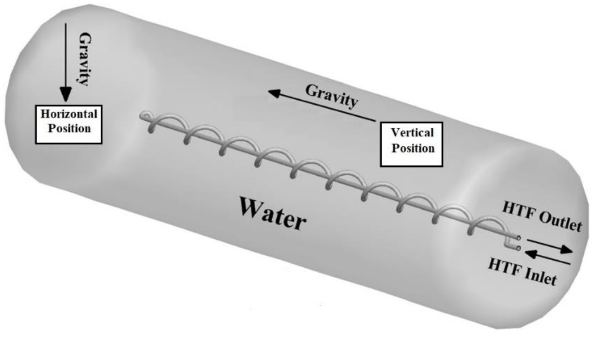
2.1. Geometrical Model

In the present investigation, the ice storage system consists of a cylindrical tank with a volume of 946 L. The considered ice storage system is of shell and tube type (Figure 1), where the length and diameter of the cylindrical shell are 2.5 m and 0.7 m, respectively. The shell is filled with liquid water. Inside the shell, three types of tubes are chosen including a U-shaped tube, a coil tube with an inner return line and a coil tube with an outer return line (see Figure 2). In the following sections, the coil tube with an inner return line and the one with an outer return line are introduced as coil tube-model 1 and coil tube-model 2, respectively. The heat transfer area is constant to ease the direct comparison between the different configurations. The diameters of the U-shaped and coil tubes are 0.026 and 0.018 m, respectively. The pitch of the coil tube is fixed to 0.2 m. The physical properties for pure liquid and solid water are listed in

Table 1. Physical and thermal properties of liquid and solid water [9,24].

Property	Pure Water
	Phase
	Liquid	Solid
Density (ρ) [kg/m3]	999.8	917
Dynamic viscosity (µ) [kg/(m.s)]	0.00162	-
Specific heat (cp) [J/(kg.K)]	4180	2217
Thermal conductivity (k) [W/(m.K)]	0.578	1.918
Heat of fusion (hsf) [J/kg]	334,000
Solidification Temperature [K]	273.15
Thermal expansion coefficient (β) [K−1]	−6.733353 × 10−5	-

, and are supposed to be constant. The fluid flow inside the tube was not considered and instead, a constant temperature boundary condition was assumed for the wall of all the investigated tubes.

2.2. Governing Equations

One solves the 3D conservative equations for mass, momentum and energy in their 3D unsteady formulation. The Boussinesq approximation is used to account for buoyancy effects [25,26]:

$$\rho ={\rho }_0\left(1-\beta \left(\left(T-T_0\right)\right)\right).$$

(1)

The continuity equation writes:

$$\nabla \hspace{0.17em}.\hspace{0.17em}\hspace{0.17em}\overrightarrow{V}=0.$$

(2)

The momentum equation reads:

$$\frac{\partial V}{\partial t}+\overrightarrow{V}.\nabla \overrightarrow{\hspace{0.17em}V}=\frac{1}{\rho }\left(-\nabla P+\mu {\nabla }^2\overrightarrow{\hspace{0.17em}V}+\rho \overrightarrow{g}\beta \left(T-T_{ref}\right)\right)+\overrightarrow{\hspace{0.17em}S}.$$

(3)

The energy equation does not include the viscous dissipation, which is negligible in the present case:

$$\frac{\partial h_{sens}}{\partial t}+\frac{\partial h_{lat}}{\partial t}+\nabla .\left(\overrightarrow{V}{h}_{sens}\right)=\nabla .\left(\frac{k}{\rho c_p}\nabla h_{sens}\right).$$

(4)

The total enthalpy can be obtained by:

$$h_{tot}=h_{sens}+h_{lat},$$

(5)

where:

$$h_{sens}=h_{ref}+\underset{T_{ref}}{\overset{T}{{\displaystyle \int }}}{c}_{p}dT=h_{ref}+c_p\underset{T_{ref}}{\overset{T}{{\displaystyle \int }}}dT,$$

(6)

$$h_{lat}=\mathsf{\lambda } .\mathrm{L}$$

(7)

where h_lat can be in the range of zero and h_sf, for the solid and liquid phases respectively. λ indicates the liquid fraction. L is the latent heat of fusion. The sensible heat can be written as:

$$h_{sens\hspace{0.17em}}=h_{tot}-h_{lat}.$$

(8)

The equation for the liquid fraction writes [27]:

$$\lambda =\left\{\begin{array}{c}\frac{h_{lat}}{h_{sf}}=0\hspace{0.17em}\hspace{0.17em}\hspace{0.17em}if\hspace{0.17em}\hspace{0.17em}\hspace{0.17em}T\le T_s\\ \frac{h_{lat}}{h_{sf}}=1\hspace{0.17em}\hspace{0.17em}\hspace{0.17em}if\hspace{0.17em}\hspace{0.17em}\hspace{0.17em}T\ge T_{liq}\\ \frac{h_{lat}}{h_{sf}}=\frac{T-T_s}{T_{liq}-T_s}\hspace{0.17em}\hspace{0.17em}\hspace{0.17em}if\hspace{0.17em}\hspace{0.17em}\hspace{0.17em}{T}_s<T<T_{liq}\end{array}\right\}.$$

(9)

A temperature difference of 0.1 K is assumed between the liquidus and solidus temperatures. The term S in Equation (3) is the Darcy’s law damping source term, which affects the momentum equation:

$$\overrightarrow{S}=-\frac{{\left(1-\lambda \right)}^2}{{\lambda }^3}{C}_{mush}\overrightarrow{V},$$

(10)

where C_mush is the constant of the mushy zone, which was set to 10⁵ kg/(m³s) [26].

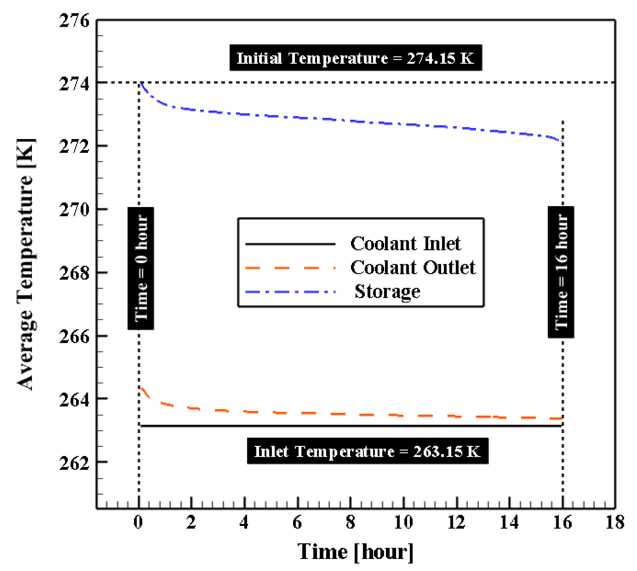
2.3. Initial and Boundary Conditions

The initial temperature of the whole computational domain is fixed to 274.15 K, and all the velocity components are set to zero. The outer walls of the storage tank are considered to be insulated. The fluid flow inside the U-shaped coil tube is not considered and instead, a constant temperature boundary condition is assumed for the wall of the coil tube. So, a fixed temperature of 263.15 K is applied inside the tube walls. In order to explain the reason for relinquishing the coolant fluid in the tube, a comparison between the inlet and outlet temperatures of the coolant fluid at Re = 2000 and T_inlet = 263.15 K is shown in Figure 3. Firstly, the presence of fluid in the coil tube would induce a more refined mesh grid, especially around the tube wall and also inside the tube. Accordingly, a lower time step should be considered which leads to higher computational time. According to Figure 3, when one considers the fluid inside the tube, the difference between the inlet and outlet temperatures of the coolant remains very low (below 1 °C) for about 98% of the simulation time. So, by relinquishing the difference between the inlet and outlet temperatures of the coolant fluid, a constant temperature (−10 °C) can be set at the tube wall.

2.4. Numerical Method

The numerical solver was based on the finite volume method. The governing equations written in a Cartesian frame were solved in 3D in their unsteady formulation through ANSYS Fluent 18.2. The phase change process is simulated by the enthalpy-porosity method described in Section 2.2. The SIMPLE algorithm is used to overcome the velocity-pressure coupling. The spatial discretization for both momentum and energy equations corresponds to the QUICK scheme with a first-order implicit scheme for the temporal discretization. The least-square cell-based is applied for gradient spatial discretization. The continuity, velocity, and energy residuals are set to 10⁻³, 10⁻³, and 10⁻⁶, respectively. Values of under-relaxation factors are fixed to 0.3 for pressure, 1 for density, body forces and energy, 0.7 for the momentum, and finally 0.9 for the liquid fraction update.

3. Results and Discussion

3.1. Model Validation

To validate the flow solver, the present simulations were compared to the experimental data of Sasaguchi et al. [28,29]. They corresponds to the ice formation process around two cylinders with fixed temperatures. Figure 4 displays the temporal evolution of the solid volume ratio, A_S/A_C. This is defined as the ratio of the solidified area to the total cross-sectional area of the cylinders. It can be clearly seen that the numerical results are in fairly good agreement with the experimental results, with a maximum deviation of 8.13% at the maximum flow time.

3.2. Grid and Time-Step Independence Study

A series of tests were done to check the grid independence of the solution for three different mesh grids including 1.3, 1.8 and 2.3 millions of tetrahedral elements. As shown in Figure 5a, the mesh grids with 1.8 and 2.3 million elements provide undistinguishable results. The grid with 1.8 million elements shown in Figure 6 was then selected for all simulations. The grid was refined close to the tube walls, where higher gradients are expected, with a refinement ratio of 1.1. Additionally, some tests were done to evaluate the appropriate time-step. Results obtained with three time-steps, namely 0.5, 1 and 2 s, are compared in Figure 5b. The temporal evolutions of the liquid fraction appear quite similar for the two smaller time-steps. Finally, the time-step is fixed to 1 s in all simulations. The maximum number of iterations per time step was fixed to 100.

3.3. Ice Storage System in the Horizontal Position

In this section, numerical simulations are performed to study the effect of the tube type on the charging process in a horizontal shell. The schematics of the considered models are illustrated in Figure 1 and Figure 2. The temporal evolutions of the liquid fraction (LF) are displayed in Figure 7 for three types of tube for 16 h. Figure 7 shows that using a coil tube, instead of a simple U-shaped tube, leads to higher heat transfer rate between the heat transfer fluid in the tube and water in the shell, denoted as the “produced ice”. Additionally, model 2 with an outer return line exhibited better performance, as compared with model 1 (inner return line). This can be attributed to a higher coverage area in model 2. According to Figure 7, after 8 h of solidification, the case with the coil tube-model 2 has 6% and 8% lower liquid fraction in comparison with the coil tube-model 1 and the U-shaped tube, respectively. After 16 h of solidification, the case with the coil tube-model 2 has 1.057% and 1.32% lower liquid fraction in comparison with the coil tube-model 1 and the U-shaped tube, respectively.

The contours of liquid fraction and temperature at five sections inside the computational domain and at three times including 4, 8 and 12 h are illustrated in Figure 8 and Figure 9, respectively. After 4 h, the differences between the models remain low due to the conduction around the tube, which is the governing heat transfer mechanism. However, as time passes, natural convection affects the heat transfer process, and the differences between the models become more noticeable.

Finally, after 12 h, as shown in Figure 8 and Figure 9, the amount of produced ice in the U-shaped and coil tubes (model 1) is similar. However, the case with the coil tube shows higher produced ice around the coil. The coil tube with an outer return line produces much more ice, as compared with the other models. This can be attributed to the high coverage of the used coil in model 2, which can be clearly seen regarding the temperature contours of Figure 8 and Figure 9. On the other hand, at the coil tube with an outer return line (model 2), the temperature distribution around the coil tube and return line reaches the solidification temperature faster than the other models, and covers more area in the computational domain. The effect of the tube geometry on the ice formation is shown in Figure 10, which displays the contours of liquid fraction for the three models in the horizontal position at time = 5 h and Y = 0. Firstly, using a coil tube, instead of a simple U shaped one, leads to higher produced ice quantity. Secondly, model 2 covers more region, as compared to model 1, which means that model 2 produces more ice than model 1. The effect of the geometry of the return line of the coil tube on the solidification process is shown obviously on the contours of liquid fraction in Figure 10, which confirms the reported results in Figure 8 and Figure 9.

3.4. Ice Storage System in the Vertical Position

In the present section, the tubes are placed in the vertical position. The results in terms of the temporal variations of the liquid fraction (LF) are illustrated in Figure 11 for the three types of tube. The simulations were performed also for 16 h. Figure 11 shows that using a coil tube, instead of a simple U-shaped tube, leads to higher produced ice. Between the studied coil tubes, model 2 with an outer return line exhibits a better performance in comparison with model 1 (with an inner return line), because of the more coverage area in model 2. The results in the vertical position exhibit the same trend as the ones obtained with the horizontal position (Figure 7). The corresponding contours of liquid fraction and velocity magnitude are depicted at midplane Y = 0 in Figure 12 for t = 14 h. Firstly, using a coil tube instead of a simple U-shaped tube leads to higher ice formation. Secondly, a coil tube with an outer return line produces more ice at a fixed time, because of its higher coverage area. The velocity field is set initially at zero. So, according to the contours of the velocity magnitude displayed in Figure 12, it can be seen clearly that the velocity field was not zero for all cases because of the onset of natural convection.

3.5. Comparison between the Horizontal and Vertical Positions

The influence of the ice storage tank position on the ice formation is investigated numerically for the three types of tubes. The temporal variations of the liquid fraction (LF) for three different types of tube including a simple U-shaped tube, a coil tube with an inner return line (model 1), and a coil tube with an outer return line (model 2) are illustrated in Figure 13a–c, respectively, for two different positions of the ice storage tank. Figure 13a shows that for the simple U-shaped tube’s case, until 8 h, there is no noticeable difference between the two positions. However, as time passed, the difference between the models became significant. Finally, after 20 h, this type of ice storage system in its horizontal position produces more ice compared to the tank in the vertical position.

Figure 13b shows that for the case with a coil tube with an inner return line (model 1), before time = 12.6 h, the horizontal position produces more ice than the vertical one. At time = 12.6 h, the amount of produced ice for the two positions are the same. After that, as time passes, the vertical position exhibits better performance in comparison with the horizontal position. It should be noted that the differences between the two positions (for this set of operating conditions and geometrical parameters) remain very small. Contrary to the results obtained in Figure 13b, for the case with a coil tube and an outer return line (model 2), the vertical position shows higher produced ice, as compared with the horizontal one (Figure 13c). The effect of position on the ice formation in the case with a coil tube and an outer return line is significantly more pronounced than the case with a coil tube and an inner return line.

In order to better show the effect of natural convection on the solidification process, the 3D contours of the velocity magnitude for different cases are illustrated in Figure 14 with the system in the vertical position. Natural convection clearly affects the velocity field. However, because the solidification process is here investigated for only 14 h, the ice is formed just around the tube. The simulation time is too short for the liquid fraction to highlight a significant effect of natural convection.

As shown in Figure 13, the position of the storage system (vertical and horizontal) does not affect significantly the ice formation. Natural convection has indeed no noticeable influence on the solidification process, as previously discussed.

To go a little bit further, the three-dimensional streamlines and the contours of the velocity magnitude are illustrated in Figure 15 and Figure 16 for the horizontal and vertical positions, respectively. In the horizontal position (Figure 15), whatever the geometry of the HTF tube, the streamline patterns remain the same. The main vortexes are produced around the Z-axis because of the direction of gravity along the X-axis. In the vertical position (Figure 16), the streamlines get completely different. Streamlines are then a better indicator compared to the average liquid fraction to highlight the influence of natural convection on the solidification process. This is mainly due to the relatively short simulation time (16 h) for such a storage volume and to the external melt type.

4. Conclusions

In the present study, 3D numerical simulations have been carried out to examine the effects of two geometrical parameters, including the tube type and position of the shell, on the solidification process in an ice storage system. Three types of tubes, including a U-shaped tube, a coil tube with an inner return line, and a coil tube with an outer return line as well as two positions of the ice storage tank (horizontal and vertical positions) have been considered. The main result can be summarized as follows:

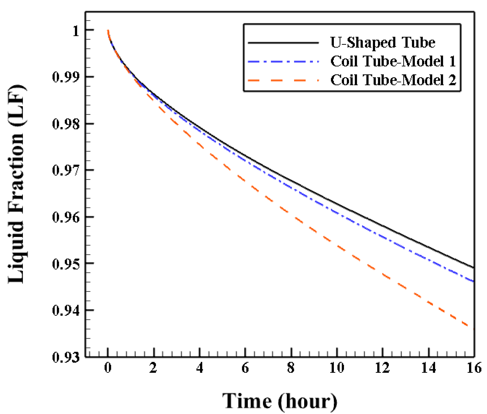
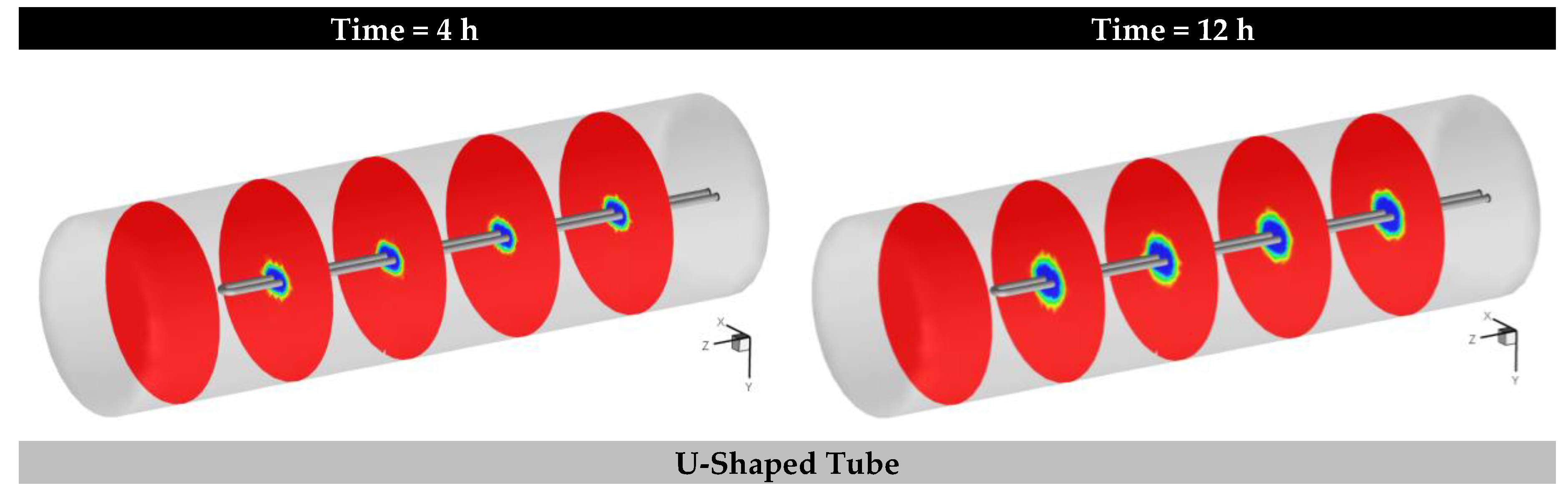
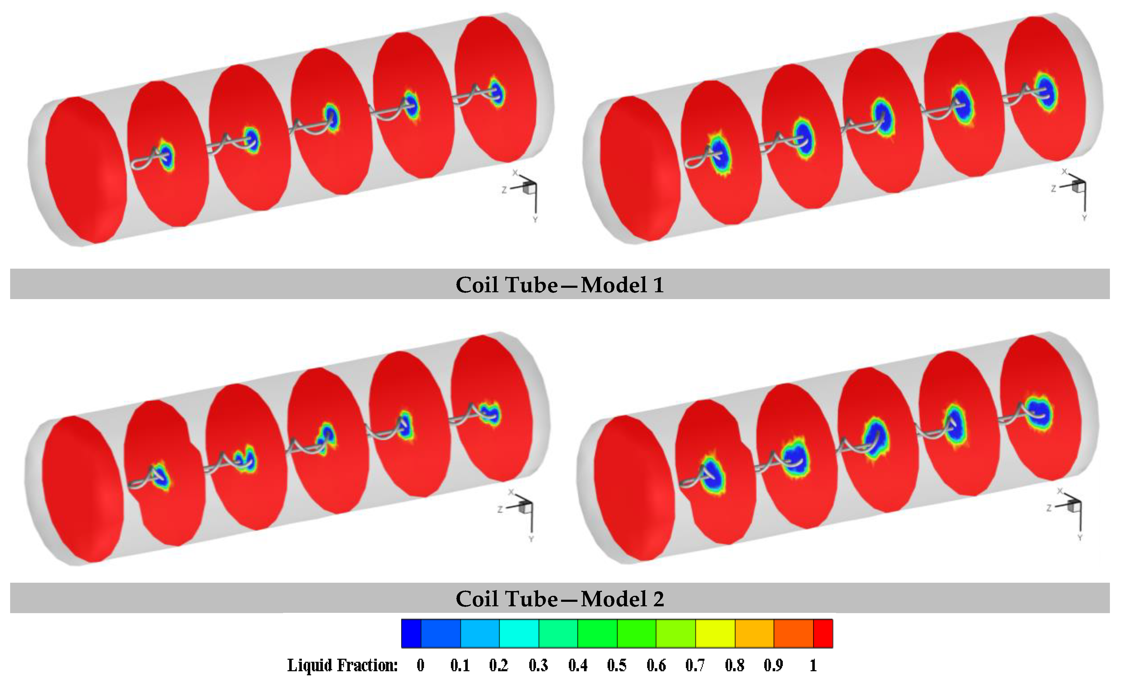
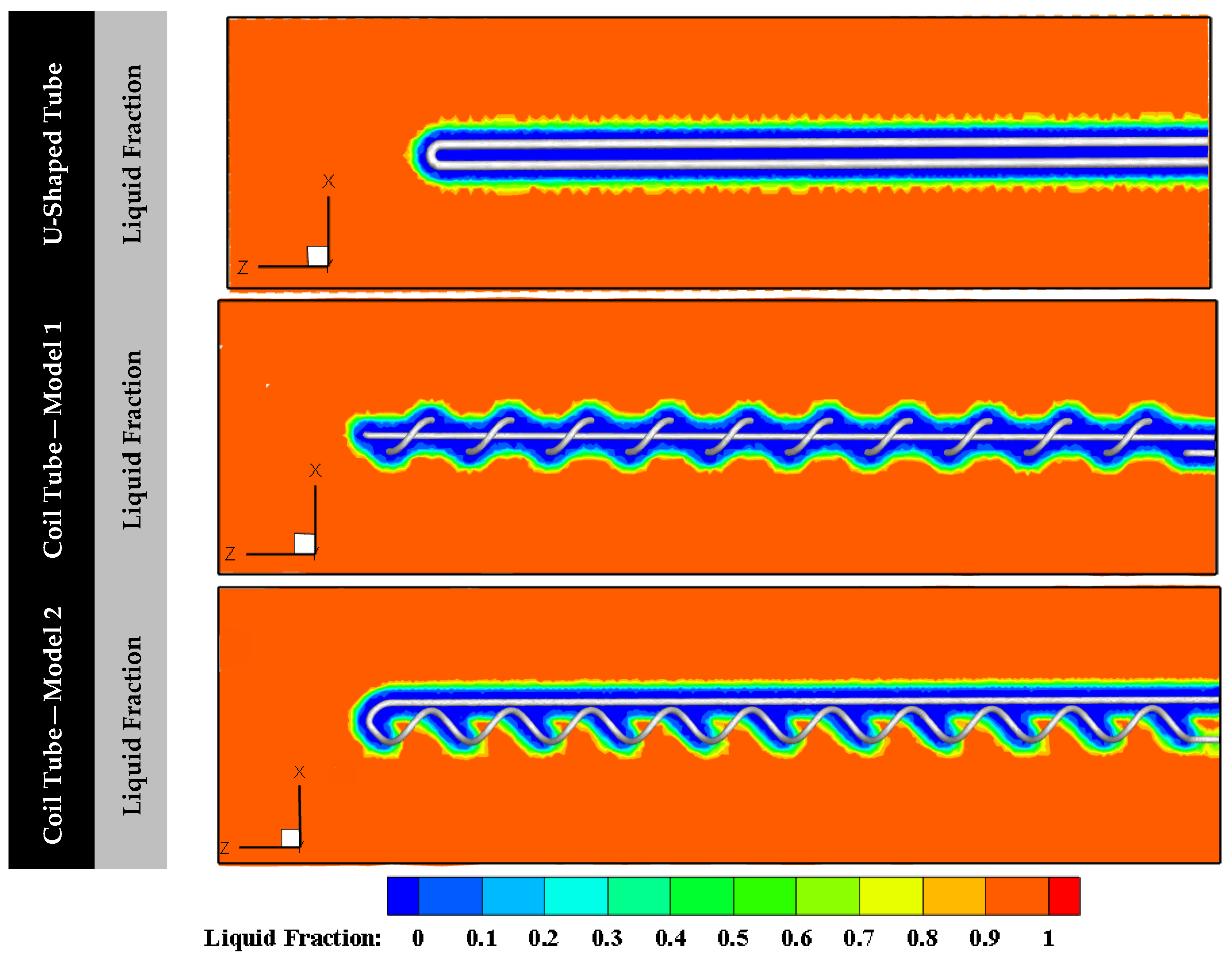
• In both horizontal and vertical positions of the ice storage tank, the coil tube fastens the ice formation, as compared with the simple U-shaped tube. For the cases with the coil tube, the covered area of the domain is higher in comparison with the U-shaped tube, which leads to an increase of the solidification rate.
• Between the different coil tubes, the coil tube with an outer return line exhibits a better performance (more produced ice) compared to the coil tube with an inner return line. In other words, the space through the coil tube solidifies more, even without the return line. The presence of the return line through the coil tube (inner return line) has no significant effect on the solidification rate. However, in the case with the outer return line, the covering area by the HTF tube increases, which leads to a higher solidification rate.
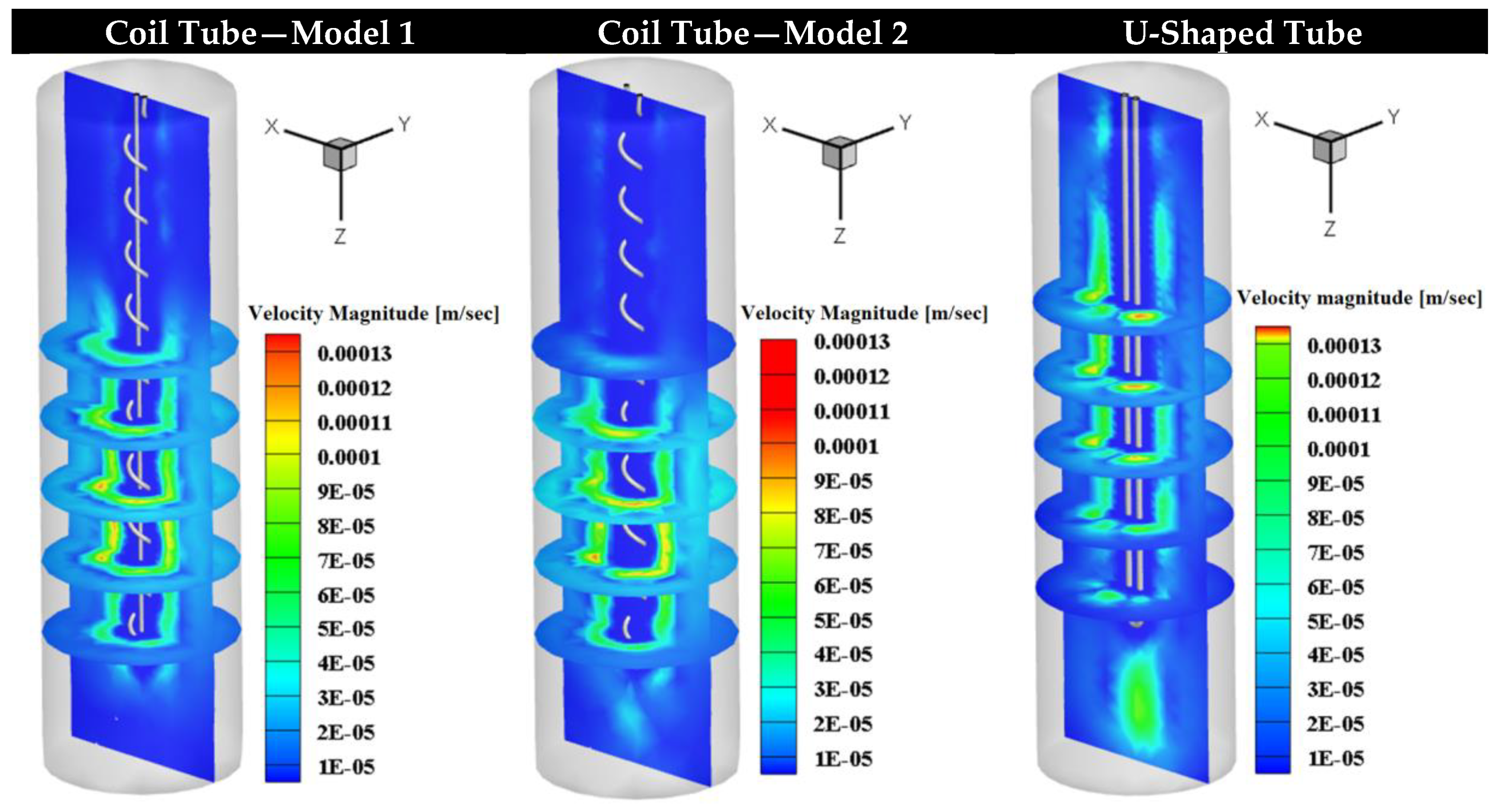
• In the simple U-shaped tube configuration, the horizontal position enhances the ice formation, as compared with the vertical position. For the case with a coil tube and an inner return line, the differences between the two positions for this particular case remain insignificant. The effect of the position on the ice formation for the coil tube with an outer return line is significantly more pronounced than the case with the coil tube and an inner return line. In this case, the vertical position shows higher produced ice than the horizontal position.
• After 8 h of solidification, the coil tube with the outer return line has about 6% and 8% lower liquid fraction in comparison with the coil tube with the inner return line and U-shaped tube, respectively. After 16 h of solidification, the coil tube with the outer return line has about 1.057% and 1.32% lower liquid fraction in comparison with the coil tube with the inner return line and U-shaped tube, respectively for both positions (vertical and horizontal).

It is worth mentioning that, in addition to the present study, a comprehensive study is necessary as future work to study the effect of the coil geometrical parameters on the solidification process in an ice-on-coil ice storage system.

References

1. Pocketbook, S. EU Transport in Figures; Publications Office of the European Union: Luxembourg, 2016.
2. Knebel, D.E. Off-peak cooling with thermal storage. ASHRAE J. 1990, 32, 40–44. [Google Scholar]
3. Basecq, V.; Michaux, G.; Inard, C.; Blondeau, P. Short-term storage systems of thermal energy for buildings: A review. Adv. Build. Energy Res. 2013, 7, 66–119. [Google Scholar] [CrossRef]
4. Thumann, A. Optimizing HVAC Systems; Fairmont Pr: Lilburn, GA, USA, 1988. [Google Scholar]
5. Yi, W.; Dong, W. Modeling and Simulation of Discharging Characteristics of External Melt Ice-on Coil Storage System. Int. J. Smart Home 2015, 9, 179–192. [Google Scholar] [CrossRef] [Green Version]
6. Korti, A.I.N. Numerical Heat Flux Simulations on Double-Pass Solar Collector with PCM Spheres Media. Int. J. Air-Cond. Refrig. 2016, 24, 1650010. [Google Scholar] [CrossRef]
7. Kang, Z.; Wang, R.; Zhou, X.; Feng, G. Research Status of Ice-storage Air-conditioning System. Procedia Eng. 2017, 205, 1741–1747. [Google Scholar] [CrossRef]
8. Rahdar, M.H.; Emamzadeh, A.; Ataei, A. A comparative study on PCM and ice thermal energy storage tank for air-conditioning systems in office buildings. Appl. Therm. Eng. 2016, 96, 391–399. [Google Scholar] [CrossRef]
9. Jannesari, H.; Abdollahi, N. Experimental and numerical study of thin ring and annular fin effects on improving the ice formation in ice-on-coil thermal storage systems. Appl. Energy 2017, 189, 369–384. [Google Scholar] [CrossRef]
10. Shih, Y.-C.; Chou, H. Numerical Study of Solidification around Staggered Cylinders in a Fixed Space. Numer. Heat Transf. Part A Appl. 2005, 48, 239–260. [Google Scholar] [CrossRef]
11. Yang, T.; Sun, Q.; Wennersten, R. The impact of refrigerant inlet temperature on the ice storage process in an ice-on-coil storage plate. Energy Procedia 2018, 145, 82–87. [Google Scholar] [CrossRef]
12. Erek, A.; Ezan, M.A. Experimental and numerical study on charging processes of an ice-on-coil thermal energy storage system. Int. J. Energy Res. 2007, 31, 158–176. [Google Scholar] [CrossRef]
13. Ezan, M.A.; Erek, A.; Dincer, I. Energy and exergy analyses of an ice-on-coil thermal energy storage system. Energy 2011, 36, 6375–6386. [Google Scholar] [CrossRef]
14. Sang, W.H.; Lee, Y.T.; Chung, J.D.; Kim, S.T.; Kim, T.; Oh, C.-H.; Lee, K.-H. Efficient numerical approach for simulating a full scale vertical ice-on-coil type latent thermal storage tank. Int. Commun. Heat Mass Transf. 2016, 78, 29–38. [Google Scholar] [CrossRef]
15. Ajarostaghi, S.S.M.; Poncet, S.; Sedighi, K.; Delavar, M.A. Numerical Modeling of the Melting Process in a Shell and Coil Tube Ice Storage System for Air-Conditioning Application. Appl. Sci. 2019, 9, 2726. [Google Scholar] [CrossRef] [Green Version]
16. Pakzad, K.; Mousavi Ajarostaghi, S.S.; Sedighi, K. Numerical simulation of solidification process in an ice-on-coil ice storage system with serpentine tubes. SN Appl. Sci. 2019, 1, 1258. [Google Scholar] [CrossRef] [Green Version]
17. Afsharpanah, F.; Ajarostaghi, S.S.M.; Sedighi, K. The influence of geometrical parameters on the ice formation enhancement in a shell and double coil ice storage system. SN Appl. Sci. 2019, 1, 1264. [Google Scholar] [CrossRef] [Green Version]
18. Zheng, Z.-H.; Ji, C.; Wang, W.-X. Numerical Simulation of Internal Melt Ice-on-Coil Thermal Storage System. Energy Procedia 2011, 12, 1042–1048. [Google Scholar] [CrossRef] [Green Version]
19. Xie, J.; Yuan, C. Numerical study of thin layer ring on improving the ice formation of building thermal storage system. Appl. Therm. Eng. 2014, 69, 46–54. [Google Scholar] [CrossRef]
20. Xie, J.; Yuan, C. Parametric study of ice thermal storage system with thin layer ring by Taguchi method. Appl. Therm. Eng. 2016, 98, 246–255. [Google Scholar] [CrossRef] [Green Version]
21. Ismail, K.A.R.; Sousa, L.M.; Lino, F.A.M. Solidification of PCM around Curved Tubes Including Natural Convection Effects. Int. J. Energy Eng. 2015, 5, 57–74. [Google Scholar] [CrossRef]
22. Mousavi Ajarostaghi, S.S.; Sedighi, K.; Delavar, M.A.; Poncet, S. Influence of geometrical parameters arrangement on solidification process of ice-on-coil storage system. SN Appl. Sci. 2020, 2, 109. [Google Scholar] [CrossRef] [Green Version]
23. Seddegh, S.; Wang, X.; Henderson, A.D. A comparative study of thermal behaviour of a horizontal and vertical shell-and-tube energy storage using phase change materials. Appl. Therm. Eng. 2016, 93, 348–358. [Google Scholar] [CrossRef]
24. Michalek, T.; Kowalewski, T.; Sarler, B. Natural convection for anomalous density variation of water: Numerical benchmark. Prog. Comput. Fluid Dyn. Int. J. 2005, 5, 158. [Google Scholar] [CrossRef] [Green Version]
25. Brent, A.; Voller, V.; Reid, K. Enthalpy-porosity technique for modeling convection-diffusion phase change: Application to the melting of a pure metal. Numer. Heat Transf. Part A Appl. 1988, 13, 297–318. [Google Scholar]
26. Faghri, A.; Zhang, Y. Transport Phenomena in Multiphase Systems; Elsevier: Amsterdam, The Netherlands, 2006. [Google Scholar]
27. Voller, V.; Prakash, C. A fixed grid numerical modelling methodology for convection-diffusion mushy region phase-change problems. Int. J. Heat Mass Transf. 1987, 30, 1709–1719. [Google Scholar] [CrossRef]
28. Sasaguchi, K.; Kusano, K.; Viskanta, R. A numerical analysis of solid-liquid phase change heat transfer around a single and two horizontal, vertically spaced cylinders in a rectangular cavity. Int. J. Heat Mass Transf. 1997, 40, 1343–1354. [Google Scholar] [CrossRef]
29. Sasaguchi, K.; Kusano, K.; Kitagawa, H. Solid/Liquid Phase Change Heat Transfer around Two Horizontal, Vertically Spaced Cylinders. An Experimental Study on the Effect of Density Inversion of Water. Trans. Jpn. Soc. Mech. Eng. Ser. B 1995, 61, 208–214. [Google Scholar] [CrossRef] [Green Version]
Figure 1. Schematic view of the computational domain presenting the two considered positions, horizontal and vertical.
Applsci 10 01059 g001
Figure 2. Three types of tubes considered in the present paper: (a) U-shaped tube, (b) coil tube model 1, and (c) coil tube model 2.
Applsci 10 01059 g002
Figure 3. Comparison between the inlet and outlet temperatures of the coolant fluid at Re = 2000 and Tinlet = 263.15 K.
Applsci 10 01059 g003
Figure 4. Comparison between the present simulations and the experimental results of Sasaguchi et al. [27,28]. The solid volume ratio (AS/AC) is the ratio of the solidified area to the total cross-sectional area of the cylinders.
Applsci 10 01059 g004
Figure 5. Grid (a) and Time-step (b) independence tests.
Applsci 10 01059 g005
Figure 6. Example of the mesh grid used for the (a) coil tube and (b) shell.
Applsci 10 01059 g006
Figure 7. Temporal evolution of the liquid fraction for three types of tubes in the ice on the coil ice storage system in the horizontal position.
Applsci 10 01059 g007
Figure 8. Contours of the liquid fraction (LF) at five various sections of the shell for the three types of tubes and the system in the horizontal position.
Applsci 10 01059 g008aApplsci 10 01059 g008b
Figure 9. Contours of temperature (K) at five various slices in the computational domain for the different investigated models in the horizontal position.
Applsci 10 01059 g009aApplsci 10 01059 g009b
Figure 10. Contours of liquid fraction and temperature (K) for three types of tube in the horizontal position after 5 h and at midplane Y = 0.
Applsci 10 01059 g010
Figure 11. Temporal evolution of the liquid fraction for three types of tubes in the ice on coil ice storage system in the vertical position.
Applsci 10 01059 g011
Figure 12. Contours of liquid fraction and velocity magnitude (m/s) for three types of tube in the vertical position after 14 h and at midplane Y = 0.
Applsci 10 01059 g012
Figure 13. Comparison between two positions of the ice-on-coil ice storage system: (a) single U-shaped, (b) coil tube-model 1, (c) coil tube-model 2.
Applsci 10 01059 g013
Figure 14. Three-dimensional contours of the velocity magnitude (m/s) for the three models.
Applsci 10 01059 g014
Figure 15. Three-dimensional streamlines with contours of the velocity magnitude for the three different cases in the horizontal position.
Applsci 10 01059 g015aApplsci 10 01059 g015b
Figure 16. Three-dimensional streamlines with contours of the velocity magnitude for the three different cases in the vertical position.
Applsci 10 01059 g016