Contextual Coefficients Excitation Feature: Focal Visual Representation for Relationship Detection

Abstract

Visual relationship detection (VRD), a challenging task in the image understanding, suffers from vague connection between relationship patterns and visual appearance. This issue is caused by the high diversity of relationship-independent visual appearance, where inexplicit and redundant cues may not contribute to the relationship detection, even confuse the detector. Previous relationship detection models have shown remarkable progress in leveraging external textual information or scene-level interaction to complement relationship detection cues. In this work, we propose Contextual Coefficients Excitation Feature (CCEF), a focal visual representation, which is adaptively recalibrated from original visual feature responses by explicitly modeling the interdependencies between features and their contextual coefficients. Specifically, contextual coefficients are obtained by calculation of both the spatial coefficients and generated-label ones. In addition, a conditional Wasserstein Generative Adversarial Network (WGAN) regularized with a relationship classification loss is designed to alleviate inadequate training of generated-label coefficients due to long tail distribution of relationship. Experimental results demonstrate the effective improvements of our method on relationship detection. In particular, our method improves the recall from 8.5% to 23.2% of predicting unseen relationship from zero-shot set.

1. Introduction

With rapid development of deep learning and image recognition [1,2,3,4,5], visual relationship detection [6], a higher-level visual understanding task, has been a popular research topic. Relationships are commonly defined as triplets consisting of a subject, predicate and object, which can be represented as 〈subject, predicate, object〉. Subject and object are considered as the context of predicate [7]. Visual relationship detection aims to recognize various visually observable predicates between subject and object, where subject and object are a pair of objects in the image.

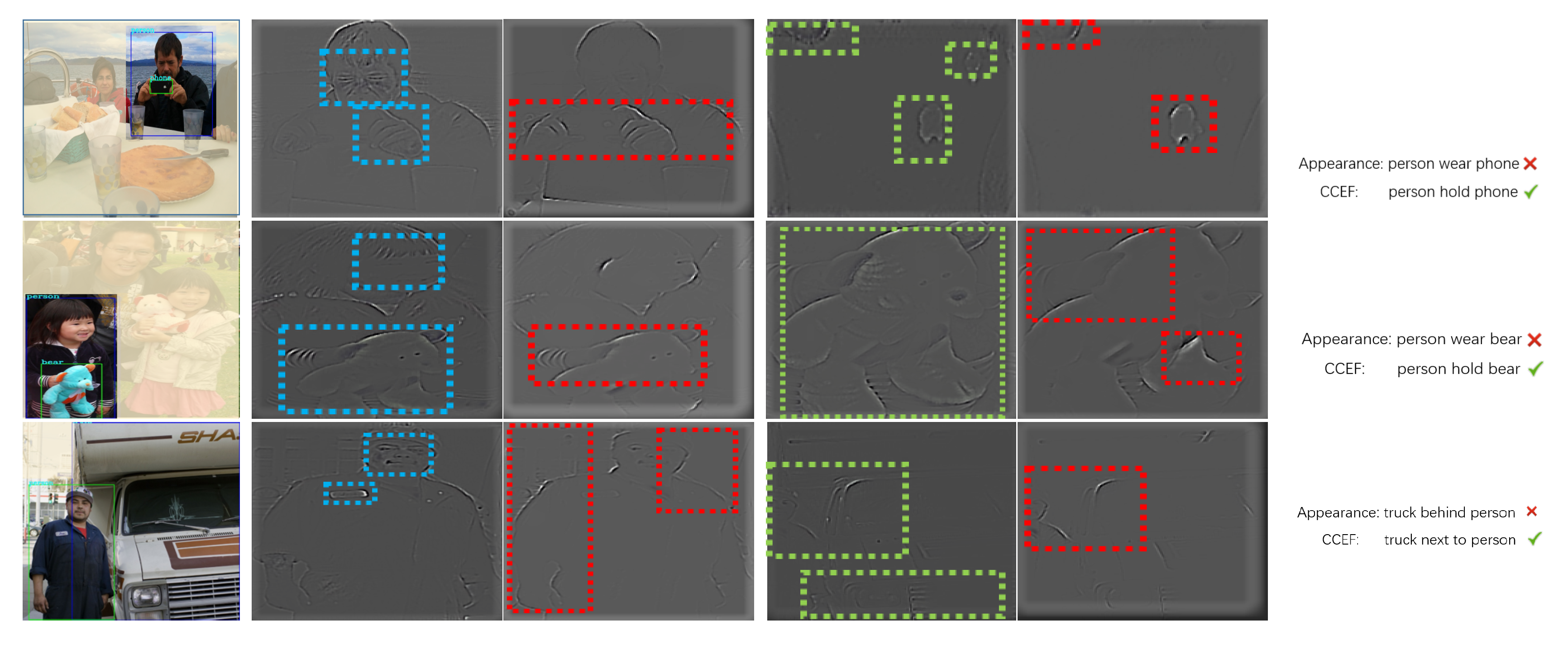
However, visual relationship detection is a challenging task that most existing relationship detection methods [8,9] treat each type of relationship predicates as a class, leading to the high diversity of visual appearance which varies greatly with different relationship instances. Furthermore, this visual diversity undermines the correlation between relationship predicates and visual appearance and confuses the detector. For instance, as Figure 1 shows, when we recognize the predicate “hold” from “people hold phone” and “person hold bear”, person features close to the “phone” or “bear” are more pivotal than other redundant visual features, such as various facial features of different instances. These unrelated features account for the majority of the original visual features and cause the vague connection between visual cues and relationship predicates.

Previous methods [8,10] adopt a linguistic model conditioned on the label of object pairs and predicates, or establish a scene graph relying on the contextual objects in the image to complement insufficient correlations between visual cues and relationship predicate. However, these methods ignore the importance of selectively highlighting the visual features associated with the relationship.

To this end, we propose a novel Contextual Coefficients Excitation Feature (CCEF), which is a focal representation based on a new relationship space. A relation is a predicate. By learning the context of the predicate, that is, the feature distribution of both subject and object in the new space, the noises in their raw visual features are restrained, so their more discriminative representations for relationship predicates are activated. In particular, the contextual coefficients are used to control the importance of both subject and object to predicate, which are learned from both spatial and semantic information. And semantic information is generated by a conditional WGAN [11] regularized by a relationship classification loss. This additional classification loss enforces the generation model to generate relationship-relevant coefficients which are more suitable for relationship detection, especially for predicates with unseen or few training instances. After the contextual coefficients are obtained, both subject and object will be recalibrated on the feature level so as to activate the visual feature that are helpful for predicate selection, that is the CCEF.

Therefore, the visualization of relationship feature in both subject and object is given by deconvolusion approach [12], as shown in Figure 1,to illustrate that CCEF is more significant for relationship representation than original visual features. We summary our contributions as follows:

• Propose a Contextual Coefficients Excitation Feature (CCEF), which reduce the diversity of unrelated visual features by introducing feature recalibration conditioned on the relationship contextual information.
• Improve the conditional WGAN with relationship classification loss for generated-label coefficients generation on VRD and significantly improve the prediction for unseen relationship.

2. Related Works

In this secion, the existing works related to our proposal are briefly reviewed. It is mainly divided into two parts: Visual Relationship Detection and Generative Adversarial Network.

2.1. Visual Relationship Detection

The relationship models are commonly divided into two categories: the joint models [13] and the separate ones [7,8,9]. Early works [14] focused on the joint models and hand-crafted features were used in detection task, which concerned about how to classify the relationship combinations. Since there are too many combinations and the long-tail distribution of visual relationship in the real world, it is impossible to obtain sufficient training images of per combination. As a result, these methods have poor generalization ability.

Therefore, Lu [8] proposed the separate model, formalized the visual relationship detection as a task and provided a new dataset Visual Relationship Detection (VRD). After that, the separate models became the mainstream of research. Despite the visual features and language priors in [8], Zhu [15] complemented the spatial feature of relationship, which was ignored by LP [8]. Zhang [16] introduced the Knowledge Transfer to interpret the relationship as a vector translation, which was trained in an end-to-end system.

Besides, recent works focus on the object priors or textual priors. Zhuang [7] obtained a part of the classifier weight from the context information of relationship and focused on the different image regions via the attention mechanism. Yu [9] utilized massive external textual data and integrated the probability deviation of object pairs into relationship classification. To fully exploit the potential of feature learning, Yin [17] proposed the message passing to encourage the feature sharing between objects and predicate. Moreover, the latest approaches [10,18,19] tried to introduce information of scene graph and tackled the insufficient visual cues and tackled the quadratic combinations of possible relationships.

2.2. Generative Adversarial Network

The main idea of Generative Adversarial Network (GAN) [11,20,21,22,23] is to train a generator that can capture the real data distribution and a discriminate network that discriminates whether an instance is from the truth data distribution or candidates produced by the generator.

The most critical issue of GAN is the convergence of the training. Many works [11,21] have been proposed to address this problem by improving the objective functions of GANs. Arjovsky [11] extended the objective of the original GAN [20] which is related to Jenson-Shannon distance by analyzing the properties of four different divergences or distances over two distributions and proposed WGAN which used the Wasserstein distance to stably optimize discriminators and generators. However, there are also the vanishing and exploding gradient problems in WGAN due to the weight clipping [11]. Thus, Gulrajani [21] improved the WGAN with the gradient penalty. Besides, the input to a generator is a “noise” vector z drawn from a latent distribution, such as a multivariate Gaussian, leading to the uncontrolled generated result. In order to direct the generation process with additional information, Mirza [24] proposed the conditional GAN, which could generate the input-related results by inputting specified labels or attributes into both discriminator and generator.

Despite the generation stability of GANs has been significantly enhanced, improving the quality of generated images is still a challenge. Some other works [25,26,27,28,29,30] focused on deepening the network structure or increasing the training scale have been proposed to improve the quality of images for GANs. In addition to generating realistic images, GANs have shown remarkable results in generating image features [31,32,33]. Xian [33] proposed f-CLSWGAN to tackle generalized zero-shot learning by generating Convolutional Neural Network (CNN) features for unseen classes, which focused on the image features for classification instead of realistic images.

3. Methods

We begin by defining the problem of our interest. Let $O=\left\{(M_i,V_i,y_i,C\left(y_i\right),B_i)\right\}$ where O is the set of localized objects in the image, the subscript i stands for the localized object with index i in object set O. $V_i\in {\mathbb{R}}^{d_V}$ is the visual feature and $M_i\in {\mathbb{R}}^{d_M}$ is contextual coefficient of $V_i$, where $d_M$ and $d_V$ are equivalent. $y_i$ is the object label, $C\left(y_i\right)\in {\mathbb{R}}^{d_c}$ is the word vector [34] of $y_i$ and $B_i=(x_i,y_i,w_i,h_i)\in {\mathbb{R}}^4$ is bounding boxes.

3.1. CCEF: Focal Visual Representation

First, ours proposed $R_i$ is the focal visual representation, which adaptively focus on the local dimensions of each object viusal features for relationships. It is constrained by the label and spatial information to boost the discriminability of representation. $R_i$ is defined as follows:

$$R_i=\mathbf{F}(M_i,V_i),$$

(1)

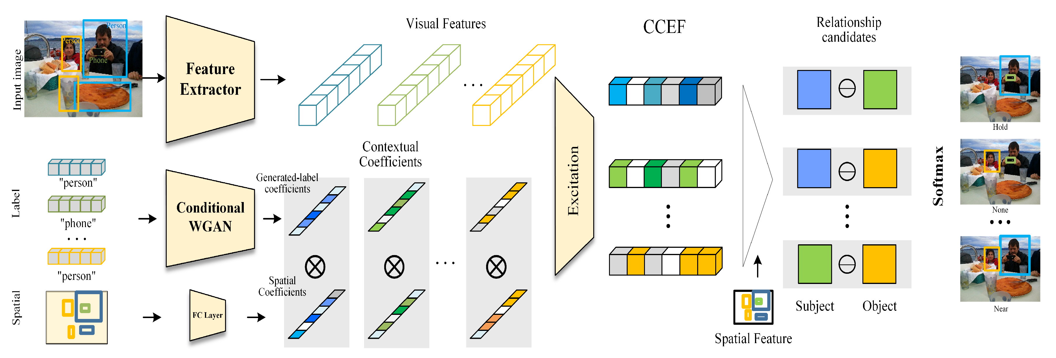
where $\mathbf{F}(·)$ refers to the feature-wise excitation and original visual features $V_i$ are obtained by feeding image regions of object to the feature extractor [2], as in Figure 2.

Contextual Coefficients. The contextual coefficient $M_i$ indicates the importance of each object visual features which is based on label and spatial descriptors, designed as:

$$M_i=G_i\otimes F_i,$$

(2)

where $G_i$ is the generated-label coefficient from the object label with the conditional WGAN and $F_i$ is the spatial coefficient. ⊗ denots the elements-wise multiplication to ensure that multiple dimensions are allowed to be emphasised opposed to one-hot activation. so as in Figure 2.

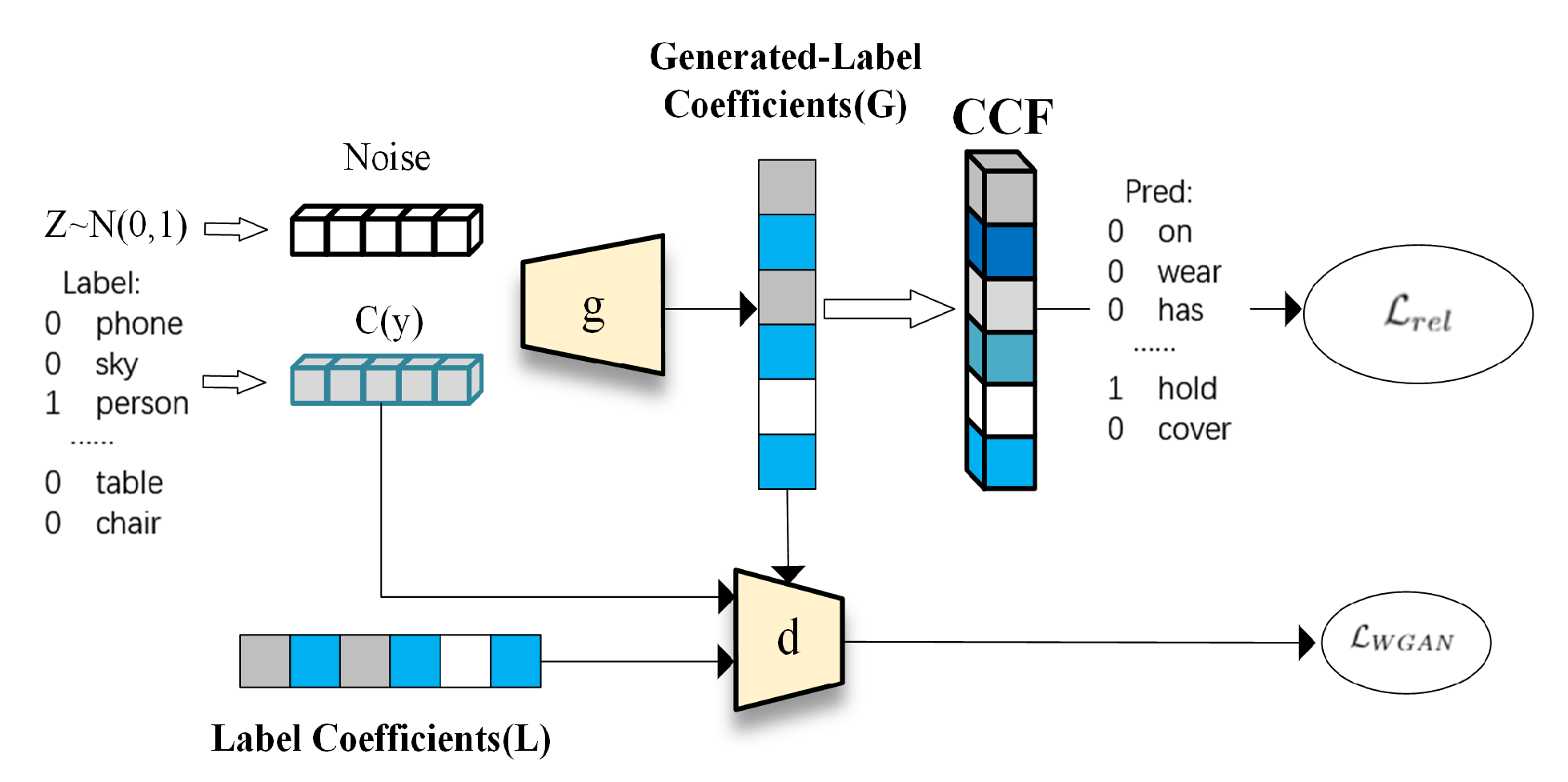
Generated-label coefficients. The generated-label coefficient $G_i$, as a part of importance descriptor, is relationship-related semantics. It is mapped from pure semantic feature space to relationship-related space by conditional WGAN and defined as:

$$G_i=g(z_i,C\left(y_i\right)),$$

(3)

where function g (parameterized by ${\theta }_g$) is the generator of conditional WGAN, $z_i\in {\mathbb{R}}^{d_z}$ is a random noise vector sampled from a multidimensional centered Gaussian and $C\left(y_i\right)$ is the condition vector to direct the coefficients generation process. Besides, the discriminator d (parameterized by ${\theta }_d$) tries to distinguish whether generated-label coefficient can represent label coefficient with the conditional vector $C\left(y_i\right)$ or not. The components d and g iteratively play the two-player minimax game with the objective function, where d tries to maximize the GAN loss and g tries to minimizes it. The structure of our conditional WGAN is shown in Figure 3.

Spatial coefficients. The spatial coefficient $F_i$ is the embedding of object spatial information, defined as follows:

$$F_i=r\left(S_i\right|{\theta }_s),$$

(4)

where $r(·)$ is the Fully Connected layers (FC) layer with ReLU activation, ${\theta }_s$ is the parameter of FC layer. Specifically, $S_i$ is the spatial feature from the bounding boxes of object pairs, similar to the ones in [16]:

$$\left[\frac{x_i-x_j}{w_j},\frac{y_i-y_j}{h_j},log\frac{w_i}{w_j},log\frac{h_i}{h_j}\right],$$

(5)

where $(x_i,y_i,w_i,h_i)$ and $(x_j,y_j,w_j,h_j)$ are bounding boxes of candidated object pairs $B_i$ and $B_j$. Note that subscript i, j indicate different object instances.

Relationship Representation. Referring to the TransE [16,35], the relationship representation $R_{rel}$ is modeled as the translation vector of object reprensatation pairs($R_i$ and $R_j$) by mapping them to the relation space. It is defined as follows:

$$R_{rel}=R_i\ominus R_j,$$

(6)

where ⊖ denotes element-wise subtraction, so as in Figure 2.

Although focal visual representation encodes the appearance of both objects, it is difficult to directly model spatial correlation between predicates and objects with pixel values of image. Hence, final prediction of the relationship is obtained by a line classifier conditioned on the concatenation of S and $R_{rel}$, as:

$$\begin{array}{cc}\hfill P_{rel}=& softmax\left(pre\right|(R_{rel}\circ S);{\theta }_p)\hfill \\ \hfill =& \frac{exp\left({\left({\theta }_p\left(pre\right)\right)}^T(R_{rel}\circ S)\right)}{{\sum }_{c}exp\left({\left({\theta }_p\left(c\right)\right)}^T(R_{rel}\circ S)\right)},\hfill \end{array}$$

(7)

where ${\theta }_p$ is the parameter of the classifier, ∘ denotes vector concatenation.

3.2. Objective Function

Relationship Classification Loss. The visual relationship prediction is constrained by efficient softmax that only rewards the deterministically accurate predicates:

$${\mathcal{L}}_{rel}\left({\theta }_p\right)=-\mathbb{E}\left[log\left(P_{rel}\right)\right].$$

(8)

GAN Loss. As described above, the WGAN-GP [21], which constrains the inactivated truth value in the objective function and enhances the Lipschitz constraint by gradient penalty, is extended to the conditional GAN by integrating a conditional vector into both the generator and discriminator. Besides, the regularization with the relationship classification loss is minimized to encourage the generator to construct suitable label coefficients for relationship detection. Hence, the conditional WGAN is trained with the following objective function:

$${\theta }_g^{*},{\theta }_d^{*}=arg\underset{d}{min}\underset{g}{max}{\mathcal{L}}_{WGAN}+\alpha {\mathcal{L}}_{rel}({\theta }_p^{*},{\theta }_g),$$

(9)

where $\alpha$ in (9) is the balance hyper-parameter to weight the contribution of the classifier loss and the adversarial loss ${\mathcal{L}}_{WGAN}$ is as follows:

$$\begin{array}{cc}\hfill {\mathcal{L}}_{WGAN}=& \mathbb{E}\left[d\right(L,C\left(y\right)\left)\right]-\mathbb{E}\left[d\right(G,C\left(y\right)]\hfill \\ \hfill -& \lambda \mathbb{E}\left[\right(\parallel {\nabla }_{\widehat{L}}{d(L,C\left(y\right))\parallel }_2-1{)}^2],\hfill \end{array}$$

(10)

where $\mathbb{E}[·]$ is the expected value operator, L is the target label coefficient, $\widehat{L}=bL+(1-b)G$ with $b\sim U(0,1)$ and $\lambda$ is a penalty parameter. The first two terms in (10) represent the Wasserstein distance and the third term enforces the gradient of $d(·)$ to satisfy the Lipschitz constraint.

3.3. Training and Prediction

In practice, we design a two-step procedure for our proposed method. During the first stage, the model, shown in Figure 2, is trained by replacing the Conditional WGAN with a FC layer to obtain a pre-trained parameter ${\theta }_p^{*}$. Besides, $G_i$ in (2) are replaced with $L_i$ which are obtained from the labels embeddig of object $C\left(y_i\right)$ with the FC layers similar as (4). In addition, $L_i$ is called label coefficient, which is the necessary target of generated-label coefficients for the training of discriminator because of the unique training mechanism.

After that, in the second stage, the Conditional WGAN which is removed in the first stage is recovered and trained with parameter ${\theta }_p^{*}$. With the trained label coefficients L in the first stage, the discriminator tries to distinguish the generated-label coefficients G from the trained one L. Then the ${\theta }_g,{\theta }_d$ are obtained by training the objectives function as in (9).

Finally, the relationship predication result formulated:

$$re{l}^{*}=arg\underset{pre}{max}softmax\left(pre\right|(R_{rel}\circ S);{\theta }_p^{*}),$$

(11)

where ${\theta }_p^{*}$ is pre-trained in the first step and frozen during training the conditional WGAN.

4. Results

To demonstrate the effectiveness of our proposed visual representation, a series of ablation experiments of our proposed visual representation are compared with existing baseline methods. The experimental setup is as follows:

• Appearance: Directly use $V_i$ to instead $R_i$ in (1) without utilizing any coefficients.
• Outs − A + S: Replace $M_i$ with $S_i$ in (1) in Section 3.1.
• Ours − A + L: Replace $M_i$ with $L_i$ in (1) described as Section 3.2.
• Ours − A + S + L: Replace the $G_i$ with $L_i$ in (2) described in Section 3.2.
• CCEF(Ours − A + S + G): Use visual representation described as Section 3.1.

Here, A is for appearance, S for spatial representation, L for label representation and G for generated-label representation.

4.1. Implement Details

The discriminator consists of two MultiLayer Perceptron (MLP) layers with LeakyReLU activation, while the generator contains one MLP layer with LeakyReLU and an output layer with ReLu. Adam [36], an algorithm for first-order gradient-based optimization of stochastic objective functions and based on adaptive estimates of lower-order moments, is perfect for optimizing the classifier. And Stochastic gradient descent (SGD) is commonly used to optimize both generator and discriminator networks where the learning rate is 0.0001. The balance term $\alpha$ in the loss function is 1.0 coming from experiments, and $\lambda$ = 10 as suggested in [21]. The noise z is drawn from a unit Gaussian with the same dimension as label embedding. The VGG-16 [2] network pre-trained on ImageNet [5] is always used to extract the original visual features. The parameter size of our method is about $135M$ and there is about $15.47\times {10}^9$ floating point operations (FLOPs) in our method.

4.2. Evaluation on Visual Relationship Dataset

Visual Relationship Detection (VRD) dataset [8] is used to evaluate the proposed methods. This dataset contains 5000 images with 100 object categories and 70 predicate categories. In total, there are 37,993 relationship instances with 6672 relationship types and 24.25 predicates per object label. The train/test split is the same as [8], where 4000 training images containing 30,355 relationships with 6672 types and 1000 test images containing 7638 relationships with 2747 types. Note that 1169 relationships with 1029 types are only in the test data.

Our approach are evaluated on three tasks [8]: Predicate detection: with an image and a set of ground truth object bounding boxes, this task is to predict a set of possible predicates between pairs of objects. Since relationship between the pair of objects is critical, this indicator can reflect the performance of the model intuitively, ignoring the error of object detection. Phrase detection: given an input image, this task is to output the triplets 〈subject, predicate, object〉 and localize the entire relationships as one bounding box. Relationship detection: with an input image, it should output the triplets 〈subject, predicate, object〉 and localize the subject and object bounding boxes. Both phrase and relationship bounding boxes should have at least 0.5 overlap with their ground truth bounding boxes. Obviously, the performance of phrase and relationship detection is affected by the result of object detection due to the pipeline of separate detection. In order to compare the performance of relationship models fairly, the object detection results (both bounding boxes and corresponding detection scores) provided by [8] are used for Phrase detection and Relationshop detection. More details in [8].

Following the original paper [8], the Recall@50 (R@50) and Recall@100 (R@100) are used as our evaluation metrics. Recall@X computes the rate of the correct relationship on the top X prediction. The reason of using Recall@x instead of the mean average precision (mAP) is that mAP would penalize the correct detection if dataset don’t have particular ground truth. Note that only the predicate with highest confidence for each pair of objects is considered for predicate, where the prediction score is the product of predicate score and the confidence scores of both subject and object for phrase detection or relationship detection, while prediction score is the predicate score for predicate detection task.

5. Comparison and Discussion

Predicate Detection. The results of predicate detection are reported in

Table 1. Evaluation of different methods on VRD including the R@100/50 of predicate detection on entire and zero-shot set. “*” marks the results of LK without knowledge distillation. And “–” indicates “not applicable”.

Method	Entire Set	Zero-Shot
	R@100/50 ${}^1$	R@100/50
Language Priors [8]	47.9	8.5
VTransE [16]	44.8	–
STA [37]	48.0	20.6
VSA-Net [38]	49.2	–
Zoom-Net [17]	50.7	–
LK [9] *	47.5	17.0
Visual Spatial [15]	51.5	14.6
TFR [39]	52.3	17.3
SA-Full [40]	52.6	21.6
CAI [7]	53.6	16.4
Appearance	45.2	13.2
Ours − A + S	48.5	20.4
Ours − A + L	50.5	15.4
Ours − A + S + L	53.0	19.5
CCEF (Ours − A + S + G)	55.5	23.2

${}^1$ In predicate detection, R@100 and R@50 are equivalent (also observed in [8,9]) because there are not enough located objects in ground truth to produce over 50 pairs.

. The benefit of visual feature excitation is visible across all experiment settings: all kind of coefficients are effective while CCEF achieves better performance. (e.g., R@50 is improved from 45.2% to 55.5% on the entire set and from 13.2% to 23.2% on the zero-shot set).

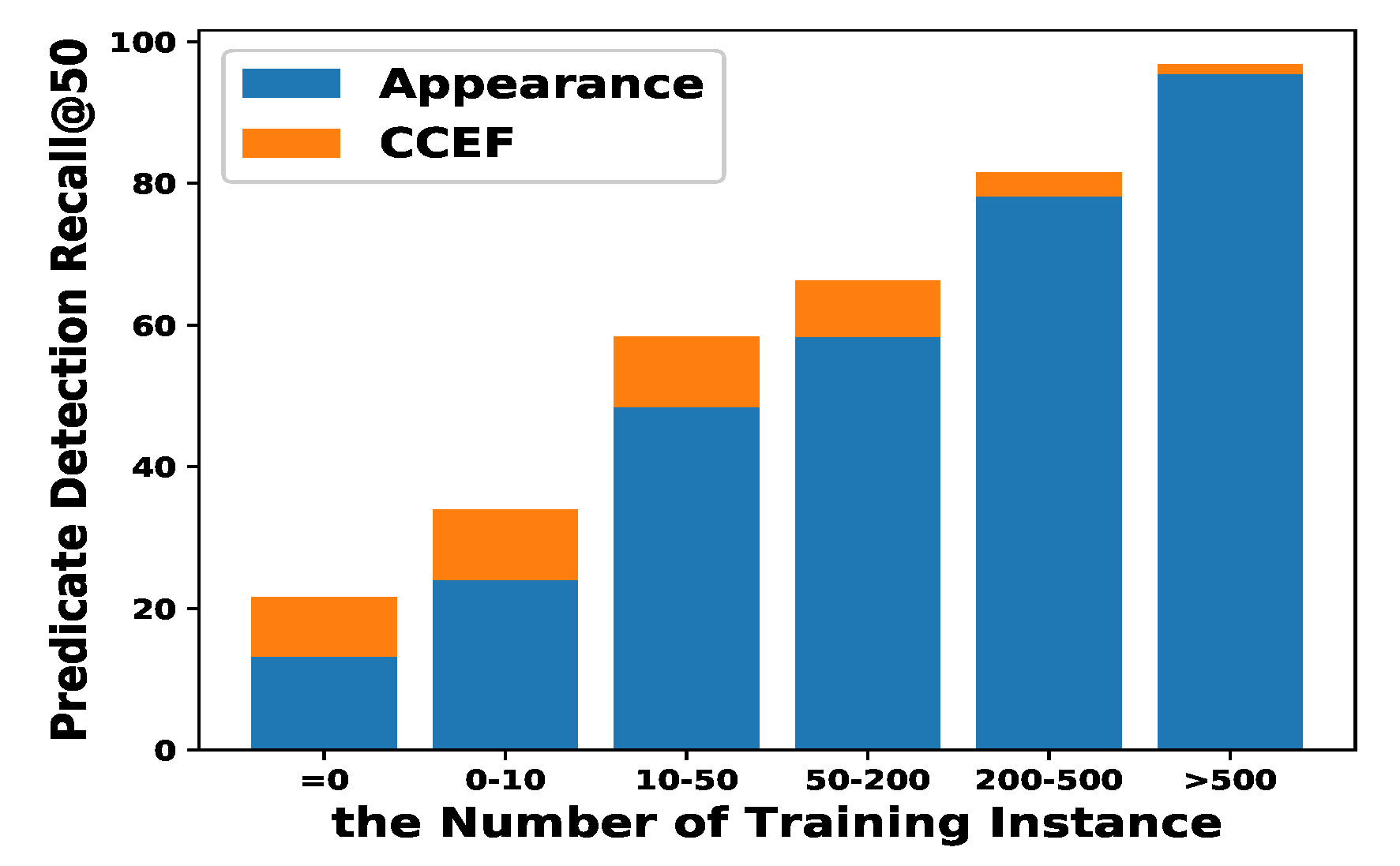
In Table 1, (Appearance) only uses visual information and gets unsatisfactory performance. Then the spatial information is added in (Ours − A + S), which can enhance local visual feature where objects are more likely to interact, and improves the performance of 3 points. Next, the label semantic information is introduced in (Ours − A + L), instead of the spatial information. It reweights the identity information corresponding to the object category in the visual features, which significantly improves the performance of 5 points. Now we can see the performance of (Ours − A + L + S) is 53.0 ($\approx 45.2+3+5$), which proves that label and spatial information can effectively complementary. In the end, CCEF (Ours − A + S + G) replaces the label coefficient (L) in (Ours − A + L + S) with the generated-label coefficient (G) synthesized by the conditional WGAN. We can see the total performance of CCEF (Ours − A + S + G) improves by from 53.0 to 55.5, as shown in Figure 4, which proves that the generated-label coefficient G can effectively improve model generalization and the prediction ability of the unseen relationship, thus improves the overall performance. The G effectively improve model generalization and the prediction ability of the unseen relationship, as shown in Figure 4. Hence, the total performance of CCEF (Ours − A + S + G) improves by from 52.3 to 55.5.

Another interesting finding is that the (Ours − A + S) shows significant improvement on zero-shot. We speculate the reason is that spatial coefficients come from the spatial features which are triplet-independent and are less susceptible to the long tail distribution of training data.

Phrase and Relationship Detection. To fairly compare the performance of relationship models, the same object detection results [8,15] are utilized. Relationship for every pair of object is predicted with the pipeline in Figure 2. Evaluation results on the entire test set and the zero-shot setting are shown in

Table 2. Results of phrase detection and relationship detection on VRD and Zero-Shot Set (ZS).

	Entire Set				Zero-Shot
Method	Phrase Det		Relationship Det		Phrase Det		Relationship Det
	R@100	R@50	R@100	R@50	R@100	R@50	R@100	R@50
Language Priors [8]	17.0	16.2	14.7	13.9	3.8	3.4	3.5	3.1
Visual Spatial [15]	18.9	16.9	15.8	14.3	3.5	3.2	3.0	2.9
TFR [39]	19.1	17.4	16.8	15.2	7.1	5.8	6.5	5.3
CAI [7]	19.2	17.6	17.4	15.6	6.6	6.0	6.0	5.5
SA-Full [40]	19.5	17.9	17.1	15.8	7.8	6.8	7.4	6.4
Appearance	16.9	15.4	14.8	13.5	5.9	5.3	5.5	5.0
Ours − A + S	18.2	16.3	15.9	14.2	8.4	7.1	7.6	6.5
Ours − A + L	19.4	17.8	16.9	15.6	6.2	5.9	5.6	5.2
Ours − A + S + L	19.8	17.3	17.2	15.1	8.0	6.3	7.0	5.7
CCEF (Ours − A + S + G)	20.3	17.4	17.6	15.2	10.0	7.5	8.4	7.1

. The observations on various experiments are consistent with predicate detection. However, the spatial coefficients have less improvement in phrase or relationship detection than predicate detection due to the position error of object detection. Even so, performance of CCEF (Ours − A + S + G) is still better than other previous models, especially under the zero-shot setting.

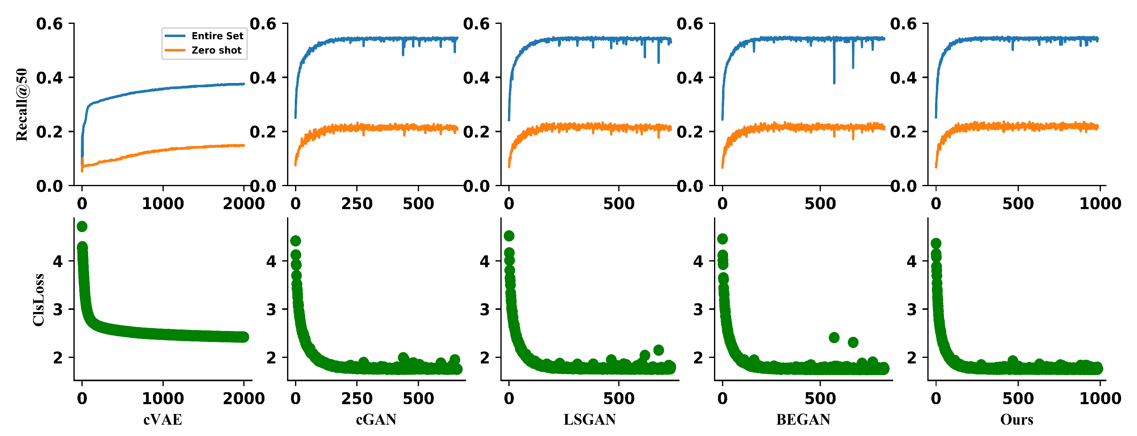
Effect of Generation Methods. An important question about our approach is whether the generative methods succeed in mapping label embedding to suitable coefficients for relationship. In order to answer this question, the evolution of the relationship classification loss which is a function of epochs is shown in Figure 5. In general, the classification loss $l_{rel}$ decreases steadily over training, showing the success of our model in mapping.

Another relevant question is whether our method keep convergent or not for generating coefficients, compared to the other methods. Figure 5 shows the Recall@50 of relationship detection as the function of epochs with different generation methods, e.g., Boundary Equilibrium Generative Adversarial Networks(BEGAN) [41], Least Squares Generative Adversarial Networks(LSGAN) [42] and original GAN [20], which are trained with the same setting and structure. In particular, LSGAN and BEGAN have more prone to training crashes and produce more serious training instability results even compared with the original GAN. While the stable training trend and loss convergence during the training of WGAN is observed, similar conclusions are also drawn from the recent work [43].

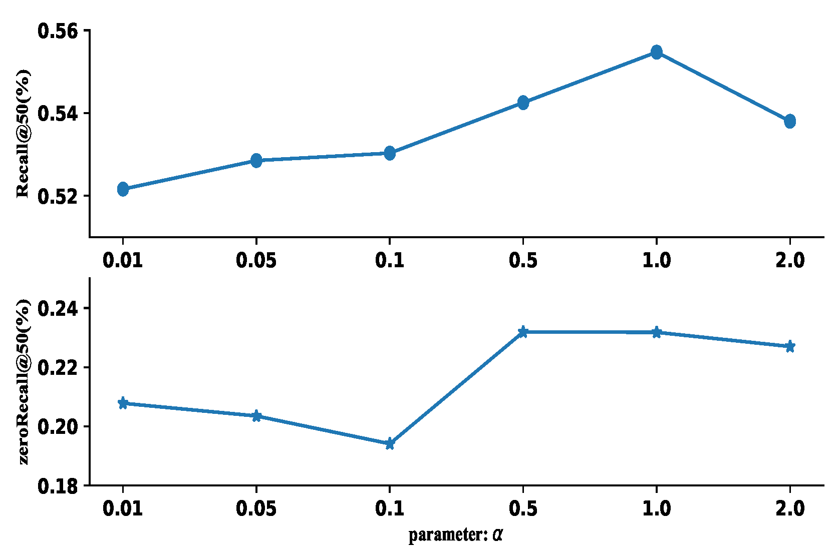
After verifying that our method leads to more stable training performance than the other methods, the generalization ability of different methods is another critical problem. Hence, the results of predicate detection on entire set and zero-shot with different generative models are compared in

Table 3. Different Generation Methods in Predicate Detection.

Methods	Entire Set.	Zero-Shot.
	R@100/50	R@100/50
cVAE [44]	37.5	14.8
cGAN [20]	54.5	20.8
LSGAN [42]	52.9	20.7
BEGAN [41]	54.2	21.6
CCEF	55.5	23.2

. In both the entire set and zero-shot setting, our model has the best performance for generating highly suitable coefficients. And the GAN models have the better performance of generalization on both entire set and zero-shot and converge faster than cVAE. We conjecture that VAE tends to produce blurred results and leads to the inaccurate coefficients. In addition, the generalization ability of our model is also affected by the balance term $\alpha$ in (9), as shown in Figure 6.

Comparison with Attention Methods. To tackle the problem of relationship-independent visual appearance, another promising approach is attention mechanism, which encourages the network to focus on the discriminative regions of feature map during extracting the visual features. Therefore, the detection results of existing attention methods with our excitation approach and choose ResNet-50 [45] as the feature extractor in Figure 2 are compared to determine the effect of visual feature distributions.

The experimental results in

Table 4. Predicate detection results of different attention methods with ResNet-50 as feature extractor.

Methods	Entire Set.	Zero-Shot.
	R@100/50	R@100/50
Appearance	49.2	17.6
VSA-Spatial [38]	43.5	14.1
CAI-Direct [7]	50.9	18.5
CAI-Context [7]	52.0	19.3
CCEF	56.2	25.2

show that most attention mechanisms are effective but inappropriate weight assignments may not contribute to the final detection, e.g., “VSA-Spatial”, which always focuses on the center of object region. These experimental results also demonstrate that our excitation approach, which make the network focus on the discriminative feature of visual relationship appearance, is more effective than attention methods. Besides, the experimental results in Table 1 and Table 4 show that our contextual coefficients are able to be suitable for various visual feature distributions and ResNet features are stronger than VGG, which is expected.

6. Conclusions

In this paper, we proposed the contextual coefficients excitation feature (CCEF), an dynamic feature recalibration on context for VRD task. Instead of attention mechanism, we use conditional WGAN to learn the importance distribution of visual features, and use semantic description as constraints. Zero-shot experiments show that the features distribution learned by WGAN have better generalization ability for identifying new relationships. In future, we will further study the joint adversarial learning of visual and semantic representation, so as to improve the ability of Zero-Shot prediction in different task.

References

- Zhou, P.; Ni, B.; Geng, C.; Hu, J.; Xu, Y. Scale-transferrable object detection. In Proceedings of the IEEE Conference on Computer Vision and Pattern Recognition, Salt Lake City, UT, USA, 18–22 June 2018; pp. 528–537. [Google Scholar]
- Krizhevsky, A.; Sutskever, I.; Hinton, G.E. ImageNet Classification with Deep Convolutional Neural Networks; Communications of the ACM: New York, NY, USA, 2017; pp. 84–90. [Google Scholar]
- Wang, H.; Wang, Q.; Gao, M.; Li, P.; Zuo, W. Multi-scale location-aware kernel representation for object detection. In Proceedings of the IEEE Conference on Computer Vision and Pattern Recognition, Salt Lake City, UT, USA, 18–22 June 2018; pp. 1248–1257. [Google Scholar]
- Liu, Y.; Wang, R.; Shan, S.; Chen, X. Structure inference net: Object detection using scene-level context and instance-level relationships. In Proceedings of the IEEE Conference on Computer Vision and Pattern Recognition, Salt Lake City, UT, USA, 18–22 June 2018; pp. 6985–6994. [Google Scholar]
- Deng, J.; Dong, W.; Socher, R.; Li, L.-J.; Li, K.; Li, F.-F. Imagenet: A large-scale hierarchical image database. In Proceedings of the 2009 IEEE Conference on Computer Vision and Pattern Recognition, Miami, FL, USA, 20–25 June 2009; pp. 248–255. [Google Scholar]
- Zhou, G.; Zhang, M.; Ji, D.H.; Zhu, Q. Tree kernel-based relation extraction with context-sensitive structured parse tree information. In Proceedings of the 2007 Joint Conference on Empirical Methods in Natural Language Processing and Computational Natural Language Learning (EMNLP-CoNLL), Prague, Czech Republic, 28–30 June 2007; pp. 728–736. [Google Scholar]
- Zhuang, B.; Liu, L.; Shen, C.; Reid, I. Towards context-aware interaction recognition for visual relationship detection. In Proceedings of the IEEE International Conference on Computer Vision, Venice, Italy, 22–29 October 2017; pp. 589–598. [Google Scholar]
- Lu, C.; Krishna, R.; Bernstein, M.; Fei-Fei, L. Visual relationship detection with language priors. In European Conference on Computer Vision; Springer: Cham, Switzerland, 2016; pp. 852–869. [Google Scholar]
- Yu, R.; Li, A.; Morariu, V.I.; Davis, L.S. Visual relationship detection with internal and external linguistic knowledge distillation. In Proceedings of the IEEE International Conference on Computer Vision, Venice, Italy, 22–29 October 2017; pp. 1974–1982. [Google Scholar]
- Zellers, R.; Yatskar, M.; Thomson, S.; Choi, Y. Neural motifs: Scene graph parsing with global context. In Proceedings of the IEEE Conference on Computer Vision and Pattern Recognition, Salt Lake City, UT, USA, 18–22 June 2018; pp. 5831–5840. [Google Scholar]
- Arjovsky, M.; Chintala, S.; Bottou, L. Wasserstein gan. arXiv 2017, arXiv:1701.07875. [Google Scholar]
- Springenberg, J.T.; Dosovitskiy, A.; Brox, T.; Riedmiller, M. Striving for simplicity: The all convolutional net. arXiv 2014, arXiv:1412.6806. [Google Scholar]
- Bilen, H.; Fernando, B.; Gavves, E.; Vedaldi, A.; Gould, S. Dynamic image networks for action recognition. In Proceedings of the IEEE Conference on Computer Vision and Pattern Recognition, Las Vegas, NV, USA, 27–30 June 2016; pp. 3034–3042. [Google Scholar]
- Sadeghi, M.A.; Farhadi, A. Recognition using visual phrases. In Proceedings of the CVPR 2011, Providence, RI, USA, 20–25 June 2011; pp. 1745–1752. [Google Scholar]
- Zhu, Y.; Jiang, S.; Li, X. Visual relationship detection with object spatial distribution. In Proceedings of the 2017 IEEE International Conference on Multimedia and Expo (ICME), Hong Kong, China, 10–14 July 2017; pp. 379–384. [Google Scholar]
- Zhang, H.; Kyaw, Z.; Chang, S.F.; Chua, T.S. Visual translation embedding network for visual relation detection. In Proceedings of the IEEE Conference on Computer Vision and Pattern Recognition, Honolulu, HI, USA, 21–26 July 2017; pp. 5532–5540. [Google Scholar]
- Yin, G.; Sheng, L.; Liu, B.; Yu, N.; Wang, X.; Shao, J.; Change Loy, C. Zoom-net: Mining deep feature interactions for visual relationship recognition. In Proceedings of the European Conference on Computer Vision (ECCV), Munich, Germany, 8–14 September 2018; pp. 322–338. [Google Scholar]
- Yang, J.; Lu, J.; Lee, S.; Batra, D.; Parikh, D. Graph r-cnn for scene graph generation. In Proceedings of the European Conference on Computer Vision (ECCV), Munich, Germany, 8–14 September 2018; pp. 670–685. [Google Scholar]
- Li, Y.; Ouyang, W.; Zhou, B.; Shi, J.; Zhang, C.; Wang, X. Factorizable net: An efficient subgraph-based framework for scene graph generation. In Proceedings of the European Conference on Computer Vision (ECCV), Munich, Germany, 8–14 September 2018; pp. 335–351. [Google Scholar]
- Goodfellow, I.; Pouget-Abadie, J.; Mirza, M.; Xu, B.; Warde-Farley, D.; Ozair, S.; Courville, A.; Bengio, Y. Generative adversarial nets. In Advances in Neural Information Processing Systems; MIT Press: Cambridge, MA, USA, 2014; pp. 2672–2680. [Google Scholar]
- Gulrajani, I.; Ahmed, F.; Arjovsky, M.; Dumoulin, V.; Courville, A.C. Improved training of wasserstein gans. In Advances in Neural Information Processing Systems; Curran Associates Inc.: Red Hook, NY, USA, 2017; pp. 5767–5777. [Google Scholar]
- Kossaifi, J.; Tran, L.; Panagakis, Y.; Pantic, M. Gagan: Geometry-aware generative adversarial networks. In Proceedings of the IEEE Conference on Computer Vision and Pattern Recognition, Salt Lake City, UT, USA, 18–22 June 2018; pp. 878–887. [Google Scholar]
- Yu, J.; Lin, Z.; Yang, J.; Shen, X.; Lu, X.; Huang, T.S. Generative image inpainting with contextual attention. In Proceedings of the IEEE Conference on Computer Vision and Pattern Recognition, Salt Lake City, UT, USA, 18–22 June 2018; pp. 5505–5514. [Google Scholar]
- Mirza, M.; Osindero, S. Conditional generative adversarial nets. arXiv 2014, arXiv:1411.1784. [Google Scholar]
- Choi, Y.; Choi, M.; Kim, M.; Ha, J.W.; Kim, S.; Choo, J. Stargan: Unified generative adversarial networks for multi-domain image-to-image translation. In Proceedings of the IEEE Conference on Computer Vision and Pattern Recognition, Salt Lake City, UT, USA, 18–22 June 2018; pp. 8789–8797. [Google Scholar]
- Brock, A.; Donahue, J.; Simonyan, K. Large scale gan training for high fidelity natural image synthesis. arXiv 2018, arXiv:1809.11096. [Google Scholar]
- Peng, Y.; Qi, J. CM-GANs: Cross-modal generative adversarial networks for common representation learning. ACM Trans. Multimedia Comput. Commun. Appl. 2019, 15, 22. [Google Scholar] [CrossRef]
- Wang, J.; Li, X.; Yang, J. Stacked conditional generative adversarial networks for jointly learning shadow detection and shadow removal. In Proceedings of the IEEE Conference on Computer Vision and Pattern Recognition, Salt Lake City, UT, USA, 18–22 June 2018; pp. 1788–1797. [Google Scholar]
- Zhang, G.; Kan, M.; Shan, S.; Chen, X. Generative adversarial network with spatial attention for face attribute editing. In Proceedings of the European Conference on Computer Vision (ECCV), Munich, Germany, 8–14 September 2018; pp. 417–432. [Google Scholar]
- Zhao, B.; Chang, B.; Jie, Z.; Sigal, L. Modular generative adversarial networks. In Proceedings of the European Conference on Computer Vision (ECCV), Munich, Germany, 8–14 September 2018; pp. 150–165. [Google Scholar]
- Bucher, M.; Herbin, S.; Jurie, F. Generating visual representations for zero-shot classification. In Proceedings of the IEEE International Conference on Computer Vision, Venice, Italy, 22–29 October 2017; pp. 2666–2673. [Google Scholar]
- Felix, R.; Kumar VB, G.; Reid, I.; Carneiro, G. Multi-modal cycle-consistent generalized zero-shot learning. In Proceedings of the European Conference on Computer Vision (ECCV), Munich, Germany, 8–14 September 2018; pp. 21–37. [Google Scholar]
- Xian, Y.; Lorenz, T.; Schiele, B.; Akata, Z. Feature generating networks for zero-shot learning. In Proceedings of the IEEE Conference on Computer Vision and Pattern Recognition, Salt Lake City, UT, USA, 18–22 June 2018; pp. 5542–5551. [Google Scholar]
- Mikolov, T.; Chen, K.; Corrado, G.; Dean, J. Efficient estimation of word representations in vector space. arXiv 2013, arXiv:1301.3781. [Google Scholar]
- Bordes, A.; Usunier, N.; Garcia-Duran, A.; Weston, J.; Yakhnenko, O. Translating embeddings for modeling multi-relational data. In Advances in Neural Information Processing Systems; Curran Associates Inc.: Red Hook, NY, USA, 2013; pp. 2787–2795. [Google Scholar]
- Kingma, D.P.; Ba, J. Adam: A method for stochastic optimization. arXiv 2014, arXiv:1412.6980. [Google Scholar]
- Yang, X.; Zhang, H.; Cai, J. Shuffle-then-assemble: Learning object-agnostic visual relationship features. In Proceedings of the European Conference on Computer Vision (ECCV), Munich, Germany, 8–14 September 2018; pp. 36–52. [Google Scholar]
- Han, C.; Shen, F.; Liu, L.; Yang, Y.; Shen, H.T. Visual spatial attention network for relationship detection. In Proceedings of the 2018 ACM Multimedia Conference on Multimedia Conference, Seoul, Korea, 22–26 October 2018; pp. 510–518. [Google Scholar]
- Jae Hwang, S.; Ravi, S.N.; Tao, Z.; Kim, H.J.; Collins, M.D.; Singh, V. Tensorize, factorize and regularize: Robust visual relationship learning. In Proceedings of the IEEE Conference on Computer Vision and Pattern Recognition, Salt Lake City, UT, USA, 18–22 June 2018; pp. 1014–1023. [Google Scholar]
- Peyre, J.; Sivic, J.; Laptev, I.; Schmid, C. Weakly-supervised learning of visual relations. In Proceedings of the IEEE International Conference on Computer Vision, Venice, Italy, 22–29 October 2017; pp. 5179–5188. [Google Scholar]
- Berthelot, D.; Schumm, T.; Metz, L. Began: Boundary equilibrium generative adversarial networks. arXiv 2017, arXiv:1703.10717. [Google Scholar]
- Mao, X.; Li, Q.; Xie, H.; Lau, R.Y.; Wang, Z.; Paul Smolley, S. Least squares generative adversarial networks. In Proceedings of the IEEE International Conference on Computer Vision, Venice, Italy, 22–29 October 2017; pp. 2794–2802. [Google Scholar]
- Lucic, M.; Kurach, K.; Michalski, M.; Gelly, S.; Bousquet, O. Are gans created equal? A large-scale study. In Advances in Neural Information Processing Systems; Curran Associates Inc.: Red Hook, NY, USA, 2018; pp. 700–709. [Google Scholar]
- Bao, J.; Chen, D.; Wen, F.; Li, H.; Hua, G. CVAE-GAN: Fine-grained image generation through asymmetric training. In Proceedings of the IEEE International Conference on Computer Vision, Venice, Italy, 22–29 October 2017; pp. 2745–2754. [Google Scholar]
- He, K.; Zhang, X.; Ren, S.; Sun, J. Deep residual learning for image recognition. In Proceedings of the IEEE Conference on Computer Vision and Pattern Recognition, Las Vegas, NV, USA, 27–30 June 2016; pp. 770–778. [Google Scholar]
Figure 1.
Visualization of relationship detection results. (a) is the original image. (b,d) are the subject and object original visual features obtained from fine-tuned CNN. (c,e) are our focal visual representation compared with (b,d). (f) is the detection result of these two settings.
Figure 2.
Overview of our visual relationship detection framework. A set of detected object regions are first cropped from input image and fed into feature extractor, a base CNN network, to extract the visual features. Then, CCEF is produced by exciting visual features rely on contextual coefficients, which are carried out by the generated-label coefficients and spatial coefficients. The relationship are represented by subtracting objects from subjects.
Figure 3.
The structure of our conditional WGAN. Our WGAN minimizes the relationship predication loss over the generated coefficients and the Wasserstein distance with gradient penalty to ensure the stability of GAN.
Figure 4.
Performance of different sizes of training examples. “CCEF” and “Appearance” have the same setting as Section 4.
Figure 5.
Evolution of and convergence of the Recall@50 in terms of epochs for the contextual coefficients from the different methods: cVAE, cGAN, LSGAN, BEGAN and ours.
Figure 6.
Effectiveness of contextual coefficients with various settings in (9) for predicate detection.