Nonlinear Aeroelastic in-Plane Behavior of Suspension Bridges under Steady Wind Flow


1
International Research Center on Mathematics and Mechanics of Complex Systems, University of L’Aquila, 67100 L’Aquila, Italy
2
Department of Civil, Construction-Architectural and Environmental Engineering, University of L’Aquila, 67100 L’Aquila, Italy
*
Author to whom correspondence should be addressed.
†
These authors contributed equally to this work.
Appl. Sci. 2020, 10(5), 1689; https://0-doi-org.brum.beds.ac.uk/10.3390/app10051689
Submission received: 9 January 2020
/
Revised: 18 February 2020
/
Accepted: 23 February 2020
/
Published: 2 March 2020
(This article belongs to the Special Issue Bridge Dynamics)
Abstract
:The nonlinear aeroelastic behavior of suspension bridges, undergoing dynamical in-plain instability (galloping), is analyzed. A nonlinear continuous model of bridge is formulated, made of a visco-elastic beam and a parabolic cable, connected each other by axially rigid suspenders, continuously distributed. The structure is loaded by a uniform wind flow which acts normally to the bridge plane. Both external and internal damping are accounted for the structure, according to the Kelvin-Voigt rheological model. The nonlinear aeroelastic effects are evaluated via the quasi-static theory, while structural nonlinearities are not taken into account. First, the free dynamics of the undamped bridge are addressed, and the natural modes determined. Then, the nonlinear equations ruling the dynamics of the aeroelastic system, close to the bifurcation point, are tackled by the Multiple Scale Method. This is directly applied to the partial differential equations, and provides the finite-dimensional bifurcation equations. From these latter, the limit-cycle amplitude and its stability are evaluated as function of the mean wind velocity. A case study of suspension bridge is analyzed.
1. Introduction
Suspension bridges are long, slender and flexible structures which are very sensitive to dynamic actions induced by wind, which potentially cause a variety of instability phenomena. The importance of wind-resistant design for these structures has been highly recognized and has led to many research works and investigations on bridge aerodynamics. Some historical views of long-span bridge aerodynamics are presented in [1,2].
The first studies were addressed on the dynamic of suspended cables, pertinent to suspension bridges but without the inclusion of the stiffening girder, see Irvine and Caughey [3] and Irvine [4]. Since the 1980s, starting with Hagerdon and Schafer [5] and Luongo et al. [6,7], there has been a large number of studies on the free and forced nonlinear vibrations of suspended cables (see the review of Rega, in [8,9]). In particular, some papers investigated wind-induced aeroelastic instabilities, as [10,11,12].
After the Tacoma Narrows Bridge failure in 1940, major efforts were made to understand the dynamic of suspension bridge, including the effects of the stiffening girder. Bleich [13] modeled the stiffening girder as a flexural beam attached to the elastic cables by inextensible hangers. Additional contributions to the continuum model were made by Pugsley [14]. Abdel-Ghaffar [15] extended the approach to include coupled vertical–torsional vibrations and the effects of cross-sectional distortion. Hayashikawa and Watanabe [16] and Kim et al. [17] enriched the linearized continuum model including the effects of shear deformation and rotary inertia of the stiffening girder, by concluding that these effects are relatively small and only affect the higher modes of vibration. More recently, in [18] the classical continuum model for the free linear vertical vibrations of a suspension bridge is re-examined.
Remarkable attention has been addressed to the aeroelastic behavior of long-span bridges, and especially to the aeroelastic instability, as galloping (1 d.o.f) or flutter (2 d.o.f.), which may cause catastrophic effects, like in the famous Tacoma Narrows bridge. The modern era of bridge aeroelasticity was launched by Farquharson [19]. Bleich [20], for the first time, analyzed the bridge flutter behavior by exploiting the Theodorsen theory of thin airfoils, with the potential flow assumption. During the same period, empirical formulas were proposed, based on the bridge structural properties only, to directly obtain the critical flutter wind velocity without involving any consideration of the flow field (e.g., [21]). Scanlan and his colleagues [22] introduced a semiempirical linearized analysis, referred to as “unsteady theory”, based on the so-called “flutter derivatives”, which is nowadays still popular among researchers. In [23], advances in aeroelastic analyses of suspension bridges are described, with focus on the numerical simulations carried out for a long-span suspension bridge, using finite difference and discrete vortex methods. More recently, many linear and nonlinear aeroelastic analyses for cable-supported bridges were developed, e.g., [24,25,26,27,28]. In [24], a nonlinear aerodynamic force model and associated time domain analysis is performed to predict the aeroelastic response of bridges under turbulent winds. In [25], a numerical method for full-bridge aeroelasticity is presented, based on unsteady cross-sectional wind loads and on the finite-element modeling of the structure. In [26], a fully nonlinear model of suspension bridge is proposed to describe overall three-dimensional motions. Torsional-divergence and flutter are studied by numerical methods, able to tackle the coupled nonlinear partial-differential equations of motion. In [27], after a review of the existing linear and nonlinear analyses, two advanced nonlinear models are introduced to study the aeroelastic effects under smooth/turbulent wind conditions: (a) artificial neural network and, (b) Volterra series-based models. In [28], the limit-cycle oscillations exhibited by long-span suspension bridges in post-flutter condition are investigated. The governing aeroelastic partial differential equations are solved by the Faedo-Galerkin method.
Most of the studies about the aerodynamic instability of the bridge were devoted to flutter phenomena, according to which the aeroelastic instability involves two coalescent modes, one torsional, the other flexural. This is the case of bridges with low torsional stiffness, for which the natural torsional and flexural frequencies are close each other, prone to coalesce under aerodynamic excitation. On the contrary, bridges with high torsional stiffness (e.g., box-girder bridges) have the fundamental torsional frequency much larger than the flexural one, so that the aerodynamic instability exclusively occurs in the flexural mode (galloping instability). This class of bridges also attracted some interest, justified by the fact that, after the Tacoma collapse, many existing bridges were torsionally stiffened and the new bridges were designed with stiffer trusses (e.g., the Verrazzano bridge in New York, Tago bridge in Lisbon or the Japanese bridge Akashi Kaikyo). Many works in literature dealt with the galloping instability separately in the beam (see, e.g., [29,30,31,32,33]) and in the cable (see, e.g., [34,35,36,37]). With reference to the class of bridges with high torsional stiffness, the interest was addressed mainly to the galloping control (see, e.g., [38,39,40]).
In this paper, the interest is focused on galloping of suspension bridges. Differently from the current research trend, according to which fine discretized models are used to analyze particular bridges, here the aeroelastic behavior is investigated via a continuous model, in order to study families of bridges, and to identify the key dimensionless parameters which govern the mechanical behavior. The main innovative aspect, therefore, relies in directly attacking the continuous problem by perturbation methods (similarly to what done by the same authors in [41]), which leads to approximate formulae, suitable for preliminary design. A simple continuous model of suspension bridge, subjected to steady wind flow, is proposed to analyze the aeroelastic in-plain instability (galloping). Linear visco-elastic beam and cable are considered, coupled by vertical suspenders, modeled as axially rigid links uniformly distributed. Both external and internal damping are accounted, both for the beam and cable, according to the Kelvin-Voigt rheological model. A steady and uniform wind flow is applied exclusively to the beam. The aeroelastic effects of the wind are evaluated via the classical quasi-static theory (a discussion about strengths and weaknesses of the method is reported in [42]). First, the linear free dynamic of the undamped model is studied; then, the nonlinear bifurcation problem is tackled by the Multiple Scale Method (MSM) which naturally reduces the infinite-dimensional system to the proper finite-dimensional Center Manifold. From the bifurcation equation, the limit cycles and their stability are evaluated as function of the mean wind velocity. The asymptotic results are validated via numerical time-integration of ordinary differential equations derived by in-space finite differences. A case study of suspension bridge is analyzed.
The paper is organized as follows. In Section 2, a continuous visco-elastic model of standard single-span suspension bridge under uniformly distributed steady wind flow, is formulated. In Section 3, the free dynamic of the undamped problem is addressed. In Section 4 the Multiple Scale Method is directly applied to the partial differential equations, to get the bifurcation equation governing the motion close to a Hopf bifurcation. In Section 5, a finite-dimensional model is formulated. In Section 6, the numerical outcomes are presented. Finally, in Section 7 the main findings of the work are summarized. An Appendix A, containing details about damping parameter identification, closes the paper.
2. Continuous Model
A standard single-span suspension bridge is considered, consisting of a main cable, a stiffening girder, equispaced hangers (or suspenders) and two supporting towers (Figure 1).
The main cable, modeled as uniform, elastic and perfectly flexible (no bending stiffness) is connected to the tip of towers, taken to be infinitely rigid. The girder is modeled as an Euler-Bernoulli beam, simply supported at both ends. The structure is subjected to a steady and uniform wind flow of velocity U. The dynamics of the structure are studied in the vertical plane, while the out-of-plane motions are ignored.
The main cable is modeled according the Irvine’s theory [3], holding for sag-to-span ratios up to about 1:10. The cable assumes a parabolic profile under the initial dead load, and experiences vibrations in which the tangent component is statically condensed. Beam and cable are coupled by vertical hangers, here assumed to be massless, inextensible and continuously distributed along the span of the bridge (curtain of hangers) which apply equal and opposite distributed reactive forces to the two substructures.
2.1. Equations of Motion
Kinematics of the beam are assumed to be linear; nonlinearities are accounted for in the description of the aerodynamic forces only. The current configuration, both of the beam and of the cable, is described by the common transverse displacement field , with an abscissa along the beam axis and t the time. The equations ruling the in-plane motion, obtained eliminating the reactive forces between the cable and the beam equations, are:
where is the flexural stiffness of the beam, is the axial stiffness of the cable, and and are the beam and cable linear mass density, respectively (and therefore the total bridge linear mass density is ). Here is the prestress of the cable, assumed constant on s, and , with g the acceleration gravity, is the prestress curvature, also assumed to be constant. The integral term accounts for the increment of tension, which depends on the time only.
In Equation (1), the non-inertial contribution of the external loads are decomposed in the damping and aerodynamic parts, as:
where the subscripts refer respectively the beam and cable.
2.2. Damping Forces
A damping continuous model, accounting for both external damping (due to firm air-structure interaction) and internal damping (due to material dissipation), is used. This approach is different from that usually followed in literature, in which an ‘overall’ damping is attributed to the modes of the discrete system on experimental (or of literature) ground.
The contribution of the internal damping is related to two different physical mechanisms (see [37]): (a) elongation of the longitudinal fibers, both in cable and in beam, and (b) internal friction of the prestressed fibers of the cable. By adopting the Kelvin-Voigt model for mechanism (a), the elastic modulus must be replaced by with an internal viscous damping coefficient, having physical dimensions of a time. By adopting the same rule for mechanisms (b), the pretension must be replaced by . In symbols:
Accordingly, the time-differential damping operator is proportional to the elasto-geometric stiffness operator. Such a type of damping is usually referred as proportional, or Raleigh model, in the context of the finite-dimensional systems.
The external damping is modeled by forces proportional to velocities, as:
in which and are beam and cable external damping coefficients, from which is the coefficient of total external damping.
Note that the damping model introduced here is able to distinguish the beam and cable contributions. The four damping parameters can be calibrated to reproduce modal damping of as many modes.
2.3. Aerodynamic Forces
The aerodynamic part of the load is caused by the wind, which blows orthogonally to the plane of bridge, with a steady velocity U. It triggers forces on the beam and on the cable, acting both in-plane and out-of-plane of the structure. Due to the higher out-of-plane stiffness of the beam and to the smaller dimensions of the cable (which, being of circular shape, is exclusively subjected to drag forces), only in-plane forces acting on the beam are taken into account.
The quasi-static theory (see [29]) is used here to express such forces. The choice is corroborated by the discussion carried out in [28], where it is stated that: (a) the use of a nonlinear quasi-steady theory is justified in the range of low reduced frequencies, in which long-span bridges are expected to fall; and, (b) the previsions of the quasi-steady model are conservative, a few percent lower than those of a fully unsteady model. In particular, it is known that (see e.g., [43,44]), the quasi-steady assumption is valid only if the main frequency of periodic components of fluid forces, associated with vortex-shedding, is well above the dominant structural frequency, i.e., , where is the natural frequency of the crosswind vibration mode of the structure and , with the Struhal number and b the deck width. The occurrence of the frequency condition will be verified in the numerical application. When the inequality is not satisfied, it is needed to resort to a non-steady theory. However, while this latter is well codified in the linear range, few studies concern nonlinear dynamics (e.g., [44,45,46]).
In the framework of the quasi-steady theory, the forces depend on the structural velocity only (not on the frequency of the oscillations), as result of the aeroelastic interaction. By expressing them in series of powers of the ratio, by assuming the cross-section is symmetric with respect the horizontal axis, and truncating the series to the fifth order, they read:
Here, is the air mass density, are dimensionless aerodynamic coefficients (depending on the shape of the cylinder cross-section), D is a transverse characteristic length, and ( ) are dimensional coefficients, introduced to simplify the notation.
2.4. Dimensionless Equation of Motion
By introducing the following non-dimensional quantities:
and parameters:
the equations of motion are recast in non-dimensional form:
In Equation (8), prime and dot denote differentiation with respect to non-dimensional space and time, respectively, and the tilde is dropped for convenience. It is noticed that nonlinearities are only due to aerodynamics.
The dimensionless parameter is the well-known Irvine-Caughey parameter [3], accounting for geometric and mechanical properties of the cable. The dimensionless parameter (also used in [13,47,48] and others), describes the beam-to-cable stiffness ratio. For long bridges, it tends to zero, so that such bridges behave as a cable with an appended mass. However, still in this case, the parameter causes the occurrence of boundary layers close to the constraints and the point-loads, where the flexural behavior cannot be neglected. In this paper, attention will be devoted to bridges of medium length, in which the role of the beam is not negligible, as it will be discussed soon. A parametric study about the influence of both parameters on the free dynamic of the bridge is carried out in [18].
3. Linear Undamped Oscillations
First, the free dynamics of the undamped problem are addressed to evaluate the natural frequencies and modes. Although this problem has already been solved in literature (see, e.g., [13,18]), it is shortly resumed here for completeness.
The relevant equations of motion are:
By separating the variables as , a space eigenvalue problem follows:
whose eigensolutions , , are the natural frequencies and modes, respectively. Due to the symmetry of the structure with respect , the modes are of anti-symmetric and symmetric types.
3.1. Anti-Symmetric Modes
In the anti-symmetric modes, the integral term in the equations disappears (no change of tension occurs), so that the system behaves as a string, stiffned by an in-parallel beam. Accordingly:
and
are the nth anti-symmetric eigenpair. It is independent of , i.e., of the elasto-geometric properties of the cable, but depends on the parameter , i.e., on the stiffness ratio. It is worth noticing that the frequency of the first mode () nearly doubles with respect to that of the string when . It is concluded that the stiffening effect of the girder is significant when .
3.2. Symmetric Mode
The nth symmetric natural mode is found to be:
where the following definitions hold for the coefficient :
and is a normalization factor, such that . In Equation (13), , are frequency-dependent wave-numbers, defined as follows:
The unknown squared frequency is found as a root of the transcendent characteristic equation:
Therefore, an explicit expression for the natural frequency of the symmetric modes cannot be provided.
4. Aeroelastic Stability Analysis
To investigate the behavior of the structure in the nonlinear field and close to the dynamic bifurcation, a nonlinear analysis is carried out. To solve the nonlinear problem, Equation (8), the asymptotic Multiple Scale Method (MSM) is used, by directly attacking the partial differential equations of motion. The method consists in expanding the dependent variables in a formal series of a small perturbation parameter (to be reabsorbed at the end of the procedure), as well as introducing independent time scales. Substitution of these expansions in the nonlinear equations and separation of terms of different orders, lead to linear differential equations to be solved in sequence. Here, the MSM is used as reduction method, as an alternative to the Center Manifold Method ([49,50]). It provides a bifurcation equation ruling the dynamic on a center manifold of finite dimension (two-dimensional in the case of simple Hopf bifurcation).
4.1. Bifurcation Equation
According to the MSM, a small dimensionless parameter is introduced by a suitable ordering of variables and parameters. First, the displacement is rescaled as , so that is of the order of the amplitude of motion. Then, damping and aerodynamic coefficients are rescaled as: , , , , , , i.e., nonlinear coefficients are taken much larger than the linear ones (as suggested by the numerical application illustrated ahead), in order linear and nonlinear aerodynamic forces appear at the same level in the perturbation scheme. Moreover, independent time-scales , , ..., are introduced, so that . Hence, by exploiting the chain rule, the following formal expansions for the time differential operators hold:
in which , . Finally, the independent variable is expanded in series of as:
By introducing rescaling and expansions in the equations of motion, and collecting the coefficients of the different powers of , the following perturbation equations are derived.
Order :
Order :
The generating problem, Equation (19), admits the monomodal solution:
in which is an unknown complex modulating function, c.c. stands for complex conjugate terms, and is a real eigenpair of the undamped and unloaded model, determined in Section 3.
When the -order problem, Equation (20), is considered, damping and aerodynamics terms appear on the right hand side of the equation, to be evaluated via Equation (21). Here, the internal damping would trigger point-moments at the boundaries, equal to ; however, this last contribution is zero, because of the lower-order conditions . Equation (20) therefore read:
where NRT stands for Non Resonant Terms, and
Since the operator is singular (i.e., it admits a nontrivial homogeneous solution), the non-homogeneous problem cannot be solved for a generic know term. Therefore, a compatibility (or solvability) condition, known as Fredholm alternative, has to be enforced on it. This condition requires the -frequency forcing terms are orthogonal to the kernel of the self-adjoint operator, i.e.,
A detailed discussion on solvability conditions is provided in [51,52], in the framework of perturbation methods.
From Equation (24), an ordinary differential equation on the scale is obtained for the amplitude. By coming back to the true time t via backward rescaling, the equation assumes the well-known normal form for the Hopf bifurcation, i.e.,
where the real quantities are defined as follows:
Finally, by letting , and separating real and imaginary parts in Equation (25), the real form of the bifurcation equation is derived:
Equation (27)-b supplies , since structural nonlinearities, that would be responsible for phase modulations, have been ignored. The steady solutions of Equation (27)-a are periodic solutions for the original system; the periodic solutions are quasi-periodic solutions for the original system. Due to the normalization adopted for the natural modes, the real amplitude a describes: (a) the maximum modulus of the displacement in the anti-symmetric modes, and, (b) the displacement at in the symmetric modes.
4.2. Linear Stability Analysis and Critical Wind Velocity
The dynamic of the bridge, close to the rest position, is ruled by the linear part of Equation (25), which admits the solution , where . The position is asymptotically stable if and unstable if The condition of incipient instability occurs for , that is for the wind velocity getting its critical (galloping velocity) value:
at which a Hopf bifurcation occurs. Since, from Equation (26), (dissipative damping), bifurcation occurs only if (self-exciting aerodynamics, entailing ). Once the wind direction has been fixed, this last condition occurs only for some cross-section shape (just said, aerodynamically unstable).
The critical wind velocity depends on the mode at which the bridge is oscillating, each velocity being associated to each mode. The lowest critical velocity is associated with the lowest mode (at which the internal damping is minimum), which can be either symmetric (Equation (13)) or anti-symmetric (Equation (11)). For this latter, an explicit formula can be derived, namely:
The beneficial influence of the flexural stiffness should be noticed, since the critical wind velocity increases with . This is due to the fact that the internal damping is proportional to the stiffness, according to the Kelvin-Voigt model adopted.
4.3. Limit-Cycle Analysis
Steady non-trivial solutions of the bifurcation Equation (27)-a describe periodic oscillations occurring on limit-cycles. By letting and solving the biquadratic algebraic equation, two explicit solutions are found (to within an unessential sign):
where:
They describe two velocity-dependent branches (denoted by the ± index) of the bifurcation diagram . Depending on u, two, one o zero nontrivial real solutions exist. In order to discuss the number of solutions, here the interesting case in which and is considered, which entails and . This case is typical, for example, of rectangular cross-sections with a 2:1 aspect ratio (see [29,31]), according which the qualitative galloping response is plotted in Figure 2.
Preliminary, it is observed that is negative in the subcritical range and positive in the supercritical range. Then, the sign of the discriminant is discussed. Let:
be the value of velocity at which the discriminant vanishes, i.e. . Since , it follows that:
- when , it is , so that no real solutions exist;
- when , it is ; however, due , it is , so that both the and roots are real;
- when , in addition to , it is also ; consequently, , which entails that only is real.
The two branches coalesce at , at which and a turning point manifests itself.
4.4. Stability Analysis
To detect stability of the periodic solutions, the 1-dimensional dynamical system described by Equation (27)-a is perturbed, by letting , where is a small deviation from the steady solution solution . By linearizing in the perturbation, the following variational equation is obtained:
which decides about stability of . From this, by using Equation (30), the following conclusions are derived:
- the lower non-trivial solution is unstable in its domain of existence ;
- the upper non-trivial solution is stable in its domain of existence .
By summarizing (Figure 2), a subcritical Hopf bifurcation occurs at . Here, the trivial solution loses stability, and a family of unstable limit cycles of amplitude bifurcates, whose existence is limited to a portion of the subcritical range. Indeed, at , a turning point modifies unstable to stable cycles, which extend their existence to the supercritical range. As a consequence, if the wind velocity is quasi-statically increased from below through the rest position loses stability and the system jumps from zero to a finite value . A reverse jump occurs at when the wind velocity is decreased from above. An hysteresis can occur for wind velocity periodically changed. Such a behaviour is related to the opposite signs of the aerodynamic coefficients, and , causing a change of the qualitative behaviour of the system, namely: (i) at small amplitudes the cubic terms in the motion Equation (8) prevails over the quintic term; (ii) at higher amplitudes, the opposite occurs. This phenomenon is known in literature as “hard loss of stability”, and observed in several different problems (see, e.g., [53], where the effects of the nonlinear damping on the post-critical behavior of the Ziegler’s column are discussed).
5. Finite-Dimensional Model
Aimed to validate asymptotic results, a finite-dimensional model of bridge for galloping analysis is formulated. The finite-difference method is applied to transform the partial integro-differential Equation (8) into a set of ordinary differential equations, to be numerically integrated for given initial conditions.
The space domain (changed in for simplicity) is divided in equispaced subintervals of amplitude . The following notation is adopted:
in which two external nodes, , have been introduced.
The space derivatives are expressed via the central finite differences:
and the integral term via the trapezoidal rule:
in which the boundary conditions have been accounted for. The field equation in (8), accordingly, becomes:
and the boundary equations read:
6. Numerical Results
The behavior of the long-span suspension bridges is often well-described by the cable only. Here, however, the focus is addressed to cases in which the beam significantly influences the overall mechanics, as it happens when the dimensionless parameter is of order , (see, e.g., [13,18,48]). Therefore, a case study is considered: (a) the geometrical and mechanical characteristics are m, Nm, N, kg/m and kg/m; (b) the prestress is evaluated as , where m is the cable sag; (c) the damping ratio is taken as in the antisymmetric mode, and in the symmetric mode (corresponding to s, Ns/m, s, and Ns/m, whose calibration is shown in Appendix A). A rectangular boxed cross-section of dimension m (and so with an aspect ratio 2:1) is assumed for the beam. The aerodynamic dimensionless coefficients in Equation (5) are drawn from literature (obtained by wind tunnel tests in [30]), namely , , . The air mass density is kg/m.
This example is representative of a class of bridges, whose nondimensional parameters are: , , , , , , , . All numerical values assumed by the parameters are consistent with the ordering performed in the perturbation analysis.
6.1. Linear Stability Analysis
The modal properties of the undamped model were first analyzed. The first natural mode was found to be anti-symmetric (defined by Equation (11) for ) and the corresponding natural frequency is rad/s. The second natural mode was found to be symmetric (defined by Equation (13) for ) and the natural frequency is rad/s (see Figure 3).
The critical conditions corresponding to the antisymmetric and symmetric modes are shown in Table 1. It is observed that the bridge galloped in its first antisymmetric natural mode, in corresponding of which the critical wind velocity assumed the minimum value m/s.
Since the critical velocities corresponding to the antisymmetric and symmetric modes were sufficiently far from each other, nonlinear interactions between modes, leading to multimodal galloping, were excluded.
It was observed that the quasi-steady theory was valid in the case study considered. Indeed, the natural frequency of the first crosswind vibration mode was Hz, while the vortex-shedding frequency was Hz at the critical galloping velocity m/s, according to a Struhal number (as indicated by [54] for a rectangular cross-section with a 2:1 aspect ratio) and a deck width of 2 m. Note that the quasi-steady theory worked mainly due to the narrow width of the cross section.
6.2. Galloping Response
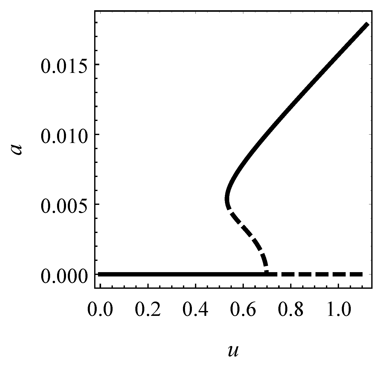
The postcritical behavior relevant to the case study is described by the bifurcation diagram in Figure 4. There, the (dimensionless) steady amplitude a of the anti-symmetric mode, experienced by the bridge on the limit-cycle, is plotted the (dimensionless) wind velocity u. It is seen that, the hard loss of stability caused amplitudes of about of the length (i.e., of the order of 2 m), as far the critical wind velocity was passed.
6.3. Validation by Finite-Dimensional Model
The asymptotic solution was validated against numerical results, relevant to the discretized version (Equations (37) and (38)) of the nonlinear continuous model (Equation (8)). The space interval was divided in subintervals, and numerical integration carried out, via commercial routines, for given initial conditions. Regardless of these latter, after a transient had been exhausted, the motion stabilized either on a limit cycle or comes back to the trivial state. In order to compare the transient motion to that predicted by the MSM via the amplitude , an initial deflection shape coincident with the first natural mode of the undamped bridge was chosen.
Four typical time-histories are shown in Figure 5 for different wind velocities. It was observed that: (a) when (Figure 5a) the motion stabilized on the trivial solution ; (b) when (Figure 5b) the motion stabilized either: (I) on the trivial solution , if the initial condition was sufficiently small, or (II) on a limit cycle of amplitude , if the initial condition was sufficiently large; (c) when (Figure 5c) the motion stabilized on a limit cycle of amplitude . All the time-histories were compared with the numerical integration of the bifurcation Equation (27). It was seen that this latter captured at the best extent the exact (numerical) solution.
To compare the numerical to the asymptotic limit-cycles, the numerical amplitudes were extracted by the recorded time-histories for different wind velocities, and bullets superimposed to the asymptotic bifurcation diagram (see Figure 5d), showing an excellent accordance. Note the power of the perturbation methods in providing accurate predictive formulae (as for the galloping velocity, Equation (29) and for the amplitudes of the limit-cycles, Equation (30)).
7. Conclusions
The nonlinear aeroelastic behavior of suspension bridges, undergoing dynamic in-plain instability (galloping), has been analyzed. A nonlinear continuous model of bridge has been formulated, made of a visco-elastic beam and a parabolic cable, connected each other by axially rigid suspenders, uniformly distributed. A damping continuous model, accounting for both external damping and internal damping (according to the Kelvin-Voigt rheological model), has been used. The structure is loaded by a uniform wind flow, acting normally to its plane. The nonlinear aeroelastic effects have been evaluated via the quasi-static theory, while structural nonlinearities have been ignored. The nonlinear equations ruling the dynamics of the aeroelastic system have been tackled by the Multiple Scale Method, directly applied to the partial differential equations, to get bifurcation equations for the Hopf bifurcation. The limit-cycle amplitude and its stability have been evaluated as functions of the mean wind velocity. The analytical solutions have been validated against numerical integration of the finite-difference discretized equations.
Numerical results have been obtained for a case study of suspension bridge, whose beam has a rectangular boxed cross-section, with an aspect ratio 2:1. It has been found that the bridge gallops in its first antisymmetric natural mode (having natural frequency rad/s). An explicit formula has been derived for the critical wind velocity, assuming the value m/s. The validity of the quasi-steady theory, when related to the vortex-induced vibration phenomenon, has been checked. The postcritical behavior has been investigated, and the bifurcation diagram provided. The well-known (and dangerous) phenomenon of “hard loss of stability” has been found to occur, according which, as far the critical wind velocity is passed, the motion amplitude reaches values equal to of the bridge length (i.e., of the order of 2 m). Such a bad mechanical behavior is due to the unfavorable shape of the cross-section. All the asymptotic results, relevant to the transient as well to the steady motions, have been fully validated by the numerical analysis. This work is susceptible of farther insights, namely, (a) analysis of the influence of the flexibility of the pylons on the bridge dynamics; (b) study of the interaction between vortex-induced vibrations and galloping; (c) validation of the results by wind tunnel tests. Concerning item (a), elasticity of supports could cause (in principle, and to be investigated in the filed of the real bridges) an inversion between the now dominant antisymmetric and the first symmetric mode, as discussed in [6]. Such an inversion could also trigger (d) nonlinear interaction between the two modes. Concerning item (b) and (c), study of literature, as described in [55] could be exploited.
Author Contributions
Conceptualization, A.L.; formal analysis, S.D.N. and A.L.; methodology, S.D.N. and A.L.; project administration, A.L.; software, S.D.N.; supervision, A.L.; validation, S.D.N.; visualization, S.D.N. and A.L.; writing—original draft preparation, S.D.N. and A.L.; writing—review and editing, S.D.N. and A.L. All authors have read and agreed to the published version of the manuscript.
Funding
This research received no external funding.
Conflicts of Interest
The authors declare no conflict of interest.
Abbreviations
The following abbreviations are used in this manuscript:
| MSM | Multiple Scale Method |
| NRT | Non Resonant Terms |
| c.c. | complex conjugate |
Appendix A. Calibration of the Damping Coefficients
In aeroelastic stability analyses, the damping assumes a fundamental rule. In particular, for the j natural mode , the modal damping ratio of the bridge is (according to Equation (25)), where the real coefficient depends by the internal and external damping parameters, , (of the beam), and , (of the cable) (see Equation (26)). These coefficients are chosen as follows: (a) the beam and the cable are considered independent each from the other; (b) a shape of vibration is enforced, equal to the modal shape of the bridge, and the modal quantities c, , m evaluated, parametrically dependent on internal and external damping coefficients, for the beam and the cable; (c) the beam and the cable modal damping ratios are computed and their value are assigned on experimental basis; (d) a system of equations is solved for the unknown damping coefficients; (e) the damping ratios relevant to the assembled bridge are evaluated for check purposes.
Referring to the j natural mode (either antisymmetric or symmetric) of the bridge, the modal quantities for the beam (index b) and cable (index c) are:
from which the damping ratios () follow. By using the first two natural modes of the bridge (antisymmetric and symmetric , four modal damping ratios ( and are obtained, as functions of the four unknown damping parameters (). By assuming:
in accordance to literature measures (see e.g., [56]), the following results are found: , , , . The modal damping ratios of the bridge turn out to be: in the antisymmetric mode; in the symmetric mode. These latter are in good agreement with literature measures relevant to damping of suspension bridges (see [57]).
References
- Miyata, T. Historical view of long-span bridge aerodynamics. J. Wind Eng. Ind. Aerodyn. 2003, 91, 1393–1410. [Google Scholar] [CrossRef]
- Larsen, A.; Larose, G.L. Dynamic wind effects on suspension and cable-stayed bridges. J. Sound Vib. 2015, 334, 2–28. [Google Scholar] [CrossRef]
- Irvine, H.M.; Caughey, T.K. The linear theory of free vibrations of a suspended cable. Proc. R. Soc. Lond. A Math. Phys. Sci. 1974, 341, 299–315. [Google Scholar]
- Irvine, H.M. Cable Structures; Dover Publications Inc.: New York, NY, USA, 1992. [Google Scholar]
- Hagedorn, P.; Schäfer, B. On non-linear free vibrations of an elastic cable. Int. J. Non-Linear Mech. 1980, 15, 333–340. [Google Scholar] [CrossRef]
- Rega, G.; Luongo, A. Natural vibrations of suspended cables with flexible supports. Comput. Struct. 1980, 12, 65–75. [Google Scholar] [CrossRef] [Green Version]
- Luongo, A.; Rega, G.; Vestroni, F. Planar non-linear free vibrations of an elastic cable. Int. J. Non-Linear Mech. 1984, 19, 39–52. [Google Scholar] [CrossRef] [Green Version]
- Rega, G. Nonlinear vibrations of suspended cables-Part I: Modeling and analysis. Appl. Mech. Rev. 2004, 57, 443–478. [Google Scholar] [CrossRef]
- Rega, G. Nonlinear vibrations of suspended cables-part II: deterministic phenomena. Appl. Mech. Rev. 2004, 57, 479–514. [Google Scholar] [CrossRef]
- Luongo, A.; Piccardo, G. A continuous approach to the aeroelastic stability of suspended cables in 1: 2 internal resonance. J. Vib. Control 2008, 14, 135–157. [Google Scholar] [CrossRef] [Green Version]
- Luongo, A.; Zulli, D. Dynamic instability of inclined cables under combined wind flow and support motion. Nonlinear Dyn. 2012, 67, 71–87. [Google Scholar] [CrossRef]
- Foti, F.; Martinelli, L. A unified analytical model for the self-damping of stranded cables under aeolian vibrations. J. Wind Eng. Ind. Aerodyn. 2018, 176, 225–238. [Google Scholar] [CrossRef]
- Bleich, F. The Mathematical Theory of Vibration in Suspension Bridges: A Contribution to the Work of the Advisory Board on the Investigation of Suspension Bridges; US Government Printing Office: Washington, DC, USA, 1950.
- Pugsley, A. The Theory of Suspension Bridges; Edward Arnold Publishers Limited: London, UK, 1968. [Google Scholar]
- Abdel-Ghaffar, A.M. Suspension bridge vibration: continuum formulation. J. Eng. Mech. Div. 1982, 108, 1215–1232. [Google Scholar]
- Hayashikawa, T.; Watanabe, N. Vertical vibration in Timoshenko beam suspension bridges. J. Eng. Mech. 1984, 110, 341–356. [Google Scholar] [CrossRef]
- Kim, M.Y.; Kwon, S.D.; Kim, N.I. Analytical and numerical study on free vertical vibration of shear-flexible suspension bridges. J. Sound Vib. 2000, 238, 65–84. [Google Scholar] [CrossRef]
- Luco, J.E.; Turmo, J. Linear vertical vibrations of suspension bridges: A review of continuum models and some new results. Soil Dyn. Earthq. Eng. 2010, 30, 769–781. [Google Scholar] [CrossRef]
- Farquharson, F. Aerodynamic stability of suspension bridges, University of Washington Experiment Station. Bull 1952, 116, 1949–1954. [Google Scholar]
- Bleich, F. Dynamic instability of truss-stiffened suspension bridges under wind action. Proc. ASCE 1948, 74, 1269–1314. [Google Scholar]
- Selberg, A. Aerodynamic effects on suspension bridges. Int. Conf. Wind Effects Build. Struct. 1963, 2, 462–479. [Google Scholar]
- Scanlan, R.H.; Tomo, J. Air foil and bridge deck flutter derivatives. J. Soil Mech. Found. Div. 1971, 97, 1717–1737. [Google Scholar]
- Larsen, A. Advances in aeroelastic analyses of suspension and cable-stayed bridges. J. Wind Eng. Ind. Aerodyn. 1998, 74, 73–90. [Google Scholar] [CrossRef]
- Chen, X.; Kareem, A. Aeroelastic analysis of bridges: effects of turbulence and aerodynamic nonlinearities. J. Eng. Mech. 2003, 129, 885–895. [Google Scholar] [CrossRef]
- Salvatori, L.; Borri, C. Frequency-and time-domain methods for the numerical modeling of full-bridge aeroelasticity. Comput. Struct. 2007, 85, 675–687. [Google Scholar] [CrossRef]
- Arena, A.; Lacarbonara, W. Nonlinear parametric modeling of suspension bridges under aeroelastic forces: torsional divergence and flutter. Nonlinear Dyn. 2012, 70, 2487–2510. [Google Scholar] [CrossRef]
- Wu, T.; Kareem, A.; Ge, Y. Linear and nonlinear aeroelastic analysis frameworks for cable-supported bridges. Nonlinear Dyn. 2013, 74, 487–516. [Google Scholar] [CrossRef]
- Arena, A.; Lacarbonara, W.; Marzocca, P. Post-critical behavior of suspension bridges under nonlinear aerodynamic loading. J. Comput. Nonlinear Dyn. 2016, 11, 011005. [Google Scholar] [CrossRef]
- Novak, M. Aeroelastic galloping of prismatic bodies. J. Eng. Mech. Div. 1969, 95, 115–142. [Google Scholar]
- Novak, M. Galloping oscillations of prismatic structures. J. Eng. Mech. Div. 1972, 98, 27–46. [Google Scholar]
- Robertson, I.; Li, L.; Sherwin, S.; Bearman, P. A numerical study of rotational and transverse galloping rectangular bodies. J. Fluids Struct. 2003, 17, 681–699. [Google Scholar] [CrossRef]
- Chen, Z.; Tse, K.T.; Kwok, K.C.; Kareem, A. Aerodynamic damping of inclined slender prisms. J. Wind Eng. Ind. Aerodyn. 2018, 177, 79–91. [Google Scholar] [CrossRef]
- Chen, Z.; Tse, K.T.; Kwok, K.; Kim, B.; Kareem, A. Modelling unsteady self-excited wind force on slender prisms in a turbulent flow. Eng. Struct. 2020, 202, 109855. [Google Scholar] [CrossRef]
- Luongo, A.; Paolone, A.; Piccardo, G. Postcritical behavior of cables undergoing two simultaneous galloping modes. Meccanica 1998, 33, 229–242. [Google Scholar] [CrossRef]
- Luongo, A.; Zulli, D.; Piccardo, G. Analytical and numerical approaches to nonlinear galloping of internally resonant suspended cables. J. Sound Vib. 2008, 315, 375–393. [Google Scholar] [CrossRef] [Green Version]
- Macdonald, J.H.; Larose, G.L. Two-degree-of-freedom inclined cable galloping—Part 1: General formulation and solution for perfectly tuned system. J. Wind Eng. Ind. Aerodyn. 2008, 96, 291–307. [Google Scholar] [CrossRef]
- Ferretti, M.; Zulli, D.; Luongo, A. A Continuum Approach to the Nonlinear In-Plane Galloping of Shallow Flexible Cables. Adv. Math. Phys. 2019, 2019, 1–12. [Google Scholar] [CrossRef] [Green Version]
- Abdel-Rohman, M.; John, M.J. Control of wind-induced nonlinear oscillations in suspension bridges using a semi-active tuned mass damper. J. Vib. Control 2006, 12, 1049–1080. [Google Scholar] [CrossRef]
- Abdel-Rohman, M.; John, M.J.; Hassan, M.F. Compensation of time delay effect in semi-active controlled suspension bridges. J. Vibr. Control 2010, 16, 1527–1558. [Google Scholar] [CrossRef]
- Almutairi, N.B.; Zribi, M.; Abdel-Rohman, M. Lyapunov-based control for suppression of wind-induced galloping in suspension bridges. Math. Probl. Eng. 2011, 2011. [Google Scholar] [CrossRef]
- Di Nino, S.; Luongo, A. Nonlinear aeroelastic behavior of a base-isolated beam under steady wind flow. Int. J. Non-Linear Mech. 2019, 119, 103340. [Google Scholar] [CrossRef]
- Piccardo, G.; Pagnini, L.; Tubino, F. Some research perspectives in galloping phenomena: critical conditions and post-critical behavior. Contin. Mech. Thermodyn. 2015, 27, 261–285. [Google Scholar] [CrossRef]
- Chen, X.; Kareem, A. Advances in modeling of aerodynamic forces on bridge decks. J. Eng. Mech. 2002, 128, 1193–1205. [Google Scholar] [CrossRef]
- Piccardo, G.; Tubino, F.; Luongo, A. On the effect of mechanical non-linearities on vortex-induced lock-in vibrations. Math. Mech. Solids 2017, 22, 1922–1935. [Google Scholar] [CrossRef]
- Simiu, E.; Scanlan, R.H. Wind Effects on Structures: Fundamentals and Applications to Design; John Wiley: New York, NY, USA, 1996. [Google Scholar]
- Ehsan, F.; Scanlan, R.H. Vortex-induced vibrations of flexible bridges. J. Eng. Mech. 1990, 116, 1392–1411. [Google Scholar] [CrossRef]
- Reissner, H. Oscillations of suspension bridges. J. Appl. Mech. 1943, 10, 23–32. [Google Scholar]
- Del Arco, D.C.; Aparicio, A.C. Preliminary static analysis of suspension bridges. Eng. Struct. 2001, 23, 1096–1103. [Google Scholar] [CrossRef]
- Luongo, A.; Di Egidio, A.; Paolone, A. Multiple scale bifurcation analysis for finite-dimensional autonomous systems. Recent Res. Dev. Sound Vib. 2002, 1, 161–201. [Google Scholar]
- Luongo, A. On the use of the multiple scale method in solving ’difficult’ bifurcation problems. Math. Mech. Solids 2017, 22, 988–1004. [Google Scholar] [CrossRef] [Green Version]
- Nayfeh, A. Introduction to Perturbation Techniques; John Wiley & Sons: Hoboken, NJ, USA, 2011. [Google Scholar]
- Nayfeh, A. Problems in Perturbation; A Wiley Interscience Publicationp, Wiley: Hoboken, NJ, USA, 1985. [Google Scholar]
- Luongo, A.; D’Annibale, F.; Ferretti, M. Hard loss of stability of Ziegler’s column with nonlinear damping. Meccanica 2016, 51, 2647–2663. [Google Scholar] [CrossRef]
- CNR. Guide for the Assessment of Wind Actions and Effects on Structures–CNR-DT 207/2008. 2008. Available online: http://cae-cube.ru/literatura/literatura-prochiye/obshcheye/CNR-DT_207.2008.pdf (accessed on 2 March 2020).
- Mannini, C.; Massai, T.; Marra, A.M.; Bartoli, G. Interference of vortex-induced vibration and galloping: Experiments and mathematical modelling. Procedia Eng. 2017, 199, 3133–3138. [Google Scholar] [CrossRef]
- Orban, F. Damping of materials and members in structures. J. Proc. Conf. Ser. 2011, 268, 012022. [Google Scholar] [CrossRef]
- Brownjohn, J. Estimation of damping in suspension bridges. Proc. Inst. Civ. Eng.-Struct. Build. 1994, 104, 401–415. [Google Scholar] [CrossRef]
Figure 1.
Single-span suspension bridge model.

Figure 2.
Qualitative galloping response to smooth flow, and hysteresis loop, for prismatic bodies with a 2:1 side ratio.
Figure 2.
Qualitative galloping response to smooth flow, and hysteresis loop, for prismatic bodies with a 2:1 side ratio.

Figure 3.
Natural modes of the undamped model: First antisymmetric modes (black solid line); Second symmetric mode (gray solid line).
Figure 3.
Natural modes of the undamped model: First antisymmetric modes (black solid line); Second symmetric mode (gray solid line).

Figure 4.
Bifurcation diagram for the case study: steady amplitude of the limit-cycle the wind velocity.
Figure 4.
Bifurcation diagram for the case study: steady amplitude of the limit-cycle the wind velocity.

Figure 5.
Comparison between exact (finite difference and numerical integration) and analytical (perturbative) results. Time-histories (filled area) vs numerical integration of the bifurcation equation (black line), when: (a) , (b) , and (c) ; (d) bifurcation diagram, exact (red point bullets) vs analytical results (black solid line).


Table 1.
Critical frequency and wind velocity in the antisymmetric and symmetric critical modes.
| Mode | ||||
|---|---|---|---|---|
| [rad/s] | [m/s] | |||
| A | ||||
| S |
© 2020 by the authors. Licensee MDPI, Basel, Switzerland. This article is an open access article distributed under the terms and conditions of the Creative Commons Attribution (CC BY) license (http://creativecommons.org/licenses/by/4.0/).
Share and Cite
MDPI and ACS Style
Di Nino, S.; Luongo, A. Nonlinear Aeroelastic in-Plane Behavior of Suspension Bridges under Steady Wind Flow. Appl. Sci. 2020, 10, 1689. https://0-doi-org.brum.beds.ac.uk/10.3390/app10051689
AMA Style
Di Nino S, Luongo A. Nonlinear Aeroelastic in-Plane Behavior of Suspension Bridges under Steady Wind Flow. Applied Sciences. 2020; 10(5):1689. https://0-doi-org.brum.beds.ac.uk/10.3390/app10051689
Chicago/Turabian StyleDi Nino, Simona, and Angelo Luongo. 2020. "Nonlinear Aeroelastic in-Plane Behavior of Suspension Bridges under Steady Wind Flow" Applied Sciences 10, no. 5: 1689. https://0-doi-org.brum.beds.ac.uk/10.3390/app10051689
Note that from the first issue of 2016, this journal uses article numbers instead of page numbers. See further details here.