Microscope 3D Point Spread Function Evaluation Method on a Confirmed Object Plane Perpendicular to the Optical Axis


School of Electrical and Electronic Engineering, Shandong University of Technology, Zibo 255000, China
*
Author to whom correspondence should be addressed.
Appl. Sci. 2020, 10(7), 2430; https://0-doi-org.brum.beds.ac.uk/10.3390/app10072430
Submission received: 22 January 2020
/
Revised: 31 March 2020
/
Accepted: 1 April 2020
/
Published: 2 April 2020
(This article belongs to the Collection Optical Design and Engineering)
Abstract
:Featured Application
A point spread function (PSF) evaluation method of a microscope on the object plane that is perpendicular to the optical axis is proposed. The proposed method can realize the 3D PSF on the perpendicular object plane, magnification, and paraxial region evaluation, and it can confirm any microscopic system.
Abstract
A point spread function evaluation method for a microscope on the object plane that is perpendicular to the optical axis is proposed. The measurement of the incident beam direction from the dual position-sensitive-detector (PSD)-based units, the determination of the object plane perpendicularity and the paraxial region, and evaluation methods for the point spread function (PSF) are presented and integrated into the proposed method. The experimental verification demonstrates that the proposed method can achieve a 3D PSF on the perpendicular object plane, as well as magnification, paraxial region evaluation, and confirmation for any microscopic system.
1. Introduction
In microscopic imaging, the imaging of a point-like light source does not appear as a point due to a diffraction pattern termed the point spread function (PSF). The PSF describes the analytical ability of the microscopic imaging of a point source and is a significant parameter for evaluating the resolution and quality of microscopic imaging systems. Therefore, an accurate measurement of the PSF is critical for the evaluation of microscopic systems [1,2]. The accurate measurement of the PSF is especially important when using super-resolution microscopic technologies [3,4]. For example, stochastic optical reconstruction microscopy and photo-activated localization microscopy both need accurate PSFs to fit each fluorescent point so that the center of each point can be exactly located [5,6,7]. Furthermore, structured illumination microscopy needs accurate PSFs to build the correct optical transfer function for image restoration and to obtain super-resolution images [8,9,10,11].
There are usually two ways to obtain a PSF: numerical calculations and experimental measurements. Numerical calculations require the PSF mode of lens theory because the difficult estimation of the pupil function often results in the theoretical model not reflecting the real imaging system [12,13]. Therefore, experimental measurements are the preferred method to obtain PSFs for microscopic systems. The most common methods for experimentally obtaining PSFs are the star point detection, knife-edge, and fluorescent microsphere detection methods [13,14]. The PSF for microscopic imaging is commonly obtained with the fluorescent microsphere detection method.
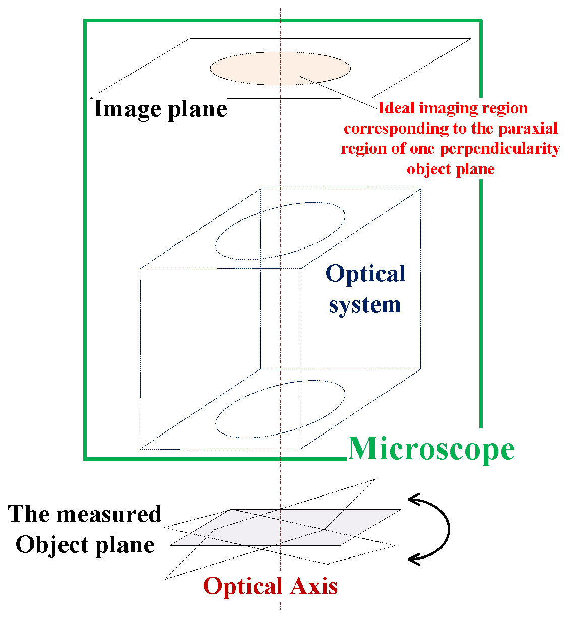
The PSF should be measured on a pre-determined object plane that is perpendicular to the optical axis of the microscopic system (Figure 1). The PSF has a correspondence relationship with an object plane that is perpendicular to the optical axis, and a 3D PSF measurement is used to obtain each PSF on its corresponding perpendicular object plane at the focus depth. Realizing this goal becomes more difficult with super-resolution microscopic measurements. A measured object plane that is not perpendicular to the optical axis results in an obtained PSF that is not homogeneous due to a defocusing effect along with the optical axis direction. Moreover, the accuracy of the PSF is significantly reduced when the PSF does not have a corresponding object plane that is perpendicular to the optical axis. This is especially important when the PSF is employed in 3D super-resolution microscopic image restoration. In this case, all the corresponding object planes within focal depth must be confirmed. Two other microscopic elements are essential when obtaining a PSF: the magnification and the paraxial region. These elements may change with object plane variation along the optical axis. In summary, if the measured object plane that is perpendicular to the optical axis is not determined, the meanings of the PSF, magnification, and paraxial region will be lost for super-resolution microscopic measurements. The common methods for obtaining PSFs stated above are not able to determine the object planes that are perpendicular to the optical axis or the longitudinal height positions of each object plane along the optical axis, as measuring these factors requires more than 3D PSF measurements.
In this paper, a microscope PSF evaluation method for calibrating the object plane that is perpendicular to the optical axis is proposed. The paraxial region, object plane perpendicularity determination, and 3D PSF evaluation methods are presented. The presented methods, together with the integration of dual-spot position detection technology to realize a 3D PSF on the perpendicular object plane, facilitate the magnification and paraxial region evaluation, as well as the confirmation of any microscopic system. The availability of the proposed method is then experimentally verified.
2. Layout of PSF Measurement
The proposed PSF measurement configuration consisted of a movable assembly (PSF calibration module) and a static assembly (light source and Z-axis position measurement charge-coupled devices (CCDs); Figure 2). The core component was a dual position-sensitive-detector (PSD)-based unit [15] that was within the PSF calibration module. The dual PSD-based unit was used to obtain the incident beam direction vector. Here, two PSDs were replaced by two CCDs that could obtain two light spots from two different light routes. In this way, the dual PSD-based unit was able to obtain two incident beam light direction vectors at the same time. When a light beam reached one receiving plane, the intensity distribution of the light spot acted as a form of a Gaussian surface, and the plane position of the light spot was directly obtained by the PSD. The intensity distribution of the light spot was imaged by the CCD, and a Gaussian function was applied to fit the intensity distribution; then, the plane position was obtained by fitting.
The PSF calibration module was integrally fixed on a six-degree-freedom macro/micro displacement platform. The slope face of the rectangular prism containing the polarization refractor plane and polarization splitter plane was parallel to the Y–Z plane of the coordinates, as determined by the dual PSD-based unit. The essential characteristics of the proposed PSF measurement setup included the following (Figure 2):
- A linearly polarized beam of light originated from a fiber-coupled laser (mounted on an adjustor). The linearly polarized beam light could go through the polarization refractor plane and was divided in half by the polarization splitter plane.
- The light beam from the laser was the excitation light of a fluorescent particle. The cover slip acted as an emission filter [16] that only allowed the fluorescent particle’s emission light to travel into the microscope.
- When the linearly polarized light beam reached the Z-position measurement CCD (mounted on an adjustor) from the beam shifting corner cube (CC), after going through the quarter wave plate, it changed into circularly polarized light. A part of this light was reflected by the semi-transparent mirror parallel to the Z-position measurement CCD’s light-sensitive surface. Another part was directed into the Z-position measurement CCD. When the reflected part again went through the quarter wave plate, its linearly polarized direction was perpendicular to the original. This portion was reflected by the polarization refractor plane and directed into the dual PSD-based unit.
3. Core Technologies and Algorithms
3.1. Measurement of the Direction of the Dual PSD-Based Unit’s Incident Beam
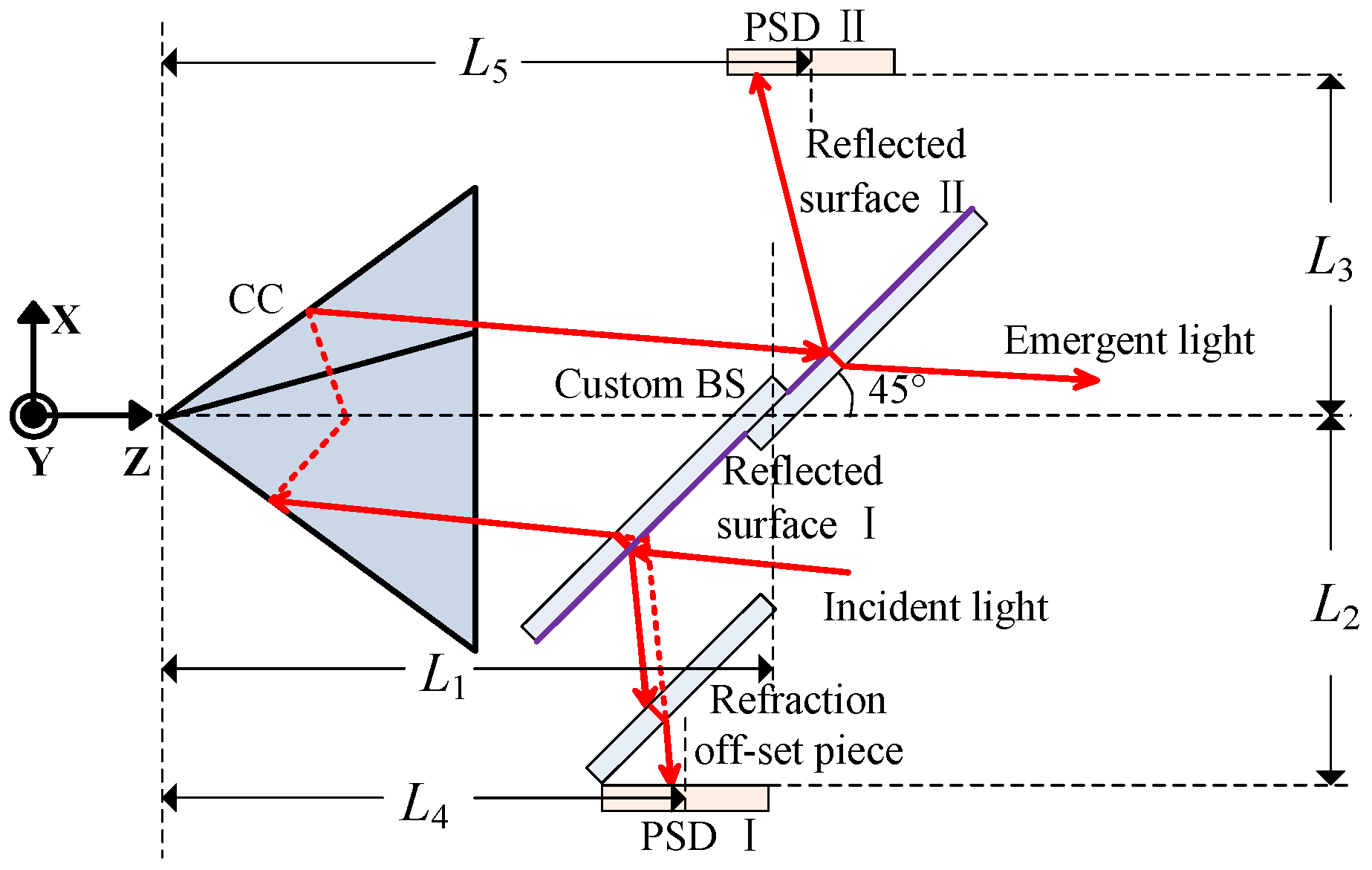
Dual PSD-based units were previously proposed in [15]. In the dual PSD-based unit proposed here, the custom beam splitter (BS) consisted of two BSs, both with coplanar reflecting surfaces. The incident light reflected by the custom BS traversed a refraction offset piece as thick as the first BS and then entered PSD I. The portion of the incident light that was transmitted through the custom BS was partly reflected by a CC and received by PSD II.
In Figure 3, it is seen that the CC joint was located at the origin of the rectangular coordinate system. The cube’s center line (i.e., the Z-axis) and the custom BS’s reflecting surfaces were fixed at an angle of 45°. L1 is the distance between the CC joint and the center point of the custom BS (i.e., the point of intersection between the Z-axis and the custom BS’s reflecting surfaces). L2 and L3 are the distances between the Z-axis and PSD I and PSD II, respectively. L4 and L5 represent the distances between the CC joint and the center points of PSD I and II, respectively. The custom BS’s reflecting surfaces and PSDs were all perpendicular to the X–Z plane, assuming that (y1, z1) and (y2, z2) were the coordinate values of the beam spots on PSD I and II, respectively. It is important to note that (y1, z1) and (y2, z2) are absolute coordinate values, whereas a PSD only measures its own values along its own Y- and Z-axes. Thus, z1 and z2 should actually be z1P + L4 and z2P + L5 in the rectangular coordinate system of Figure 3, respectively, where z1P and z2P are, respectively, the values measured by PSD I and II. In addition, the centers of PSD I and II can deviate from the X–Z plane; here, they are expressed as L6 and L7, respectively. Thus, the values of y1 and y2 should be y1P + L6 and y2P + L7 in the rectangular coordinate system of Figure 3, respectively, where y1P and y2P are the values measured by PSD I and II.
In the rectangular coordinate system of Figure 3, the components of the incident beam unit vector <m, n, q> that arrive at the dual PSD-based unit are:
where 2L1 + L3 − L2 = E, L6 + L7 = Q, 2L1 − L4 − L5 = F, y1P + y2P = M1, z1P + z2P = M2, and . E, Q, and F are parameters of the dual PSD-based unit, and M1 and M2 are the values obtained by PSDs I and II, respectively. The parameters E, Q, and F can be calibrated by the auto-reflection alignment method [17]. In addition, it is clear that the translation motion of the incident beam can be measured by PSD I and II in the dual PSD-based unit.
3.2. Paraxial Region and Object Plane Perpendicularity Determination
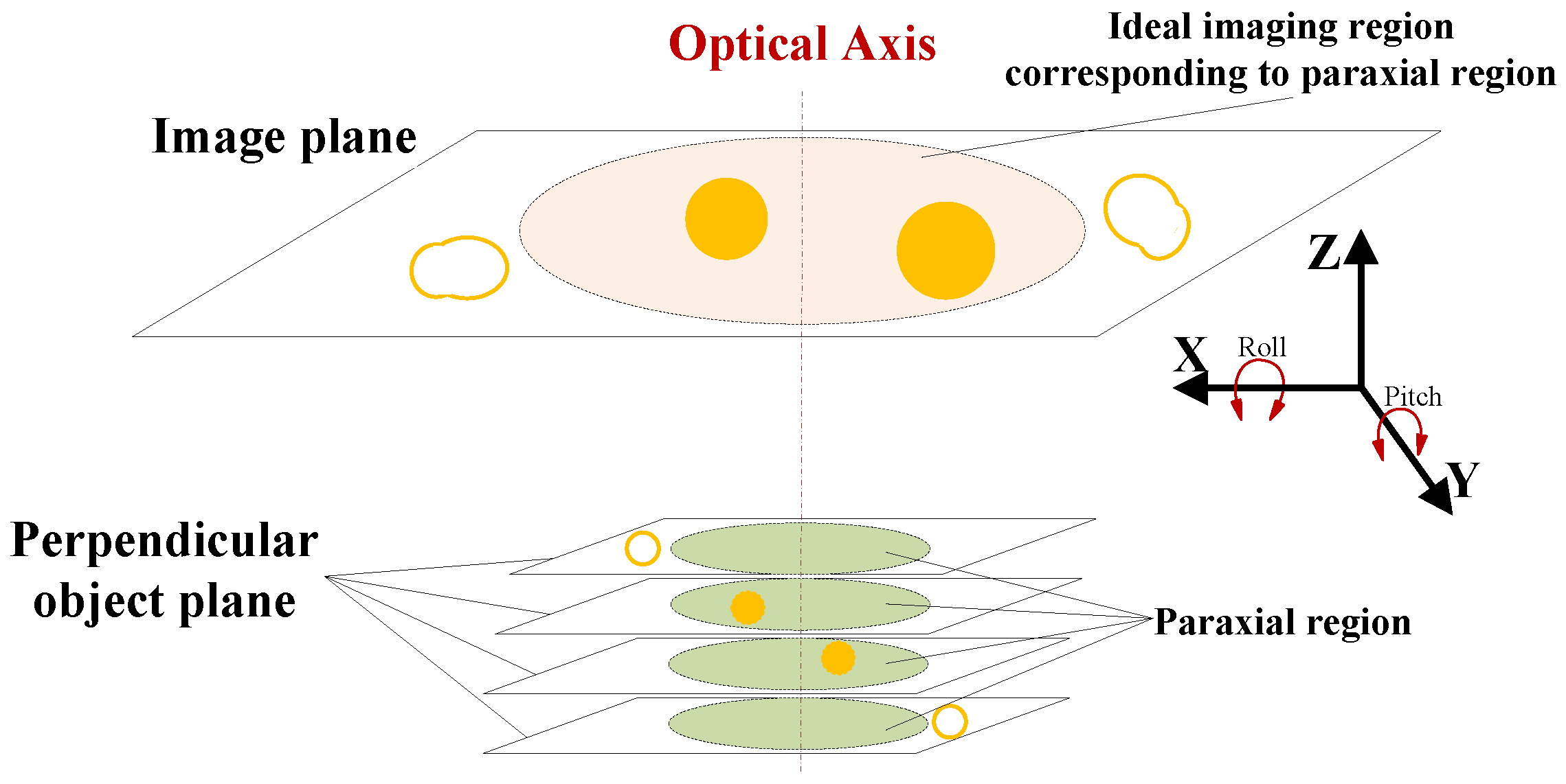
According to the theory of diffraction, there exists a paraxial region of each perpendicular object plane that allows the nanoparticle’s imaging to satisfy an isoplanatic condition (Figure 4). In this paraxial region, the aberrations of the nanoparticle’s imaging can be minimized, and the nanoparticle can be imaged ideally. Moreover, the images of the nanoparticles located in different positions on the paraxial region of some perpendicular object planes are considered to be identical. It is clear that there is one ideal imaging region corresponding to each of the paraxial regions on the imaging plane.
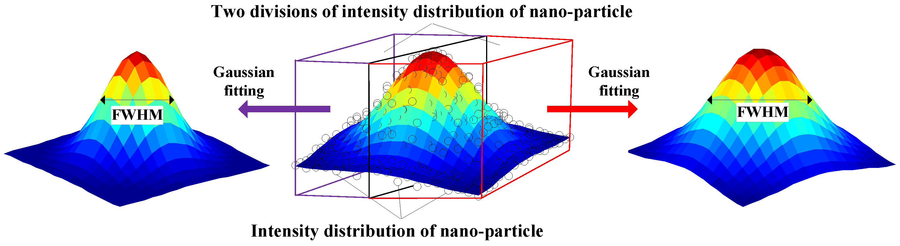
Based on the diffraction imaging analysis, the spot intensity distribution and size of the nanoparticle imaging change with the object plane’s variation. However, the intensity distribution of these spot images is very symmetrical when these images are within the paraxial region of each object plane, and those that are out of the paraxial region are asymmetric due to an aberration in the optical imaging system. In Figure 5, the curve surface was fit with the nanoparticle’s intensity distribution image with a Gaussian function to obtain its central position. Then, we divided the nanoparticle’s intensity distribution longitudinally into two parts by passing through the central position (as shown in Figure 5, where the splitting plane is parallel to the X–Z or Y–Z planes), where the curve surface fit each of the two parts with a Gaussian function. Next, we normalized the two fitting Gaussian surfaces of the two parts of the nanoparticle’s intensity distribution. The full widths at half maximum (FWHM) of the two normalized Gaussian surfaces were obtained, and then the difference between the two FWHMs was also obtained.
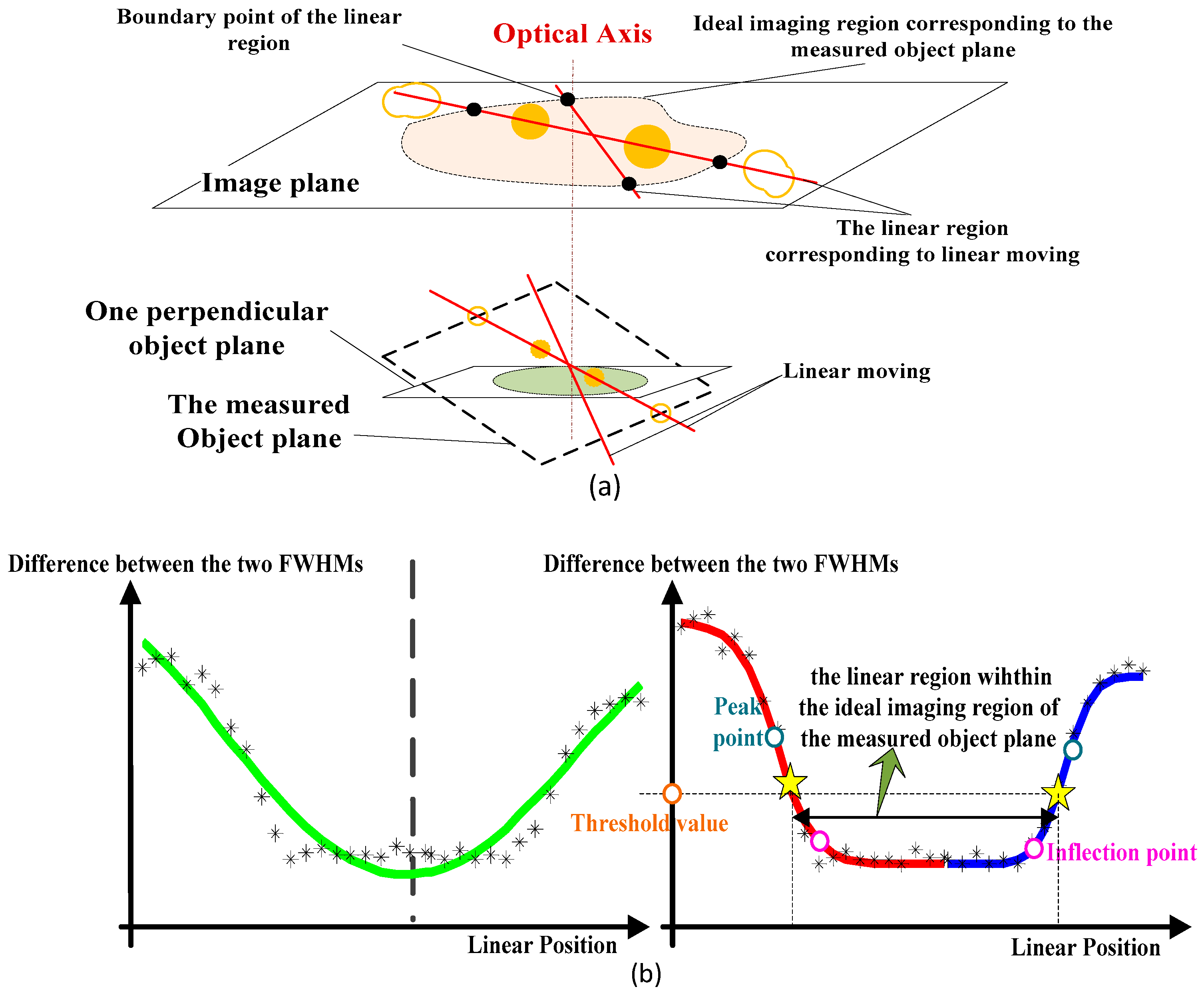
When the measured object plane is non-perpendicular to the optical axis, the images of a nanoparticle that move on this object plane can be considered to be a series of images on different object planes that are perpendicular to the optical axis (Figure 6a). The nanoparticle is moved linearly on the measured object plane to obtain a series of images of the linear position from one border position of the image plane to its opposite border position. For each image, the procedure shown in Figure 5 was run, and a series of differences between the two FWHMs was obtained for each image. Because the images’ intensity distributions within the paraxial region had good symmetry, the differences between two FWHMs within the paraxial region were smaller than those that were not. These differences generally presented a “U” shape, as shown as Figure 6b, where the bottom of the line region is one line in the ideal imaging region of the measured object plane. Notably, the ideal imaging region of the measured object plane (Figure 6a) has some difference from the ideal imaging region of Figure 4 because this series of images was obtained from different perpendicular object planes. In the ideal imaging region of the measured object plane, although isoplanatic conditions could not be met (the sizes of these spot images were not the same), the symmetries of the intensity distribution of these spot images still performed well.
In order to confirm that one object plane is perpendicular to the optical axis, the two boundary points of the linear region must be obtained within the ideal imaging region of the measured object plane. Here, a method of combining quartic polynomial curve fitting with logistic curve fitting was used to confirm the boundary point (Figure 6b). This process is called the polynomial combining logistic curve fitting method and is described as follows.
In Figure 6b, the black star point is a series of the differences between the two FWHMs. Fitting with a quartic polynomial curve to obtain the green line, the second vertex position is split into difference data, where the two divided parts are fitted with logistic curves. The fitting model is:
where K, R, and U are the undetermined coefficients that need to be confirmed through fitting; L is a dependent variable that is, in this case, the difference between the two FWHMs; and s is an independent variable that is, in this case, the linear position when the nanoparticle is moved linearly on the measured object plane. The logistic curve fittings of the front and the rear division parts are represented by the red and blue lines, respectively (Figure 6b). The position values of the red line’s second inflection point and the blue line’s first inflection point are (ln(Rred) – 1.317)/Ured and (ln(Rblue) – 1.317)/Ublue, respectively. The red line’s peak point and the blue line’s peak point are ln(Rred)/Ured and ln(Rblue)/Ublue, respectively. The line segment between the (ln(Rred) – 1.317)/Ured and (ln(Rblue) – 1.317)/Ublue points is chosen. The lowest of the difference values on the (2ln(Rred) – 1.317)/(2Ured) and (2ln(Rblue) – 1.317)/(2Ublue) positions is the threshold value. If the difference values of the positions within the chosen line segment are all below the threshold value, then the chosen line segment is the linear region within the ideal imaging region of the measured object plane, and two boundary points of the chosen line segment are determined. When two of the chosen line segments are obtained, then the four boundary points of the two chosen lines determine the ideal imaging region of the measured object plane (Figure 6a).
To obtain one object plane that is perpendicular to the optical axis and its paraxial region, the following steps should be followed:
- Keep the measured object plane’s space attitude for the pitching and Z-axis position constant. Roll the measured object plane in a small range of –Angle to +Angle.
- After each rolling operation, apply the polynomial combining logistic curve fitting method stated above to determine the ideal imaging region of the measured object plane. In the ideal imaging region, choose the Gaussian function’s FWHM for one spot image as a reference object (here, the spot imaging nearest to the center of the ideal imaging region was chosen). Compare it with the Gaussian function’s FWHM for any other function in the two chosen lines within the ideal imaging region, obtain the difference’s mean square root (RMS) for each compared pair, record the average of these RMS values for the current rolling space attitude, and then choose the measured object plane corresponding to the smallest average of all rolling space attitudes.
- Keep the rolling and Z-axis position of the obtained object plane space attitude constant. Pitch the object plane in a small range and carry out the same operations in steps 1–2. The chosen object plane on this step is one object plane that is perpendicular to the optical axis. Then, again run the polynomial combining logistic curve fitting method on the perpendicular object plane to confirm its ideal imaging region. The paraxial region on some perpendicular object plane has its corresponding ideal imaging region on the image plane (Figure 4). Thus, the confirmation of this ideal imaging region is equal to the confirmation of the paraxial region of the perpendicular object plane.
3.3. D PSF Evaluation
The fluorescent normalization intensity of one fluorescent nanoparticle on the object plane is [18]:
where xo and yo are the coordinate values of the object plane along the X and Y axes, respectively; Dparticle is the diameter of the fluorescent nanoparticle. When only considering geometrical optic imaging, the intensity distribution of the fluorescent nanoparticle image is fparticle (–xi/M, –yi/M) after microscopic magnification, where M is the microscopic magnification and xi and yi are the coordinate values of the imaging plane.
The normalization intensity distribution of the PSF on an object plane can be considered a function of the Gaussian function shape [19,20]:
where is standard deviation ( is the desired value) and the PSF’s FWHM is determined by , FWHMPSF = 2. The normalized microscopic diffraction imaging of one fluorescent nanoparticle is:
where Fimaging (xi, yi) is the normalized intensity distribution of the nanoparticle’s image and the Fimaging (xi, yi) central position can be obtained with the Gaussian function. In this way, it is possible to build the convolution coordinates of Equation (5) to use as the central position for the original point.
In order to obtain I (xi, yi) so that the standard deviation of I (xi, yi) can be obtained, Equation (5) can be used to solve a minimization problem:
Equation (6) can be solved by an iteration algorithm. Choosing a fine initial iteration value plays a very important role in whether or not an ultimate optimum solution is obtained. Due to the FWHM of Fimaging (xi, yi), FWHMimaging is slightly greater than FWHMPSF; particularly, when Dparticle is small, the former is approximately equal to the latter. Therefore, the standard deviation of the initial iteration value can be taken as FWHMimaging/(2).
is the value corresponding to any object plane, and at the focal depth , the variation approximately acts linearly [19]. Here, we used cubic polynomial to fit the variation, where is any position relative to the focal object plane (original position) along the Z-axis; is the value corresponding to the focal object plane; and a, b, and c are fitting coefficients. The 3D PSF can be expressed as:
Obtaining on five perpendicular object planes (the focal object plane and any four perpendicular object planes) can initially provide the coefficients a, b, and c. Therefore, the initial iteration value of Equation (6) can be taken as for the process of obtaining on other perpendicular object planes. All obtained values and their corresponding values are used to determine the new fitting coefficients, a, b, and c. This operation is repeated for the perpendicular object planes as much as possible, ultimately confirming the coefficients a, b, and c.
4. Entire 3D PSF Evaluation Procedure
Regardless of the object plane’s perpendicularity, the ideal imaging region determination of the measured object plane (a polynomial combining the logistic curve fitting method), and the 3D PSF evaluation, it is necessary to measure the PSF calibration module’s spatial orientation and position through the dual PSD-based unit. Combining the statements in Section 3, the total PSF evaluation procedure can be presented as the following steps:
- Place a fluorescent nanoparticle under the microscope for imaging. Adjust the fiber-coupled laser to make its unit direction vector <0, 0, –1> in the coordinates determined by the dual PSD-based unit.
- Determine the object plane’s perpendicularity and the paraxial region, as detailed in Section 3.2. There are a few points to note during this process: i. The PSF calibration module’s spatial orientation (rolling angle α and pitching angle β) and the PSF calibration module’s plane position both need to be confirmed. It is clear that the PSF calibration module’s plane position assurance can be realized by the dual PSD-based unit’s CCD (Figure 2). The PSF calibration module’s spatial orientation can be confirmed by observing the variation of the PSF calibration module’s spatial orientation. The unit direction vector of the light beam from the fiber-coupled laser becomes <mX, nY, qZ >, which is obtained by the dual PSD-based unit. Therefore, according to the transformation of the rectangular coordinates in space, α and β can be solved by the following matrix:ii. After each rolling (or pitching) operation in the procedure of obtaining one object plane that is perpendicular to the optical axis (Section 3.2), the measured object plane is the X–Y plane of the coordinates determined by the dual PSD-based unit, and the unwanted rolling angle and pitching angle caused by movement can also be obtained with Equation (8). The six-degree-freedom macro/micro displacement platform is able to compensate for unwanted spatial orientation according to the rolling and pitching angles that are needed to keep the PSF calibration module’s spatial orientation constant during the process of determining the ideal imaging region of the measured object plane (step 2 in Section 3.2). iii. After each rolling (or pitching) operation, the fiber-coupled laser must be adjusted to make its unit direction vector <0, 0, –1> again and to adjust the Z-position measurement CCD to make the light beam reflected by the semi-transparent mirror normal (namely, to make the unit direction vector of the light beam reflected by the semi-transparent mirror <0, 0, –1> in the coordinates determined by the dual PSD-based unit). Then, the PSF calibration module’s Z-axis direction position in its own coordinates can be confirmed (Z-axis direction position variation can be measured) to make sure the PSF calibration module (fluorescent particle) can stably move on the measured object plane (the X–Y plane of the dual PSD-based unit’s coordinates) and keep its longitudinal space position unchanged.
- After the two steps above, one object plane that is perpendicular to the optical axis is confirmed, and the Z-axis of the dual PSD-based unit’s coordinates becomes the optical axis. The Z-position measurement CCD is adjusted to normally reflect the light beam by the semi-transparent mirror. The light is transmitted through the semi-transparent mirror incidents into the Z-position measurement CCD. Then, the PSF calibration module’s (fluorescent particle’s) Z-axis direction position (longitudinal space position along the optical axis) can be measured by the Z-position measurement’s CCD.
- The polynomial combining logistic curve fitting method is run on different perpendicular object planes along the Z-axis (the optical axis) to determine the paraxial regions. This also determines the magnifications of different perpendicular object planes through the planar translational: magnification = the measured XY displacements on the image plane/the XY displacement measured by the dual PSD-based unit.
- Finally, the 3D PSF evaluation in Section 3.3 is run for perpendicular object planes along the Z-axis to obtain the microscope’s 3D PSF.
5. Experiments and Results
An experiment was used to verify the ability of the proposed method to obtain the 3D PSF. A standard 150 nm diameter fluorescent nanoparticle (Fluorescence Polystyrene, excitation peak: 540 nm; emission peak: 580 nm) was fixed in the cell of the proposed PSF measurement setup (Figure 2). The objective lens’ nominal magnification was 60X (apochromatism objective 0.75 NA) using a commercial microscope, which needed to be calibrated.
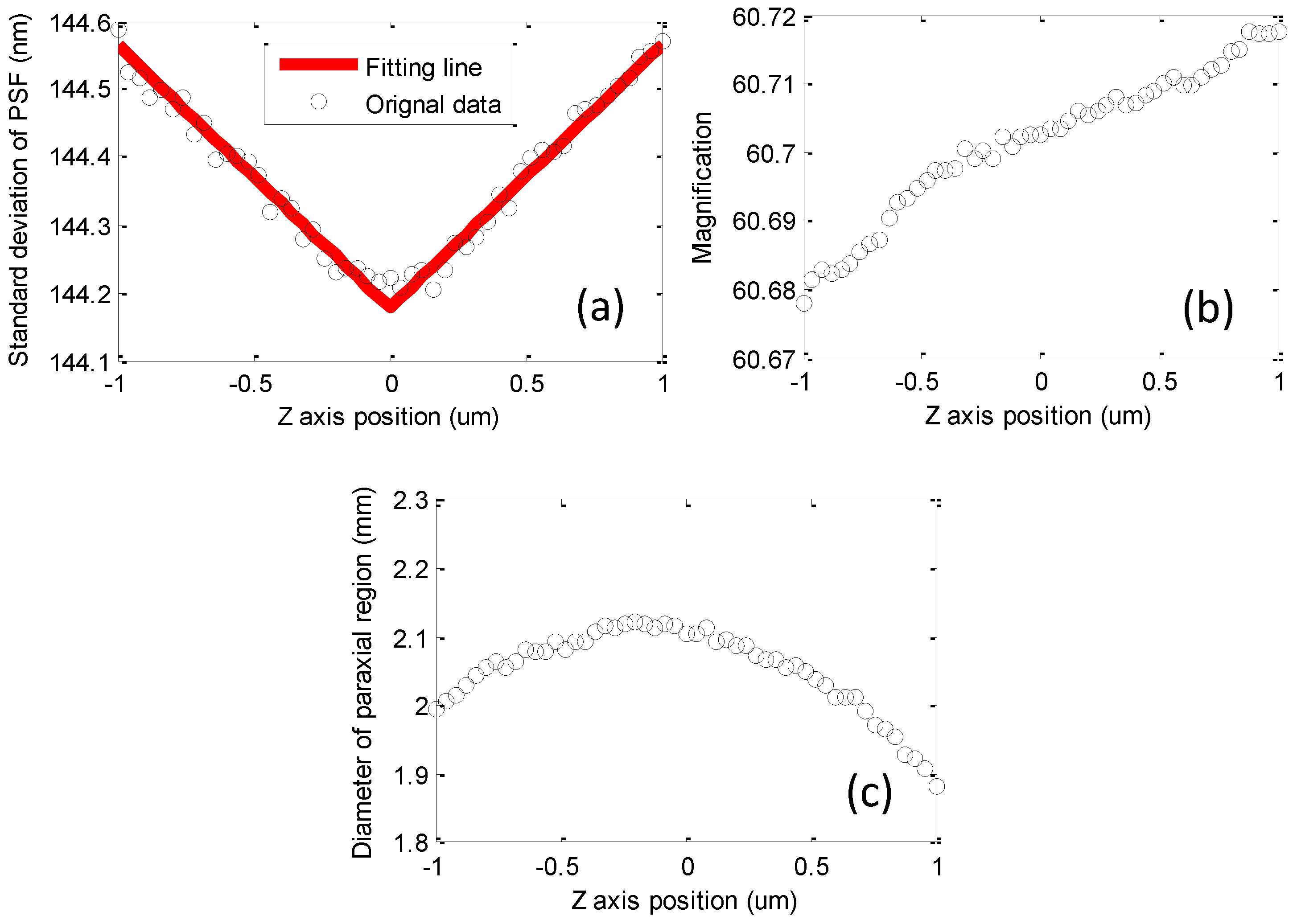
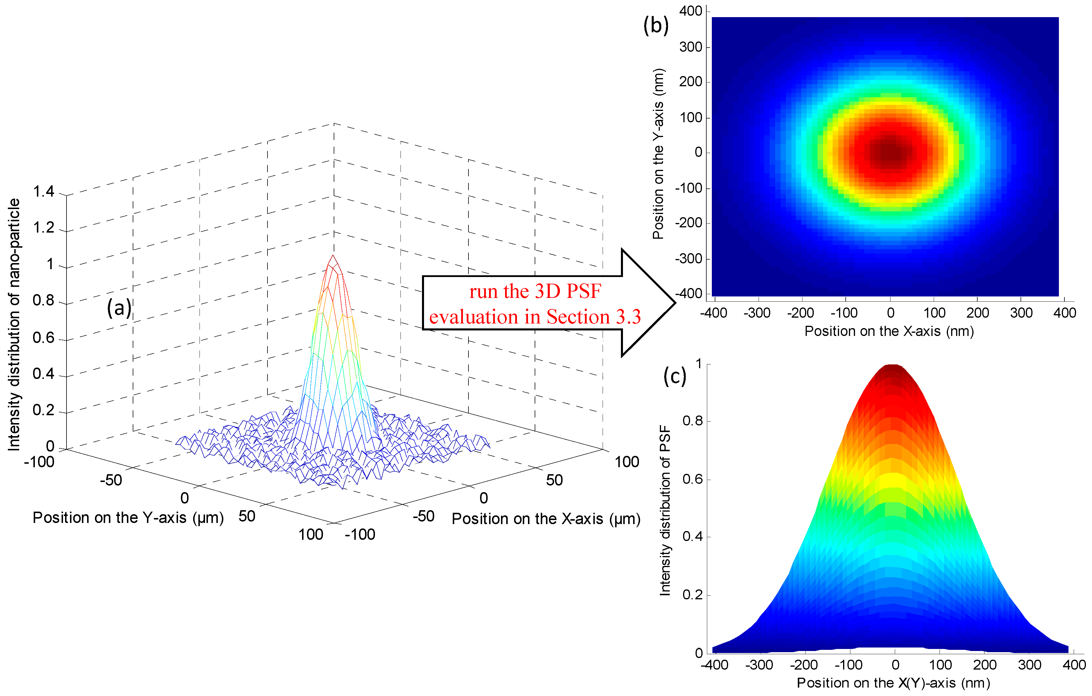
The entire 3D PSF evaluation procedure (Section 4) was run to obtain the results of Figure 7 and Table 1. The focal object plane was used as the original position along the Z-axis, and it was demonstrated that the obtained PSF fitting line closely matched the original data (Figure 7). The cubic polynomial coefficients for fitting the 3D PSF were obtained as detailed in Section 3.3 (Table 1). For the consistency of presentation, here, the mentioned paraxial region was actually its corresponding ideal imaging region on the image plane. The intensity distribution of the nanoparticle’s image and its PSF intensity distribution on the original Z-axis position are shown in Figure 8.
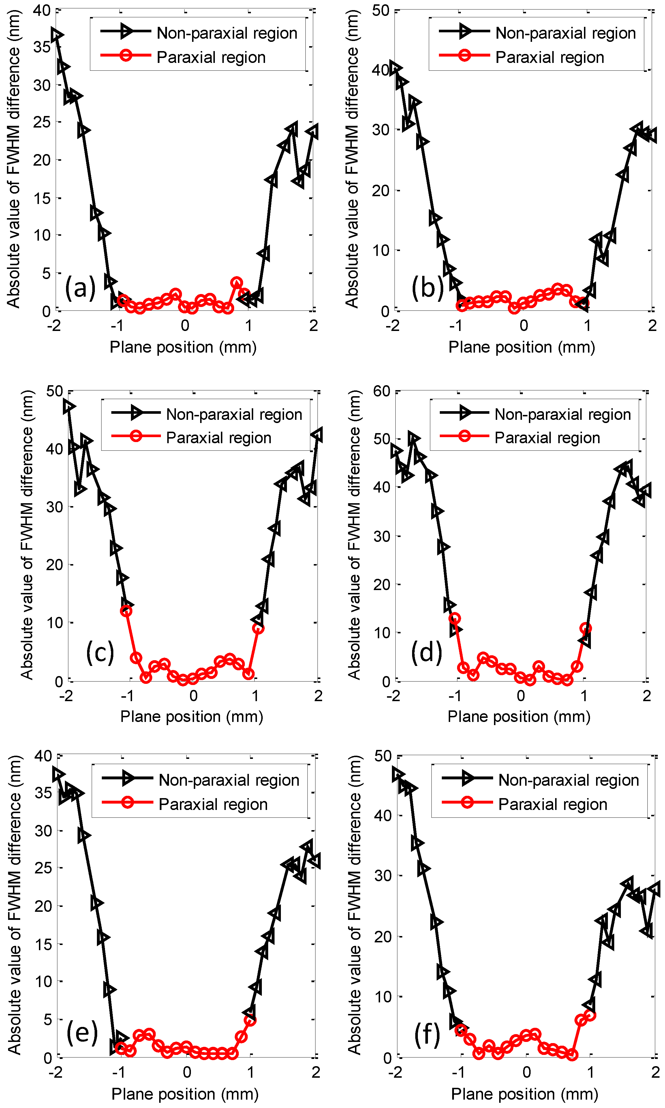
In order to test the results of the 3D PSF evaluation, 100 and 200 nm diameter nanoparticles were measured on the three perpendicular object planes (the Z-axis positions of 0.5, 0, and −0.5 μm) along the Z-axis (the optical axis of the commercial microscope), as well as the three obtained PSFs and magnifications corresponding to the three perpendicular object planes. We compared the FWHMs of the measured and calculated intensity distributions of the 100 and 200 nm diameter nanoparticles (the calculated intensity distributions could be determined by Equation (5)). The FWHM differences between the measured FWHMs and the calculated FWHMs on the three perpendicular object planes demonstrated that the differences clearly defined the paraxial region (Figure 9). The plane position was the distance from the center of the paraxial region. The FWHM differences in the paraxial region (the red line) were almost all below 5 nm (Figure 9). The FWHM differences became bigger with an increase in the deviation from the paraxial region (the black line; Figure 9). This verified that the obtained 3D PSF, magnification, and paraxial region (Figure 7) were correct and also demonstrated the validity of the proposed PSF evaluation method to calibrate the object plane that was perpendicular to the optical axis.
6. Conclusions
In this paper, a point spread function (PSF) evaluation method for a microscope on the object plane that is perpendicular to the optical axis was proposed. This method mainly includes the measurement of a dual PSD-based unit’s incident beam direction, the determination of the paraxial region and the object plane’s perpendicularity, and the evaluation of the 3D PSF. The PSF calibration module involves a dual PSD-based unit that is used to achieve the spatial orientation and position location of the object plane and the fluorescent particle over the entire PSF evaluation process. The proposed method determines the magnification and paraxial region on each perpendicular object plane in the produced 3D PSF evaluation. A standard 150 nm nanoparticle was employed in the proposed PSF evaluation method to obtain the 3D PSF, the magnification, and the paraxial region of the microscope. A comparison of the 100 and 200 nm nanoparticles’ measured FWHMs and calculated FWHMs demonstrated the validity of the proposed PSF evaluation method to obtain the 3D PSF, the magnification, and the paraxial measurements.
Author Contributions
S.M. conceived the experiments, designed the experiments, performed the experiments, analyzed the data, and wrote the paper; Z.W. analyzed the data and designed the experiments; J.P. conceived the experiments. All authors have read and agreed to the published version of the manuscript.
Funding
Research reported in this study is supported by China Postdoctoral Science Foundation (2019M652440), Shandong Provincial Natural Science Foundation, China (Grant No. ZR2018PF014, Grant No. ZR2018MF032, Grant No. ZR2017LF026) and the National Natural Science Foundation of China (Grant No. 61801272).
Conflicts of Interest
The authors declare no conflict of interest.
References
- Robens, C.; Brakhane, S.; Alt, W.; Kleißler, F.; Meschede, D.; Moon, G.; Ramola, G.; Alberti, A. High numerical aperture (NA = 0.92) objective lens for imaging and addressing of cold atoms. Opt. Lett. 2017, 42, 1043–1046. [Google Scholar] [CrossRef] [PubMed] [Green Version]
- Kawata, S.; Arimoto, R.; Nakamura, O. Three-dimensional optical-transfer-function analysis for a laser-scan fluorescence microscope with an extended detector. J. Opt. Soc. Am. A 1991, 8, 171–175. [Google Scholar] [CrossRef]
- Bishara, W.; Su, T.-W.; Coskun, A.F.; Ozcan, A. Lensfree on-chip microscopy over a wide field-of-view using pixel super-resolution. Opt. Express 2010, 18, 11181–11191. [Google Scholar] [CrossRef] [PubMed]
- Nakamura, O.; Kawata, S. Three-dimensional transfer-function analysis of the tomographic capability of a confocal fluorescence microscope. J. Opt. Soc. Am. A 1990, 7, 522–526. [Google Scholar] [CrossRef]
- Rust, M.J.; Bates, M.; Zhuang, X. Sub-diffraction-limit imaging by stochastic optical reconstruction microscopy (STORM). Nat. Methods 2006, 3, 793–795. [Google Scholar] [CrossRef] [PubMed] [Green Version]
- Holden, S.J.; Uphoff, S.; Kapanidis, A.N. DAOSTORM: An algorithm for high—Density super-resolution microscopy. Nat. Methods 2011, 8, 279–280. [Google Scholar] [CrossRef] [PubMed]
- Zhu, L.; Zhang, W.; Elnatan, D.; Huang, B. Faster STORM using compressed sensing. Nat. Methods 2012, 9, 721–723. [Google Scholar] [CrossRef] [PubMed] [Green Version]
- Vermeulen, P.; Zhan, H.; Orieux, F.; Olivo-Marin, J.C.; Lenkei, Z.; Loriette, V.; Fragola, A. Out-of-focus background subtraction for fast structured illumination super-resolution microscopy of optically thick samples. J. Microsc. 2015, 259, 257–268. [Google Scholar] [CrossRef] [PubMed]
- Somekh, M.G.; Hsu, K.; Pitter, M.C. Effect of processing strategies on the stochastic transfer function in structured illumination microscopy. J. Opt. Soc. Am. A 2011, 28, 1925–1934. [Google Scholar] [CrossRef]
- Somekh, M.G.; Hsu, K.; Pitter, M.C. Stochastic transfer function for structured illumination microscopy. J. Opt. Soc. Am A 2009, 26, 1630–1637. [Google Scholar] [CrossRef] [PubMed]
- Somekh, M.G.; Hsu, K.; Pitter, M.C. Resolution in structured illumination microscopy: A probabilistic approach. J. Opt. Soc. Am. A 2008, 25, 1319–1329. [Google Scholar] [CrossRef] [PubMed]
- Haeberlé, O. Focusing of light through a stratified medium: A practical approach for computing microscope point spread functions. Part I: Conventional microscopy. Opt. Commun. 2003, 216, 55–63. [Google Scholar] [CrossRef] [Green Version]
- Rust, M.J.; Mongis, C.; Knop, M. PSFj: Know your fluorescence microscope. Nat. Methods 2014, 11, 981–982. [Google Scholar]
- Hirvonen, L.M.; Wicker, K.; Mandula, O.; Heintzmann, R. Structured illumination microscopy of a living cell. Eur. Biophys. J. 2009, 38, 807–812. [Google Scholar] [CrossRef] [PubMed]
- Hu, P.; Mao, S.; Tan, J.B. Compensation of errors due to incident beam drift in a 3 DOF measurement system for linear guide motion. Opt. Express 2015, 23, 28389–28401. [Google Scholar] [CrossRef] [PubMed]
- Selvaggi, L.; Salemme, M.; Vaccaro, C.; Pesce, G.; Rusciano, G.; Sasso, A.; Campanella, C.; Carotenuto, R. Multiple-Particle-Tracking to investigate viscoelastic properties in living cells. Methods 2010, 51, 20–26. [Google Scholar] [CrossRef] [PubMed]
- Mao, S.; Hu, P.; Ding, X.; Tan, J. Parameter correction method for dual position-sensitive-detector-based unit. Appl. Opt. 2016, 55, 4073–4078. [Google Scholar] [CrossRef] [PubMed]
- Van Der Voort, H.T.M.; Strasters, K.C. Restoration of confocal images for quantitative image analysis. J. Microsc. 1995, 178, 165–181. [Google Scholar] [CrossRef]
- Sarder, P.; Nehorai, A. Deconvolution methods for 3-D fluorescence microscopy images. IEEE Signal Process. Mag. 2006, 23, 32–45. [Google Scholar] [CrossRef]
- Tao, Q.; He, X.; Zhao, J.; Teng, Q.; Chen, J. Image Estimation Based on Depth-Variant Imaging Model in Three-Dimensional Microscopy. In Proceedings of the SPIE—The International Society for Optical Engineering, Beijing, China, 8 February 2005. [Google Scholar]
Figure 1.
The measured object plane is perpendicular to the optical axis of the microscopic system.

Figure 2.
Proposed point spread function (PSF) measurement setup and light routes (red/purple arrows).
Figure 2.
Proposed point spread function (PSF) measurement setup and light routes (red/purple arrows).

Figure 3.
Schematic of the designed dual position-sensitive-detector (PSD)-based unit.

Figure 4.
Imaging of a nanoparticle on different object planes that are perpendicular to the optical axis.
Figure 4.
Imaging of a nanoparticle on different object planes that are perpendicular to the optical axis.

Figure 5.
Fitting the two divisions of the nanoparticle’s intensity distribution with a Gaussian function.
Figure 5.
Fitting the two divisions of the nanoparticle’s intensity distribution with a Gaussian function.

Figure 6.
(a) Imaging of a nanoparticle moving on the measured object plane; (b) polynomial combining the logistic curve fitting method to judge the ideal imaging region of the measured object plane.
Figure 6.
(a) Imaging of a nanoparticle moving on the measured object plane; (b) polynomial combining the logistic curve fitting method to judge the ideal imaging region of the measured object plane.

Figure 7.
The obtained 3D PSF (a), magnification (b), and paraxial region (c).

Figure 8.
Intensity distribution of the nanoparticle’s image (a) and its PSF’s intensity distribution in the X–Y (b) and X–Z (or Y–Z) (c) planes.
Figure 8.
Intensity distribution of the nanoparticle’s image (a) and its PSF’s intensity distribution in the X–Y (b) and X–Z (or Y–Z) (c) planes.

Figure 9.
Full widths at half maximum (FWHM) differences between the measured FWHM and the calculated FWHM for standard 100 nm (a,c,e) and 200 nm (b,d,f) diameter nanoparticles: On the 0.5 μm Z-axis position (a,b); on the original Z-axis position (c,d); and on the −0.5 μm Z-axis position (e,f).
Figure 9.
Full widths at half maximum (FWHM) differences between the measured FWHM and the calculated FWHM for standard 100 nm (a,c,e) and 200 nm (b,d,f) diameter nanoparticles: On the 0.5 μm Z-axis position (a,b); on the original Z-axis position (c,d); and on the −0.5 μm Z-axis position (e,f).


Table 1.
Cubic polynomial coefficients of fitting and .
| a | b | c | ||
|---|---|---|---|---|
| Z-axis positive direction | 8.11 × 10⁻³⁰ | −9.86 × 10⁻³⁰ | −1.11 × 10⁻¹⁶ | 2.08 × 10⁻¹⁴ |
| Z-axis negative direction | 1.14 × 10⁻²⁸ | −1.64 × 10⁻²⁸ | 1.12 × 10⁻¹⁶ | 2.08 × 10⁻¹⁴ |
© 2020 by the authors. Licensee MDPI, Basel, Switzerland. This article is an open access article distributed under the terms and conditions of the Creative Commons Attribution (CC BY) license (http://creativecommons.org/licenses/by/4.0/).
Share and Cite
MDPI and ACS Style
Mao, S.; Wang, Z.; Pan, J. Microscope 3D Point Spread Function Evaluation Method on a Confirmed Object Plane Perpendicular to the Optical Axis. Appl. Sci. 2020, 10, 2430. https://0-doi-org.brum.beds.ac.uk/10.3390/app10072430
AMA Style
Mao S, Wang Z, Pan J. Microscope 3D Point Spread Function Evaluation Method on a Confirmed Object Plane Perpendicular to the Optical Axis. Applied Sciences. 2020; 10(7):2430. https://0-doi-org.brum.beds.ac.uk/10.3390/app10072430
Chicago/Turabian StyleMao, Shuai, Zhenzhou Wang, and Jinfeng Pan. 2020. "Microscope 3D Point Spread Function Evaluation Method on a Confirmed Object Plane Perpendicular to the Optical Axis" Applied Sciences 10, no. 7: 2430. https://0-doi-org.brum.beds.ac.uk/10.3390/app10072430
Note that from the first issue of 2016, this journal uses article numbers instead of page numbers. See further details here.